Abstract

A new approach is proposed, namely CSSF MIMO radar, which applies the technique of step frequency (SF) to compressive sensing (CS) based multi-input multi-output (MIMO) radar. The proposed approach enables high resolution range, angle and Doppler estimation, while transmitting narrowband pulses. The problem of joint angle-Doppler-range estimation is first formulated to fit the CS framework, i.e., as an $\ell_{1}$ optimization problem. Direct solution of this problem entails high complexity as it employs a basis matrix whose construction requires discretization of the angle-Doppler-range space. Since high resolution requires fine space discretization, the complexity of joint range, angle and Doppler estimation can be prohibitively high. For the case of slowly moving targets, a technique is proposed that achieves significant complexity reduction by successively estimating angle-range and Doppler in a decoupled fashion and by employing initial estimates obtained via matched filtering to further reduce the space that needs to be digitized. Numerical results show that the combination of CS and SF results in a MIMO radar system that has superior resolution and requires far less data as compared to a system that uses a matched filter with SF.

Keywords: Compressive sensing, MIMO radar, step frequency, DOA estimation, Doppler estimation, range estimation

I Introduction

Benefiting from the idea of multiple-input multiple-output (MIMO) communication systems, MIMO radar systems have received considerable attention in recent years. A MIMO radar [1]-[3] although having some similarities with phased-array radar, is different in that it transmits multiple waveforms from its antennas, and in general offers a more flexible configuration. A MIMO radar with widely separated antennas [4] views a target from different decorrelated directions and thus enjoys spatial diversity. For MIMO radar with colocated antennas [5][6], independent waveforms enable superior angular resolution as compared to phased-array radar. We focus on the colocated type of MIMO radar throughout this paper.

Compressive sensing (CS) is a relatively recent development [7]-[10] and has already been applied successfully in diverse fields such as image processing and wireless communications. The theory of CS states that a $K$-sparse signal vector $\mathbf{x}$ of length $N$ can be recovered exactly with high probability based on $\mathcal{O}(K\log N)$ measurements via $\ell_{1}$-optimization. Let $\bf\Psi$ denote the basis matrix that spans the space in which the signal is sparse, and $\bf\Phi$ be the measurement matrix that is used to linearly compress the signal. The $\ell_{1}$-optimization problem is formulated as follows:

$$\min\|\mathbf{s}\|_{1},\ \ s.t.\ \text{to}\ {\bf y}=\mathbf{\Phi}{\bf x}=\mathbf{\Phi\Psi}{\bf s}$$ (1)

where $\mathbf{s}$ is an $N\times 1$ sparse vector with $K$ principal elements while the remaining elements can be ignored; $\mathbf{\Phi}$ is an $M\times N$ matrix with $M\ll N$. The product $\mathbf{\Phi\Psi}$ is referred to as the sensing matrix. The uniform uncertainty principle (UUP) [9][11] indicates that if every set of sensing matrix columns with cardinality less than the sparsity of the signal of interest is approximately orthogonal, then the sparse signal can be exactly recovered with high probability. This implies that $\mathbf{\Phi}$ is incoherent with $\mathbf{\Psi}$. Throughput this paper, we will refer to the solution of a problem of the form (1) as the CS approach.

By exploiting the sparsity of radar signals in various spaces, CS has been applied to radar systems [12]-[15] and to MIMO radar [16]-[19]. In [17] and [18], a uniform linear array was considered as a transmit and receive antenna configuration and the CS approach was applied using a submatrix of the identity matrix as the measurement matrix. Bounds on the achievable range and azimuth resolution and the number of recoverable targets were derived in [18]. In [16] and [19], the authors proposed a CS-based MIMO radar system implemented on a small scale network. According to [19], randomly located network nodes, each equipped with a single antenna, serve as transmit and receive antenna elements. The transmit nodes transmit periodic pulses. The receive nodes forward their compressively obtained measurements to a fusion center. Exploiting the sparsity of targets in the angle-Doppler space, an $\ell_{1}$-optimization problem is formulated and solved at the fusion center in order to extract target angle and Doppler information. This approach achieves the superior resolution of MIMO radar with far fewer samples than required by conventional approaches, which implies lower power consumption for the receive nodes.

The application of CS to step-frequency radar (SFR) [24] was investigated in [25]-[27]. SFR transmits pulse trains of varying frequency. Thus, although the individual pulses are relatively long in duration and are narrowband, the transmit signal is effectively wideband. Since range resolution increases with the signal bandwidth, SFR achieves high range resolution. At the same time, SFR does not suffer from low signal-to-noise ratio (SNR) at the receiver typically associated with wideband systems that rely on short duration pulses. In [27], it was found that the CS approach can significantly reduce the number of pulses required by SFR to achieve a certain resolution. A CS-based data acquisition and imaging method was proposed in [25] for stepped-frequency continuous-wave ground penetrating radars, and in [26] CS was applied to stepped-frequency through-the-wall radar imaging. In both cases it was shown that the CS approach can provide a high-quality radar image using many fewer data samples than conventional methods.

In this paper, we consider a more general scenario than that of [16] and [19]. The methods of [16] and [19] assume that the targets are located in a small range bin and the sampling is synchronized with the first target return. Such assumptions do not allow for range estimation. In this paper, the targets can be located across several range bins. We propose CSSF MIMO radar, an approach that applies step frequency to CS-based MIMO radar. Two types of CSSF MIMO radar systems are considered, i.e., linear step-frequency radar (LSFR), and random step-frequency radar (RSFR), and their effects on the CS approach are studied. The proposed approach enables high resolution range as well as angle and Doppler estimation. The problem of joint angle-Doppler-range estimation is first formulated to fit the CS framework, i.e., as an $\ell_{1}$ optimization problem. Solving this problem entails high complexity as it employs a basis matrix whose construction requires discretization of the angle-Doppler-range space. The complexity increases with the size of the basis matrix, or equivalently, as the discretization step decreases; the latter step needs to be as small as possible as it sets the lower limit of resolution. For slowly moving targets, a technique is proposed that successively estimates angle-range and Doppler in a decoupled fashion, and employs initial estimates obtained via a matched filter (MF) to further reduce the space that needs to be digitized. In [20] and [21], information on the support of a sparse signal was used in the minimization process resulting in complexity reduction. In our case, we do not explore the role of initial estimates on the minimization process, as they are not expected to be very reliable. Instead, we use them only as a guide for the construction of the basis matrix. The preliminary results of CSSF MIMO radar and the decoupled scheme were published in [22] and [23] which consider the same signal models as in [16] and [19]. This paper extends the work of [22] and [23] to the general scenario aforementioned and offers an mathematic insight into CSSF MIMO.

The paper is organized as follows. In Section II we provide the signal model of a CS-based MIMO radar system. In Section III, we introduce the proposed CSSF MIMO radar system. A decoupled scheme for CSSF MIMO is described in Section IV. Simulation results are given in Section V for the case of slowly moving targets. Finally, we make some concluding remarks in Section VI.

Notation: Lower case and capital letters in bold denote respectively vectors and matrices. The expectation of a random variable is denoted by $E\{\cdot\}$. Superscripts $(\cdot)^{H}$ and $\mathrm{Tr}(\cdot)$ denote respectively the Hermitian transpose and trace of a matrix. $A(m,n)$ represents the $(m,n)$th entry of the matrix $\bf A$.

II Signal Model for CS-based MIMO Radar

Let us consider the same setting as in [19]. In particular, assume $K$ point targets and colocated transmit (TX)/receive (RX) antennas that are randomly distributed over a small area. The $k$-th target is at azimuth angle $\theta_{k}$ and moves with constant radial speed $v_{k}$. Let $(r^{t}_{i},\alpha^{t}_{i})$/$(r^{r}_{i},\alpha^{r}_{i})$ denote the location of the $i$-th TX/RX node in polar coordinates. The number of TX and RX nodes is denoted by $M_{t}$ and $N_{r}$, respectively. Let $d_{k}(t)$ denote the range of the $k$-th target at time $t$. Under the far-field assumption, i.e., $d_{k}(t)\gg r^{t/r}_{i}$, the distance between the $i$th transmit/receive node and the $k$-th target $d^{t}_{ik}$/$d^{r}_{ik}$ can be approximated as

$$d^{t/r}_{ik}(t)\approx d_{k}(t)-\eta_{i}^{t/r}(\theta_{k})=d_{k}(0)-\eta_{i}^{t/r}(\theta_{k})-v_{k}t$$ (2)

where $\eta_{i}^{t/r}(\theta_{k})=r^{t/r}_{i}\cos(\theta_{k}-\alpha^{t/r}_{i})$.

Assuming that there is no clutter, each TX node transmits periodic pulses of duration $T_{p}$ and pulse repetition interval (PRI) $T$. The target return from the $k$-th target arriving at the $l$-th antenna during the $m$-th pulse is

$$y^{k}_{lm}(t) =\sum_{i=1}^{M_{t}}\beta_{k}x_{i}(t-(d^{t}_{ik}(t)+d^{r}_{lk}(t))/c)\exp({j{2\pi}f(t-(d^{t}_{ik}(t)+d^{r}_{lk}(t))/{c})})$$ (3)

where $c$, $f$ and $\beta_{k}$ denotes the speed of light, the carrier frequency, and the reflection coefficient of the $k$-th target, respectively; $x_{i}(t)$ represents the transmit waveform of the $i$-th node. The demodulated baseband signal corresponding to a single target can be approximated by

$$y^{k}_{lm}(t) \approx\sum_{i=1}^{M_{t}}\beta_{k}x_{i}(t-2d_{k}(0)/c)\exp(-{j{2\pi}f(d^{t}_{ik}(t)+d^{r}_{lk}(t))/{c}}).$$ (4)

In the above equation, the time delays in the received waveforms due to the $k$-th target are all the same and equal to $2d_{k}(0)/c$. This approximation is enabled by the assumption of narrowband transmit waveforms, slowly moving targets and colocated nodes. The fact that the targets can be in different range bins implies that the delays corresponding to different targets will be different. Therefore, sampling the received signal and ensuring that all target returns fall in the sampling window would require time delay estimation. However, in a CS scenario, there are not enough data to obtain such estimates using traditional methods, e.g., the matched filtering method (MFM). In the following, we will extract the range and angle information simultaneously using the CS approach without assuming availability of time delay estimates.

The compressed samples collected by the $l$-th antenna during the $m$-th pulse can be expressed as

$${{\bf r}}_{lm} =\sum_{k=1}^{K}\beta_{k}e^{j2\pi{p}_{lmk}}{\bf\Phi}_{l}{\bf D}(f_{k})\mathbf{C}_{\tau_{k}}{\bf X}{\bf v}(\theta_{k})+{\bf\Phi}_{l}{\bf n}_{lm}$$ (5)

where

1. ${p}_{lmk}=\frac{-2d_{k}(0)f}{c}+\frac{\eta_{l}^{r}(\theta_{k})f}{c}+{f_{k}(m-1)T}$, where $f_{k}=\frac{2v_{k}f}{c}$ is the Doppler shift induced by the $k$-th target; $\mathrm{diag}\{{\bf X}^{H}{\bf X}\}=[1,\ldots,1]^{T}$; $lT_{s},l=0,\ldots,L-1$, represent the time within the pulse (fast time) and thus the pulse duration is $T_{p}=LT_{s}$;

2. $\mathbf{\Phi}_{l}$ is the $M\times(L+\tilde{L})$ measurement matrix for the $l$-th receive node where $\tilde{L}T_{s}$ is the maximum time delay and known in advance. The measurement matrix has elements that are independent and identically distributed (i.i.d) Gaussian random variables;

3. ${\bf v}(\theta_{k})=[e^{j\frac{2\pi f}{c}\eta^{t}_{1}(\theta_{k})},...,e^{j\frac{2\pi f}{c}\eta^{t}_{M_{t}}(\theta_{k})}]^{T}$ and ${\bf D}(f_{k})={\rm diag}\{[e^{j{2\pi}f_{k}0T_{s}},\ldots,e^{j{2\pi}f_{k}(L-1)T_{s}}]\}$;

4. $\tau_{k}=\lfloor\frac{2d_{k}(0)}{cT_{s}}\rfloor$ and ${\bf C}_{\tau_{k}}=[{\bf 0}_{L\times\tau_{k}},{\bf I}_{L},{\bf 0}_{L\times(\tilde{L}-\tau_{k})}]^{T}$. Here, we assume that the target returns completely fall within the sampling window of length $(L+\tilde{L})T_{s}$, and that $T_{s}$ is small enough so that the rounding error in the delay is small, i.e., $x_{i}(t-\tau_{k})\approx x_{i}(t-\lfloor\frac{2d_{k}(0)}{cT_{s}}\rfloor)$.

5. ${\bf n}_{lm}$ is the interference at the $l$-th receiver during the $m$-th pulse, which includes a jammer’s signal and thermal noise.

Let us discretize the angle, speed and range space on a fine grid, i.e., respectively, $[\tilde{a}_{1},\ldots,\tilde{a}_{N_{a}}]$, $[\tilde{b}_{1},\ldots,\tilde{b}_{N_{b}}]$ and $[\tilde{c}_{1},\ldots,\tilde{c}_{N_{c}}]$. Let the grid points be arranged first angle-wise, then range-wise, and finally speed-wise to yield the grid points $(a_{n},b_{n},c_{n}),n=1,...,N_{a}N_{b}N_{c}$. Through this ordering, the grid point $(\tilde{a}_{n_{a}},\tilde{b}_{n_{b}},\tilde{c}_{n_{c}})$ is mapped to point $(a_{n},b_{n},c_{n})$ with $n=(n_{b}-1)n_{a}n_{c}+(n_{c}-1)n_{a}+n_{a}$. We assume that the discretization step is small enough so that each target falls on some angle-speed-range grid point. Then (5) can be rewritten as

$${{\bf r}}_{lm} ={\bf\Phi}_{l}\left(\sum_{n=1}^{N}s_{n}e^{j2\pi{q}_{lmn}}{\bf D}\left(\frac{2b_{n}f}{c}\right)\mathbf{C}_{\lfloor\frac{2c_{n}}{cT_{s}}\rfloor}{\bf X}{\bf v}(a_{n})+{\bf n}_{lm}\right)$$ (6)

where $s_{n}=\left\{\begin{array}[]{ll}\mbox{ reflection coefficient of the target},&\text{if there is a target at}\ (a_{n},b_{n},c_{n})\\ 0,&\text{if there is no target at}\ (a_{n},b_{n},c_{n})\end{array}\right.,$ $N=N_{a}N_{b}N_{c}$, and

$$q_{lmn}=\frac{-2c_{n}f}{c}+\frac{\eta_{l}^{r}(a_{n})f}{c}+\frac{2b_{n}f(m-1)T}{c}.$$ (7)

In matrix form we have

$${{\mathbf{r}}}_{lm}=\mathbf{\Theta}_{lm}{\mathbf{s}}+{\bf\Phi}_{l}{\bf n}_{lm}$$ (8)

where ${\bf s}=[s_{1},...,s_{N}]^{T}$ and

$$\mathbf{\Theta}_{lm}={\bf\Phi}_{l}\underbrace{[e^{j2\pi q_{lm1}}{\bf D}(2b_{1}f/c)\mathbf{C}_{\lfloor\frac{2c_{1}}{cT_{s}}\rfloor}{{\bf X}}{\bf v}(a_{1}),\ldots,e^{j2\pi q_{lmN}}{\bf D}(2b_{N}f/c)\mathbf{C}_{\lfloor\frac{2c_{N}}{cT_{s}}\rfloor}{{\bf X}}{\bf v}(a_{N})]}_{\mathbf{\Psi}_{lm}}.$$ (9)

According to the CS formulation, $\mathbf{\Theta}_{lm}$ is the sensing matrix and $\mathbf{\Psi}_{lm}$ is the basis matrix.

If the number of targets is small as compared to $N$, the positions of the targets are sparse in the angle-speed-range space, i.e., $\mathbf{s}$ is a sparse vector. The locations of the non-zero elements of ${\bf s}$ provide information on target angle, speed and range.

All the receive nodes forward their compressed measurements to a fusion center. We assume that the fusion center has the ability to separate the data of different nodes from each other. This can be done, for instance, if the nodes send their data over different carriers. The fusion center combines the compressively sampled signals due to $N_{p}$ pulses obtained at $N_{r}$ receive nodes to form the vector ${{\bf r}}$. It holds that

$${{\bf r}} \buildrel\triangle\over{=} [{{\bf r}}^{T}_{11},\ldots,{{\bf r}}^{T}_{1N_{p}},\ldots,{{\bf r}}^{T}_{N_{r}N_{p}}]^{T}=\mathbf{\Theta}\mathbf{s}+{\bf n}$$ (10)

where $\mathbf{\Theta}=[(\mathbf{\Theta}_{11})^{T},\ldots,(\mathbf{\Theta}_{1N_{p}})^{T},\ldots,(\mathbf{\Theta}_{N_{r}N_{p}})^{T}]^{T}$ and ${\bf n}=[({\bf\Phi}_{1}{\bf n}_{11})^{T},\ldots,({\bf\Phi}_{1}{\bf n}_{1N_{p}})^{T},\ldots,({\bf\Phi}_{N_{r}}{\bf n}_{N_{r}N_{p}})^{T}]^{T}$.

Subsequently, using the predefined measurement matrices, ${\mathbf{\Phi}}_{l},\ l=1,...,N_{r}$, based on the discretization of the angle-speed-range space, and also based on knowledge of the waveform matrix ${\bf X}$, the fusion center recovers $\mathbf{s}$ by applying the Dantzig selector [28] to (10) as

$$\hat{{\bf s}}=\min\|{\bf s}\|_{1}\ \ \ s.t.\ \|{\mathbf{\Theta}}^{H}({\bf r}-\mathbf{\Theta}{\bf s})\|_{\infty}<\mu.$$ (11)

According to [28], the sparse vector ${\bf s}$ can be recovered with very high probability if $\mu=(1+t^{-1})\sqrt{2\log N\tilde{\sigma}^{2}}\sigma_{max}$, where $t$ is a positive scalar, $\sigma_{max}$ is the maximum norm of columns in the sensing matrix $\Theta$, and $\tilde{\sigma^{2}}$ is the variance of the interference in (10). A numerical method to determine the value of $\mu$ is described in [28].

III Introducing Step Frequency to CS-MIMO radar

Let us consider a MIMO radar system in which the carrier frequency of the $m$-th pulse equals

$$f_{m}=f+\Delta f_{m}$$ (12)

where $f$ is the center carrier frequency and $\Delta f_{m}$ denotes the frequency step, $m=1,\ldots,N_{p}$.

The baseband samples collected by the $l$-th antenna during the $m$-th pulse can be expressed as

$$\tilde{{\bf r}}_{lm} ={\bf\Phi}_{l}\sum_{k=1}^{K}\beta_{k}e^{j2\pi\tilde{p}_{lmk}}{\bf D}(f_{mk})\mathbf{C}_{\tau_{k}}{\bf X}{\bf v}_{m}(\theta_{k})+{\bf\Phi}_{l}{\bf n}_{lm}$$ (13)

where

$$\ f_{mk} =\frac{2v_{k}f_{m}}{c},{\bf v}_{m}(\theta_{k})=[e^{j\frac{2\pi f_{m}}{c}\eta^{t}_{1}(\theta_{k})},...,e^{j\frac{2\pi f_{m}}{c}\eta^{t}_{M_{t}}(\theta_{k})}]^{T}$$

$$\mathrm{and}\ \tilde{p}_{lmk} =\frac{-2d_{k}(0)f_{m}}{c}+\frac{\eta_{l}^{r}(\theta_{k})f_{m}}{c}+{f_{mk}(m-1)T}.$$ (14)

Then, based on discrete grid points of the angle-speed-range space, (13) can be rewritten as

$$\tilde{{\bf r}}_{lm} = {\bf\Phi}_{l}\tilde{{\bf\Psi}}_{lm}{\bf s}+{\bf\Phi}_{l}{\bf n}_{lm}$$ (15)

$$= \tilde{\mathbf{\Theta}}_{lm}{\bf s}+{\bf\Phi}_{l}{\bf n}_{lm}$$

where

$$\tilde{\mathbf{\Psi}}_{lm} =[e^{j2\pi\tilde{q}_{lm1}}{\bf D}(2b_{1}f_{m}/c)\mathbf{C}_{\lfloor\frac{2c_{1}}{cT_{s}}\rfloor}{{\bf X}}{\bf v}_{m}(a_{1}),\ldots,e^{j2\pi\tilde{q}_{lmN}}{\bf D}(2b_{N}f_{m}/c)\mathbf{C}_{\lfloor\frac{2c_{N}}{cT_{s}}\rfloor}{{\bf X}}{\bf v}_{m}(a_{N})],$$

$$\tilde{q}_{lmn} =\frac{-2c_{n}f_{m}}{c}+\frac{\eta_{l}^{r}(a_{n})f_{m}}{c}+\frac{2b_{n}f_{m}(m-1)T}{c},$$

$$\mathrm{and}\ \tilde{{\bf\Theta}}_{lm} ={\bf\Phi}_{l}\tilde{{\bf\Psi}}_{lm}.$$ (16)

At the fusion center, the compressively sampled signals due to $N_{p}$ pulses obtained at $N_{r}$ receive nodes are stacked as

$$\tilde{{\bf r}} \buildrel\triangle\over{=}\tilde{\mathbf{\Theta}}\mathbf{s}+{\bf n}$$ (17)

where

$$\tilde{\mathbf{\Theta}}=[(\tilde{\mathbf{\Theta}}_{11})^{T},\ldots,(\tilde{\mathbf{\Theta}}_{1N_{p}})^{T},\ldots,(\tilde{\mathbf{\Theta}}_{N_{r}N_{p}})^{T}]^{T}.$$ (18)

Recovery of $\mathbf{s}$ is performed as in (11) where $\mathbf{\Theta}$ is replaced with $\tilde{\mathbf{\Theta}}$.

In the remainder of the paper, we make the two assumptions:

• (A1) The targets are slowly moving. Therefore, the Doppler shift within a pulse can be ignored, i.e., $f_{m}(2T_{s}(L+\tilde{L}-1)b_{n})/c\approx 0,\ n=1,\ldots,N$.

• (A2) The radar waveforms are independent across transmit nodes and thus $\int_{t=0}^{T}x_{i}(t)x^{*}_{i^{\prime}}(t+\tau)dt,i\neq i^{\prime}$ is negligible as compared to $\int_{t=0}^{T}x_{i}(t)x^{*}_{i}(t+\tau)dt$.

III-A Range resolution

In this subsection we study the relationship between range resolution and the ambiguity function. For the conventional radar systems that uses a matched filter to extract target information, the ambiguity function (AF) characterizes the response to a point target and determines resolution. Let us assume that there is a target at $(\theta,d,v)$. The matched filter looking for a target at $(\theta^{\prime},d^{\prime},v^{\prime})$ yields

$$\chi(\Delta d,\Delta v,\theta,\theta^{\prime})=\sum_{l=1}^{N_{r}}\sum_{i,i^{\prime}=1}^{M_{t}}\sum_{m=1}^{N_{p}}\chi_{i,i^{\prime},m}(\Delta d,\Delta v)e^{j2\pi f_{m}\frac{\eta_{i}^{t}(\theta)+\eta_{l}^{r}(\theta)-\eta_{i^{\prime}}^{t}(\theta^{\prime})-\eta_{l}^{r}(\theta^{\prime})-2\Delta d}{c}}$$ (19)

where $\Delta d=d-d^{\prime}$, $\Delta v=v-v^{\prime}$ and

$$\chi_{i,i^{\prime},m}(\Delta d,\Delta v)\triangleq\int_{t}x_{i}(t)x^{*}_{i^{\prime}}(t+2\Delta d/c)e^{j2\pi f_{m}\frac{2\Delta v}{c}t}dt.$$ (20)

Equation (19) is the AF for SF MIMO radar, where SF MIMO radar refers to MIMO radar that uses the SF technique. Unlike the AF for MIMO radar [29], the carrier frequency is varying between pulses in (19).

To investigate the range resolution let us set $\Delta v=0$ and $\theta=\theta^{\prime}$. Then, the AF becomes

$$\chi(\Delta d,0,\theta,\theta) =N_{r}\sum_{i,i^{\prime}=1}^{M_{t}}\sum_{m=1}^{N_{p}}\chi_{i,i^{\prime},m}(\Delta d,0)e^{j2\pi f_{m}\frac{\eta_{i}^{t}(\theta)-\eta_{i^{\prime}}^{t}(\theta)-2\Delta d}{c}}$$

$$=N_{r}\underbrace{\sum_{m=1}^{N_{p}}e^{j2\pi f_{m}(-2\Delta d/c)}}_{\chi_{1}(\Delta d)}\underbrace{\sum_{i=i^{\prime}}\int_{t}x_{i}(t)x^{*}_{i^{\prime}}(t+2\Delta d/c)}_{\chi_{2}(\Delta d)}dt+N_{r}\underbrace{\sum_{m=1}^{N_{p}}\sum_{i\neq i^{\prime}}e^{j2\pi f_{m}\frac{\eta_{i}^{t}(\theta)-\eta_{i^{\prime}}^{t}(\theta)-2\Delta d}{c}}\int_{t}x_{i}(t)x^{*}_{i^{\prime}}(t+2\Delta d/c)}_{\Delta\chi(\Delta d)}dt$$

Due to (A2), the term $\Delta\chi(\Delta d)$ is negligible as compared to the product $\chi_{1}(\Delta d)\chi_{2}(\Delta d)$ in (III-A). One can see that $\chi_{1}(\Delta d)$ and $\chi_{2}(\Delta d)$ are respectively the AF of SF single-input single-output (SISO) radar and MIMO radar, both for $\Delta v=0$ and $\theta=\theta^{\prime}$. It can seen from (III-A) that a colocated MIMO radar has no gain on range resolution as compared to a SISO radar, i.e., the range resolution of MFSF MIMO radar is at least equal to the best between the range resolution of SF SISO radar and SISO radar, where MFSF MIMO radar refers to matched filter based MIMO radar that uses the SF technique.

In [30], in a study of CS-based SISO radar, it was observed that the maximum value of the correlation of two different columns of the basis matrix is equal to the second largest value of the discrete AF surface. The recovery performance of CS approaches, however, is directly related to the column correlation of the sensing matrix rather than the basis matrix. Unlike [30], we next study the relation of the AF and the column correlation of the sensing matrix for the proposed CSSF MIMO radar. This analysis will provide a clue for comparing the resolution of CS and matched filter in the context of SF MIMO radar, i.e., CSSF MIMO radar and MFSF MIMO radar.

On letting ${\bf p}_{k}$ denote the column of the sensing matrix $\tilde{\mathbf{\Theta}}$ corresponding to the $k$-th grid point in the angle-speed-range space, we have

$$<{\bf p}_{k},{\bf p}_{k^{\prime}}> =\sum_{l=1}^{N_{r}}\sum_{m=1}^{N_{p}}e^{j2\pi(\tilde{q}_{lmk}-\tilde{q}_{lmk^{\prime}})}{\bf v}_{m}^{H}(a_{k^{\prime}}){\bf X}^{H}{\bf C}_{\lfloor\frac{2c_{k^{\prime}}}{cT_{s}}\rfloor}^{H}{\bf D}^{H}\left(\frac{2b_{k^{\prime}}f_{m}}{c}\right)\underbrace{{\mathbf{\Phi}}_{l}^{H}{\mathbf{\Phi}}_{l}}_{{\bf A}}\underbrace{{\bf D}\left(\frac{2b_{k}f_{m}}{c}\right){\bf C}_{\lfloor\frac{2c_{k}}{cT_{s}}\rfloor}{\bf X}{\bf v}_{m}(a_{k})}_{\mathbf{g}_{k}}$$

$$=\sum_{l=1}^{N_{r}}\sum_{m=1}^{N_{p}}\sum_{p,q=1}^{L+\tilde{L}}e^{j2\pi(\tilde{q}_{lmk}-\tilde{q}_{lmk^{\prime}})}{g}^{*}_{k^{\prime}}(p){g}_{k}(q){A}(p,q)$$

$$=\sum_{l=1}^{N_{r}}\sum_{m=1}^{N_{p}}\sum_{p,q=1}^{L+\tilde{L}}\sum_{i,i^{\prime}=1}^{M_{t}}{A}(p,q)e^{j2\pi f_{m}(\eta_{i}^{t}(a_{k})+\eta_{l}^{r}(a_{k})-\eta_{i^{\prime}}^{t}(a_{k^{\prime}})-\eta_{l}^{r}(a_{k^{\prime}})-2\Delta d_{kk^{\prime}}+2\Delta v_{kk^{\prime}}(m-1)T+2T_{s}(b_{k}(q-1)-b_{k^{\prime}}(p-1)))/c}$$

$$\cdot x_{i}\left((q-1)T_{s}-\frac{2c_{k}}{c}\right)x^{*}_{i^{\prime}}\left((p-1)T_{s}-\frac{2c_{k^{\prime}}}{c}\right)$$ (22)

where $\Delta d_{kk^{\prime}}=c_{k}-c_{k^{\prime}}$ and $\Delta v_{kk^{\prime}}=b_{k}-b_{k^{\prime}}$. For simplicity, in the above we assumed that the receive nodes use the same measurement matrix; thus the index $l$ was dropped in ${\bf A}$.

Taking the elements of the measurement matrix ${\bf\Phi}$ to be independent and Gaussian $\mathcal{N}(0,\frac{1}{L+\tilde{L}})$, the expectation of $<{\bf p}_{k},{\bf p}_{k^{\prime}}>$ with respect to the elements of ${\bf\Phi}$ equals

$$E\{<{\bf p}_{k},{\bf p}_{k^{\prime}}>\} =\frac{M}{L+\tilde{L}}\sum_{l=1}^{N_{r}}\sum_{m=1}^{N_{p}}\sum_{i,i^{\prime}=1}^{M_{t}}e^{j2\pi f_{m}(\eta_{i}^{t}(a_{k})+\eta_{l}^{r}(a_{k})-\eta_{i^{\prime}}^{t}(a_{k^{\prime}})-\eta_{l}^{r}(a_{k^{\prime}})-2\Delta d_{kk^{\prime}}+2\Delta v_{kk^{\prime}}(m-1)T)/c}$$

$$\cdot\sum_{p=1}^{L+\tilde{L}}x_{i}\left((p-1)T_{s}-\frac{2c_{k}}{c}\right)x^{*}_{i^{\prime}}\left((p-1)T_{s}-\frac{2c_{k^{\prime}}}{c}\right)e^{j2\pi f_{m}(2T_{s}(p-1)\Delta v_{kk^{\prime}})/c}$$

$$\propto\chi(\Delta d_{kk^{\prime}},\Delta v_{kk^{\prime}},a_{k},a_{k^{\prime}}).$$ (23)

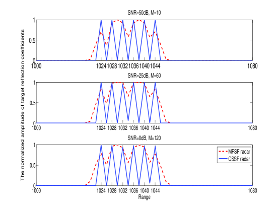
Figure 2: Normalized amplitude estimates of target reflection coefficients for the CSSF radar and MFSF radar (one realization for $M_{t}=N_{r}=1$ and $N_{p}=30$).

One can see from the above equation that the expectation of the column correlation of the sensing matrix is proportional to the discrete AF. To focus on the range resolution we set $a_{k}=a_{k^{\prime}}$ and $\Delta v_{kk^{\prime}}=0$. Essentially, the range resolution of MFSF MIMO radar corresponds to the smallest range difference between two targets, $\Delta d_{kk^{\prime}}$, that sets the AF to zero. Based on the UUP in [11], however, the coherence of the sensing matrix does not have to be zero for exact recovery; a small level of coherence is good enough. Therefore, CS-based radar systems have the potential to improve range resolution. This possibility will be confirmed via simulations in Section V (see Fig. 2).

III-B The effect of signal bandwidth on CSSF-MIMO radar

In an LSFR system, the carrier frequency increases by a constant step between pulses, i.e., $\Delta f_{m}=(m-1)\Delta f$. This type of SF radar can be efficiently implemented using the Inverse Discrete Fourier Transform (IDFT) [24]; however, it suffers from range ambiguity if the distance between a target and receive nodes exceeds the value $R_{u}=\frac{cT}{2}$. The range ambiguity can be removed by randomly choosing the step frequency within a fixed bandwidth at the expense of increased sidelobe as compared to the LSFR [32]. In this section, we investigate the effect of the number of pulses $N_{p}$ (or equivalently, the bandwidth) on range resolution for two types of CSSF MIMO radar, i.e., LSFR and RSFR, in terms of the coherence of the sensing matrix (see (31)). Consistent with [32], which discussed convectional radar systems using the MFM, we find that the RSFR requires more pulses than LSFR to achieve the same range resolution for CS-based MIMO radar.

Since an increase in the number of receive nodes does not improve the range resolution, for simplicity we consider one receive node only. The correlation of columns ${\bf p}_{k}$ and ${\bf p}_{k^{\prime}}$ for $a_{k}=a_{k^{\prime}}$ and $b_{k}=b_{k^{\prime}}$ equals

$$p_{kk^{\prime}} =|<{\bf p}_{k},{\bf p}_{k^{\prime}}>|=\left|\sum_{m=1}^{N_{p}}\sum_{p,q=1}^{L+\tilde{L}}e^{j2\pi f_{m}(-2\Delta d_{kk^{\prime}})/c}{g}^{*}_{k^{\prime}}(p){g}_{k}(q){A}(p,q)\right|$$

$$=\left|\sum_{m=1}^{N_{p}}e^{j2\pi f_{m}(-2\Delta d_{kk^{\prime}})/c}\sum_{p,q=1}^{L+\tilde{L}}{A}(p,q)e^{j2\pi f_{m}(2T_{s}b_{k}(q-p))/c}\left(\sum_{i=1}^{M_{t}}Q_{kk^{\prime}}(m,p,q,i,i)+\sum_{i\neq i^{\prime}}^{M_{t}}Q_{kk^{\prime}}(m,p,q,i,i^{\prime})\right)\right|$$ (24)

where

$$Q_{kk^{\prime}}(m,p,q,i,i^{\prime})=e^{j2\pi f_{m}(\eta_{i}^{t}(a_{k})-\eta_{i^{\prime}}^{t}(a_{k}))/c}x_{i}\left((q-1)T_{s}-\frac{2c_{k}}{c}\right)x^{*}_{i^{\prime}}\left((p-1)T_{s}-\frac{2c_{k^{\prime}}}{c}\right).$$ (25)

Due to (A1) and the discretized version of (A2), we can ignore the Doppler shift within a pulse and the second term $\sum_{i\neq i^{\prime}}^{M_{t}}Q_{kk^{\prime}}(m,p,q,i,i^{\prime})$ in (III-B). Therefore, (III-B) becomes

$$p_{kk^{\prime}} \approx\left|\sum_{m=1}^{N_{p}}e^{j2\pi f_{m}(-2\Delta d_{kk^{\prime}})/c}\sum_{p,q=1}^{L+\tilde{L}}{A}(p,q)\sum_{i=1}^{M_{t}}x_{i}\left((q-1)T_{s}-\frac{2c_{k}}{c}\right)x^{*}_{i}\left((p-1)T_{s}-\frac{2c_{k^{\prime}}}{c}\right)\right|.$$ (26)

Eq. (26) can be rewritten as

$$p_{kk^{\prime}}\approx\left\{\begin{array}[]{ll}{N_{p}}\rho_{kk}&k=k^{\prime}\\ \underbrace{\left|\sum_{m=1}^{N_{p}}e^{j\alpha_{kk^{\prime}}(f+\Delta f_{m})}\right|}_{h(\mathbf{\Delta f})}\rho_{kk^{\prime}}&k\neq k^{\prime}\end{array}\right.\$$ (29)

where $\mathbf{\Delta}f=[\Delta f_{1},\ldots,\Delta f_{N_{p}}]$,

$$\rho_{kk^{\prime}} =\left|\sum_{p,q=1}^{L+\tilde{L}}\sum_{i=1}^{M_{t}}{A}(p,q)x_{i}((q-1)T_{s}-\frac{2c_{k}}{c})x^{*}_{i}((p-1)T_{s}-\frac{2c_{k^{\prime}}}{c})\right|$$

$$\mathrm{and}\ \alpha_{kk^{\prime}} =-\frac{4\pi\Delta d_{kk^{\prime}}}{c}.$$ (30)

Then, the coherence of the sensing matrix $\tilde{\bf\Theta}$ corresponding to columns ${\bf p}_{k}$ and ${\bf p}_{k^{\prime}}$ can be written as

$$\mu_{kk^{\prime}}(\tilde{\bf\Theta})=\frac{p_{kk^{\prime}}}{\sqrt{p_{kk}p_{k^{\prime}k^{\prime}}}}\approx\frac{h(\mathbf{\Delta f})\rho_{kk^{\prime}}}{N_{p}\sqrt{\rho_{kk}\rho_{k^{\prime}k^{\prime}}}}.$$ (31)

III-B1 Linear step frequency

If the carrier frequency increases by a constant step $\Delta f$ between adjacent pulses, i.e., $\Delta f_{m}=(m-1)\Delta f$, then

$$\mu_{kk^{\prime}}(\tilde{\bf\Theta}) \approx\frac{|1-e^{j\alpha_{kk^{\prime}}\Delta fN_{p}}|\rho_{kk^{\prime}}}{|1-e^{j\alpha_{kk^{\prime}}\Delta f}|N_{p}\sqrt{\rho_{kk}\rho_{k^{\prime}k^{\prime}}}}\propto\frac{|\sin(\frac{1}{2}\alpha_{kk^{\prime}}\Delta fN_{p})|}{N_{p}}.$$ (32)

It can be easily seen that an increase in $N_{p}$ tends to reduce the coherence and thus improves the range resolution.

Let $\alpha_{kk^{\prime}ii^{\prime}}^{pq}$ denote the travel-time difference between the signals sent from the transmit node $i$ to the target located at the $k$th grid point at time instant $pT_{s}$, and from the transmit node $i^{\prime}$ to the target located at the $k^{\prime}$th grid point at time instant $qT_{s}$. It holds that

$$\alpha_{kk^{\prime}ii^{\prime}}^{pq}=(-2\Delta d_{kk^{\prime}}+2T_{s}b_{k}(q-p)+\eta_{i}^{t}(a_{k})-\eta_{i^{\prime}}^{t}(a_{k}))/c.$$ (33)

Regarding the approximation error, the term discarded in (26) is

$$\tilde{p}_{kk^{\prime}} =\sum_{m=1}^{N_{p}}e^{j2\pi f_{m}(-2\Delta d_{kk^{\prime}})/c}\sum_{p,q=1}^{L+\tilde{L}}{A}(p,q)e^{j2\pi f_{m}(2T_{s}b_{k}(q-p))/c}\sum_{i\neq i^{\prime}}^{M_{t}}Q_{kk^{\prime}}(m,p,q,i,i^{\prime})$$

$$=\sum_{p,q=1}^{L+\tilde{L}}\frac{1-e^{j2\pi N_{p}\Delta f\alpha_{kk^{\prime}ii^{\prime}}^{pq}}}{1-e^{j2\pi\Delta f\alpha_{kk^{\prime}ii^{\prime}}^{pq}}}e^{j2\pi f\alpha_{kk^{\prime}ii^{\prime}}^{pq}}{A}(p,q)\sum_{i\neq i^{\prime}}^{M_{t}}x_{i}\left((q-1)T_{s}-\frac{2c_{k}}{c}\right)x^{*}_{i^{\prime}}\left((p-1)T_{s}-\frac{2c_{k^{\prime}}}{c}\right).$$ (34)

The amplitude of $\frac{1-e^{j2\pi N_{p}\Delta f\alpha_{kk^{\prime}ii^{\prime}}^{pq}}}{1-e^{j2\pi\Delta f\alpha_{kk^{\prime}ii^{\prime}}^{pq}}}e^{j2\pi f\alpha_{kk^{\prime}ii^{\prime}}^{pq}}$ is bounded by $N_{p}$. For independent waveforms, the approximation error $\tilde{p}_{kk^{\prime}}$ in (III-B) is always negligible as compared to ${p}_{kk^{\prime}}$.

Let $\mu_{t}$ denote the maximum coherence of $\tilde{\bf\Theta}$ that guarantees exact recovery of the sparse vector with high probability via the Dantzig selector. The minimum number of pulses required to achieve a certain resolution can be obtained by solving

$$N_{p}^{*} =\min\ N_{p}$$

$$s.t.\ \frac{|1-e^{j\alpha_{kk^{\prime}}\Delta fN_{p}}|\rho_{kk^{\prime}}}{|1-e^{j\alpha_{kk^{\prime}}\Delta f}|N_{p}\sqrt{\rho_{kk}\rho_{k^{\prime}k^{\prime}}}}\leq\mu_{t},$$

$$k,k^{\prime}=1,\ldots,N\ \mathrm{and}\ k\neq k^{\prime}.$$ (35)

The above problem is easy to solve, for example by trying different values for $N_{p}$; however, it requires a value for $\mu_{t}$. In [18], a rough estimate of $\mu_{t}$ in the presence of mild interference was offered. In general, $\mu_{t}$ must be determined experimentally.

III-B2 Random step frequency

Assuming that the frequency steps over pulses are i.i.d uniform random variables, i.e., $\Delta f_{m}\sim U(0,2b)$, the expectation of square coherence over $\Delta f_{m}$ is given by

$$E\{\mu^{2}_{kk^{\prime}}(\tilde{\bf\Theta})\} =E\left\{\frac{\left|\sum_{m=1}^{N_{p}}e^{j\alpha_{kk^{\prime}}(f+\Delta f_{m})}\rho_{kk^{\prime}}\right|^{2}}{N_{p}^{2}{\rho_{kk}\rho_{k^{\prime}k^{\prime}}}}\right\}$$

$$=\frac{\rho_{kk^{\prime}}^{2}}{{\rho_{kk}\rho_{k^{\prime}k^{\prime}}}}\left(\frac{1}{N_{p}}+\frac{N^{2}_{p}-N_{p}}{N^{2}_{p}}\frac{\sin^{2}(\alpha_{kk^{\prime}}b)}{\alpha_{kk^{\prime}}^{2}b^{2}}\right).$$ (36)

For a fair comparison, we set LSFR and RSFR to cover the same frequency band, i.e., set $b$ equal to $\Delta f(N_{p}-1)/2$. Then (III-B2) can be rewritten as

$$E\{\mu^{2}_{kk^{\prime}}(\tilde{\bf\Theta})\} =\frac{\rho^{2}_{kk^{\prime}}}{{\rho_{kk}\rho_{k^{\prime}k^{\prime}}}N_{p}}\left(1+\frac{4\sin^{2}(\frac{1}{2}(N_{p}-1)\alpha_{kk^{\prime}}\Delta f)}{(N_{p}-1)\alpha_{kk^{\prime}}^{2}\Delta f^{2}}\right)$$ (37)

$$=\frac{\rho^{2}_{kk^{\prime}}}{{\rho_{kk}\rho_{k^{\prime}k^{\prime}}}N_{p}}\left(1+\frac{\sin^{2}(\frac{1}{2}(N_{p}-1)\alpha_{kk^{\prime}}\Delta f)}{(N_{p}-1)(2\pi\Delta f\Delta d_{kk^{\prime}}/c)^{2}}\right).$$

As the term $(2\pi\Delta f\Delta d_{kk^{\prime}}/c)^{2}$ increases, the expected value of the squared coherence becomes approximately equal to $1/N_{p}$. This holds when the product of radian frequency step $2\pi\Delta f$ and the range spacing of grid points $\Delta d_{kk^{\prime}}$ is comparable to the speed of light $c$.

Since the coherence of the sensing matrix for RSFR cannot be obtained directly, we instead compare the squared coherence of the sensing matrix for LSFR and RSFR. For large $N_{p}$, we find from (32) and (37) that the squared coherence for LSFR and RSFR decreases inverse proportionally to $N^{2}_{p}$ and $N_{p}$, respectively. This implies that more pulses are required by RSFR to achieve the desired performance with all other parameters, i.e., $M_{t}$, $N_{r}$ and $M$, being equal.

Before ending this section, we note that the expectation of the approximation error in (III-B) can be represented by

$$\tilde{p}_{kk^{\prime}} =\sum_{p,q=1}^{L+\tilde{L}}e^{j2\pi\alpha^{pq}_{kk^{\prime}ii^{\prime}}(N_{p}-1)\Delta f/2+f}\frac{N_{p}}{N_{p}-1}\frac{2\sin(\pi\alpha^{pq}_{kk^{\prime}ii^{\prime}}(N_{p}-1)\Delta f)}{{\alpha^{pq}_{kk^{\prime}ii^{\prime}}2\pi\Delta f}\bf}A(p,q)\sum_{i\neq i^{\prime}}^{M_{t}}x_{i}\left((q-1)T_{s}-\frac{2c_{k}}{c}\right)x^{*}_{i^{\prime}}\left((p-1)T_{s}-\frac{2c_{k^{\prime}}}{c}\right)$$ (38)

where one can see that a decrease in the product of $\alpha^{pq}_{kk^{\prime}ii^{\prime}}$ (seen in (33)) and the radian frequency step, $2\pi\Delta f$, increases both the approximation error and the squared coherence. Given $\alpha^{pq}_{kk^{\prime}ii^{\prime}}$, an increase in $\Delta f$ would reduce the approximation error $\tilde{p}_{kk^{\prime}}$. However, this would increase the bandwidth required by RSFR.

IV Decoupled estimation of angle, velocity and range with reduced complexity

Solving the $\ell_{1}$ minimization problem of (11) requires polynomial time in the dimension of $\mathbf{s}$. For the discretization discussed in Section II, the joint estimation of angle, velocity and range requires complexity of $\mathcal{O}((N_{a}N_{b}N_{c})^{3})$ [31][28]. For large values of $N_{a}$, $N_{b}$ and $N_{c}$, the computational cost of the CS approach would be prohibitive. In the following, we propose a decoupled angle-velocity-range estimation approach which reduces the search space and thus the computational complexity.

The scheme needs some initial rough estimates of angle and range. One way to obtain those estimates is to use the MFM, which requires forwarding to the fusion center Nyquist sampled data from one pulse. In the following, all $N_{r}$ nodes in the system sample all received pulses in a compressive fashion, except $\tilde{N_{r}}$ nodes, which sample the first received pulse at the Nyquist rate and all remaining pulses in a compressive fashion. Those Nyquist rate samples will be used to obtain coarse estimates of angle and range via the MFM.

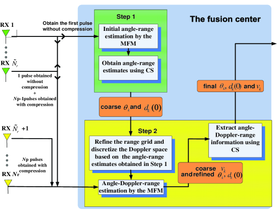
Figure 1: Schematic diagram of the proposed decoupled scheme.

The fusion center performs the following operations (also see Fig. 1).

1. STEP1: Angle and range estimation

   This step uses the first pulse forwarded by each receive node. A fine grid, $(a_{n_{1}},c_{n_{1}}),\ldots,(a_{n_{K_{1}}},c_{n_{K_{1}}})$, is constructed around the MFM initial estimates. Then the sensing matrix is constructed as

   $$\tilde{\mathbf{\Theta}}_{1}={\bf\Phi}_{l1}[e^{j2\pi f_{1}(-2c_{n_{1}}+\eta_{l}^{r}(a_{n_{1}}))/c}\mathbf{C}_{\lfloor\frac{2c_{n_{1}}}{cT_{s}}\rfloor}{{\bf X}}{\bf v}_{m}(a_{n_{1}}),\ldots,e^{j2\pi f_{1}(-2c_{n_{K_{1}}}+\eta_{l}^{r}(a_{n_{K_{1}}}))/c}\mathbf{C}_{\lfloor\frac{2c_{n_{K_{1}}}}{cT_{s}}\rfloor}{{\bf X}}{\bf v}_{m}(a_{n_{K_{1}}})]$$ (39)

   where

   $${{\bf\Phi}}_{lm}=\left\{\begin{array}[]{rl}{\bf I}_{L+\tilde{L}},&l=1,\ldots,\tilde{N_{r}},\ m=1\\ \mathrm{the\ measurement\ matrix\ of\ size}\ M\times({L+\tilde{L}}),&\mathrm{otherwise}\end{array}\right.\ .$$ (42)

   The received signals, $\tilde{\mathbf{r}}_{11},\ldots,\tilde{\mathbf{r}}_{N_{r}1}$, are stacked in a vector, i.e.,

   $$\tilde{{\bf r}}_{1}=\tilde{\mathbf{\Theta}}_{1}{\bf s}+{\bf n}_{1}$$ (43)

   where $\tilde{{\bf r}}_{1}=[\tilde{\mathbf{r}}_{11}^{T},\ldots,\tilde{\mathbf{r}}^{T}_{N_{r}1}]^{T}$. By applying the Dantzig selector to (43), new and refined angle-range information is obtained.

   Thanks to the initial estimates, the search area in the angle-range plane is significantly reduced and thus the computational load of CS is lightened. Due to the fact that only one pulse from each receive node is used, the range resolution at this step is limited by $\frac{c}{2B}$, where $B$ is the signal bandwidth. The obtained range estimates will be refined in the next step in which the fusion center will jointly process the entire pulse train. Also, due to assumption (A1), Doppler information cannot be extracted at this step.

2. STEP 2: Range resolution improvement and Doppler estimation

   In this step the fusion center processes the entire pulse train forwarded by each receive node. The range space around the range estimates obtained in Step 1 is discretized into finer grid points. Based on a discretization of the Doppler space, the refined range grid points and the angle estimates obtained in Step 1, i.e., $(a_{m_{1}},b_{m_{1}},c_{m_{1}}),\ldots,(a_{m_{K_{2}}},b_{m_{K_{2}}},c_{m_{K_{2}}})$, the fusion center formulates a sensing matrix and extracts angle-Doppler-range information in a CS fashion.

   To further reduce the complexity of CS reconstruction, the MFM can be applied before CS to provide angle-Doppler-range estimates around which a finer grid can be constructed and used by CS. In that case MFM would be applied based on the grid points $(a_{m_{1}},b_{m_{1}},c_{m_{1}}),\ldots,(a_{m_{K_{2}}},b_{m_{K_{2}}},c_{m_{K_{2}}})$.

   For the case in which there are stationary targets and moving targets, the angle estimation can be further improved by taking into account Doppler information.

Assuming that the MFM is used for initial estimation, the complexity of two steps is respectively $\mathcal{O}(N_{a}N_{c}(\tilde{N}_{r}L+(N_{r}-\tilde{N}_{r})M)+K_{1}^{3})$ and $\mathcal{O}(K_{2}(\tilde{N}_{r}(L-M)+N_{r}N_{p}M)+K_{3}^{3})$, where $K_{3}$ is the number grid points used by CS at Step 2. Generally, it holds that $K_{1}^{3}+K_{3}^{3}\ll N_{a}N_{c}(\tilde{N}_{r}L+(N_{r}-\tilde{N}_{r})M)+K_{2}(\tilde{N}_{r}(L-M)+N_{r}N_{p}M)$ for a small number of targets. Therefore, the computational load is mostly due to the initial estimation. As compared to the complexity of the joint angle-Doppler-range CS approach, i.e., $\mathcal{O}((N_{a}N_{b}N_{c})^{3}$, considerable computations can be saved by using the proposed decoupled scheme for large values of $N_{a},N_{b}$ and $N_{c}$.

The computation savings, however, may be obtained at the expense of detection accuracy, unless the initial estimates provided by the initial estimation method are reliable. Reliable estimates here refer to the initial estimates whose distances to the true target locations are within the resolution cell that is determined by the initial estimation. Then all the targets can be captured based on the finer angle-range grid points constructed around the reliable initial estimates. For the instance of the MFM, the performance in providing good initial estimates depends on several factors; (i) the signal-to-interference ratio (SIR), which can be improved by employing more data; (ii) angular, range or Doppler resolution, which is improved by increasing $N_{r}$ or $N_{p}$; (iii) the distance between the adjacent grid points. (In the worst case in which the targets fall midway between grid points, the targets may fail to be captured by the closest grid points if the spacing of adjacent grid points is too large. An empirical approach to select grid spacing was discussed in [19]. That approach is also applicable to the MFM); and (iv) the threshold for hard detection. A small threshold should be used in order to reduce the miss probability. However, this implies that more grid points need to be considered for the CS approach following the MFM as compared to a larger threshold. In summary, the performance of the MFM can be improved at the expense of more transmit power and increased complexity.

V Simulation Results

We consider a MIMO radar system with transmit and receive nodes uniformly distributed on a disk of radius $10$m. The carrier frequency is $f=5GHz$. Each transmit node uses orthogonal Hadamard waveforms of length $L=512$ and unit power. The received signal is corrupted by zero-mean Gaussian noise. The signal-to-noise ratio (SNR) is defined as the inverse of the power of thermal noise at a receive node. A jammer is located at angle $7\textordmasculine$ and transmits an unknown Gaussian random waveform. The targets are assumed to fall on the grid points. Throughout this section, the CS approach uses a measurement matrix with Gaussian entries.

V-A Range resolution of the CS-based SFR and conventional SFR

In this subsection we provide some simulation results to show the superiority of CSSF MIMO radar as compared to MFSF MIMO radar in terms of range resolution. Figure 2 shows the normalized amplitude estimates of target reflection coefficients for CSSF MIMO radar and MFSF MIMO radar in one realization. Since the multiple colocated antennas fail to improve range resolution, we consider a single transmit and receive antenna here for simplicity. Let $M=10$, $N_{p}=30$ and the carrier frequencies be randomly selected within the frequency band $[5,5.029]GHz$. The CSSF radar uses $10$ measurements per pulse while MFSF radar obtains $665$ measurements per pulse. Various values of SNR are considered. The spacing between two adjacent grid points is $2m$. There are six targets at ranges $[1024,\ 1028,\ 1032,\ 1036,\ 1040,\ 1044]$m. Figure 2 shows that the peaks corresponding to all targets can be distinguished from each other for the CSSF radar while for the MFSF radar some peaks are lost. This verifies the observations of Section III-A that CSSF radar has the potential to achieve higher range resolution than does MFSF radar.

V-B Range estimation for CSSF MIMO radar

The goal of this subsection is to test the performance of CSSF MIMO radar based on LSF and RSF. Figure 3 compares the numerical and theoretical squared coherence of the sensing matrix corresponding to two adjacent grid points in the range plane for different numbers of pulses and various values of the linear frequency step $\Delta f=1MHz$, $4MHz$ and $8MHz$. All the results shown in Fig. 3 are the numerical squared coherence averaged over 100 independent and random runs and the theoretical squared coherence for LSFR and RSFR calculated based on (32) and (III-B2). We consider the case in which $M_{t}=M=10$, $N_{r}=1$ and the grid step is $\Delta c=7.5m$. For a fair comparison, we choose random step frequencies within the same frequency band as in LSFR, i.e., $f+[0,(N_{p}-1)\Delta f]$. It can be easily seen that the numerical squared coherence of the sensing matrix for LSFR perfectly matches with the theoretical results in (32). The numerical squared coherence of the sensing matrix for RSFR approaches the theoretical results in (III-B2) as $\Delta f$ increases and approaches $1/N_{p}$ as the number of pulses increases. It is also verified by Fig. 3 that LSFR exhibits lower coherence of the sensing matrix than does RSFR.

Figure 4 shows the receiver operating characteristic (ROC) curves of the range estimates produced by the random and linear step-frequency technique based on 200 random and independent runs. Here, the probability of detection (PD) is the percentage of cases in which all the targets are detected. The probability of false alarm (PFA) is the percentage of cases in which false targets are detected. We consider a case in which the angle and speed of three targets are the same and assumed to be known. In each independent run, the target angle and speed are randomly generated. The ranges of three targets are fixed to $1005m$, $1010m$ and $1045m$, respectively. The power of the jammer signal is $4$ and SNR$=0$dB. We can see that the use of LSF yields better performance than randomly choosing the carrier frequency within the same frequency band. In this particular case, CS-based RSFR requires 12 pulses to generate the ROC performance that can be achieved by CS-based LSFR using only $9$ pulses. The performance of LSFR and RSFR based on the MFM is also shown in Fig. 4. It can be seen that the former using $12$ pulses is far better than the latter with the same number of pulses. It can also be seen that CSSF MIMO radar outperforms MFSF MIMO radar.

V-C The joint angle-Doppler-range estimation of CSSF MIMO radar

Figure 5 shows the ROC curves of the angle-speed-range estimates yielded by CSSF MIMO radar using the decoupled scheme. The angle-speed-range estimates have been obtained based on $200$ random and independent runs. The cases in which $M_{t}=10$, $N_{r}=\tilde{N_{r}}=7$ and $N_{p}=12$ are shown in Fig. 5. The azimuth angle and range of three targets are randomly generated in each run but the spacing of angle and range between targets are fixed to $0.3\textordmasculine$ and $7.5m$, respectively. The speeds of three targets are $10m/s,30m/s,$ and $60m/s$. The power of the jammer signal is $4$ and SNR$=0$dB. The performance of MFSF MIMO radar, shown in Fig. 5, is obtained in the same decoupled fashion, i.e., 1) estimate target angle and range based on a single pulse; then refine the angle estimates based on the finer angle grid points around the initial angle estimates by using the MFM; and then 2) process the entire pulse train to extract angle-speed-range information by discretizing the speed space, constructing finer range grid points around the initial range estimates and utilizing the initial angle estimates obtained in 1). One can see that MFSF MIMO radar is inferior to CSSF MIMO radar even when using far more measurements than the latter.

VI Conclusions

We have presented a CSSF MIMO radar system that applies SF to CS-based MIMO radar. The technique of SF can significantly improve range resolution. We have shown that CSSF MIMO radar has the potential to achieve better resolution than MFSF MIMO radar, and that more pulses are required by RSFR than by LSFR to achieve the desired performance with all other parameters being the same. The angle-Doppler-range estimation requires discretization of the angle-Doppler-range space into a large number of grid points, which would increase the complexity of the CS approach. We have presented a CSSF MIMO radar scheme that by decoupling angle-range estimation and Doppler estimation achieves significant complexity reduction. The proposed technique applies to slowly moving targets and relies on initial rough angle-range estimates. Assuming that the initial estimates do not miss any targets, the proposed low complexity scheme maintains the high resolution of the CS approach.

Acknowledgment

The authors would like to thank Dr. Rabinder Madan of the Office of Naval Research for sharing his ideas on the use of compressive sampling in the context of MIMO radar.

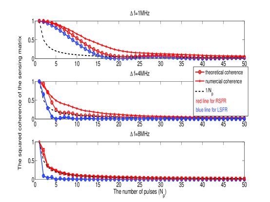
Figure 3: Average squared coherence of the sensing matrix for different numbers of pulses $N_{p}$ over $100$ independent and random runs ($\Delta f=4\times 10^{6}$, $M=M_{t}=10$ and $N_{r}=1$). The distance of two grid points in the range plane is $\Delta c=7.5m$.

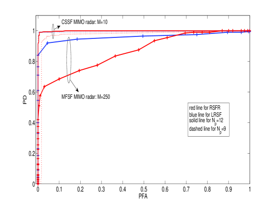
Figure 4: ROC of range estimates obtained with linearly and randomly stepped frequency CSSF MIMO radar and MFSF MIMO radar ($M=M_{t}=10$, $N_{r}=1$ and $\Delta f=1MHz$).

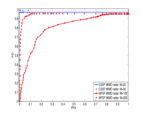
Figure 5: ROC of target detection based on angle-speed-range estimates yielded by the proposed decoupled scheme in Section IV for CSSF MIMO radar and MFSF MIMO radar ($M_{t}=10,N_{r}=\tilde{N_{r}}=7$ and $N_{p}=12$).

References

- [1] E. Fishler, A. Haimovich, R. Blum, D. Chizhik, L. Cimini and R. Valenzuela, “MIMO radar: An idea whose time has come,” in Proc. IEEE Radar Conf., Philadelphia, PA, pp. 71-78, Apr. 2004.
- [2] L. Xu, J. Li and P. Stoica, “Radar imaging via adaptive MIMO techniques,” in Proc. European Signal Process. Conf., Florence, Italy, Sep. 2006.
- [3] J. Li, P. Stoica, L. Xu and W. Roberts, “On parameter identifiability of MIMO radar,” IEEE Signal Process. Lett., vol. 14, no. 12, pp. 968-971, Dec. 2007.
- [4] A.M. Haimovich, R.S. Blum and L.J. Cimini, “MIMO radar with widely separated antennas,” IEEE Signal Process. Magazine, vol. 25, no. 1, pp. 116-129, Jan. 2008.
- [5] P. Stoica and J. Li, “MIMO radar with colocated antennas,” IEEE Signal Processing Magazine, vol. 24, no. 5, pp. 106-114, Sep. 2007.
- [6] C. Chen and P.P. Vaidyanathan, “MIMO radar space-time adaptive processing using prolate spheroidal wave functions,” IEEE Trans. Signal Process., vol. 56, no. 2, pp. 623-635, Feb. 2008.
- [7] D.V. Donoho, “Compressed sensing,” IEEE Trans. Information Theory, vol. 52, no. 4, pp. 1289-1306, Apr. 2006.
- [8] E.J. Candes, “Compressive sampling,” in Proc. The International Congress of Mathematicians, Madrid, Spain, pp. 1433-1452, Aug. 2006.
- [9] E.J. Candes and M.B. Wakin, “An introduction to compressive sampling [A sensing/sampling paradigm that goes against the common knowledge in data acquisition],” IEEE Signal Process. Magazine, vol. 25, no. 2, pp. 21-30, Mar. 2008.
- [10] J. Romberg, “Imaging via compressive sampling [Introduction to compressive sampling and recovery via convex programming],” IEEE Signal Process. Mag., vol. 25, no. 2, pp. 14-20, Mar. 2008.
- [11] E.J. Candes, J.K. Romberg and T. Tao, “Stable signal recovery from incomplete and inaccurate measurements,” Communications on Pure and Applied Mathematics, vol. 59, no. 8, pp. 1207-1223, Aug. 2006.
- [12] R. Baraniuk and P. Steeghs, “Compressive radar imaging,” in Proc. IEEE Radar Conference, Boston, MA, pp. 128-133, Apr. 2007.
- [13] A.C. Gurbuz, J.H. McClellan and W.R. Scott, “Compressive sensing for GPR imaging,” in Proc. 41th Asilomar Conf. Signals, Syst. Comput, Pacific Grove, CA, pp. 2223-2227, Nov. 2007.
- [14] M.A. Herman and T. Strohmer, “High-resolution radar via compressed sensing,” IEEE Trans. Signal Process., vol. 57, no. 6, pp. 2275-2284, Jun. 2009.
- [15] M. Herman and T. Strohmer, “Compressed sensing radar,” in Proc. IEEE Int’l Conf. Acoust. Speech Signal Process., Las Vegas, NV, pp. 2617-2620, Mar.-Apr. 2008.
- [16] A.P. Petropulu, Y. Yu and H.V. Poor, “Distributed MIMO radar using compressive sampling,” in Proc. 42nd Asilomar Conf. Signals, Syst. Comput., Pacific Grove, CA, pp. 203-207, Nov. 2008.
- [17] C.Y. Chen and P.P. Vaidyanathan, “Compressed sensing in MIMO radar,” in Proc. 42nd Asilomar Conf. Signals, Syst. Comput., Pacific Grove, CA, pp. 41-44, Nov. 2008.
- [18] T. Strohmer and B. Friedlander, “Compressed sensing for MIMO radar - algorithms and performance,” in Proc. 43rd Asilomar Conf. Signals, Syst. Comput., Pacific Grove, CA, pp. 464-468, Nov. 2009.
- [19] Y. Yu, A.P. Petropulu and H.V. Poor, “MIMO radar using compressive sampling,” IEEE Journal of Selected Topics in Signal Process., vol. 4, no. 1, pp. 146-163, Feb. 2010.
- [20] C.J. Miosso, R.V. Borries, M. Argaez, L. Velazquez, C. Quintero and C.M. Potes, “Compressive sensing reconstruction with prior information by iteratively reweighted least-squares,” IEEE Trans. Signal Process., vol. 57, no. 6, pp. 2424-2431, Jun. 2009.
- [21] N. Vaswani and W. Lu, “Modified-CS: Modifying compressive sensing for problems with partially known support,” in Proc. IEEE International Symposium on Information Theory, Seoul, Korea, pp. 488-492, Jun.-Jul. 2009.
- [22] Y. Yu, A.P. Petropulu and H.V. Poor, “Reduced complexity angle-Doppler-range estimation for MIMO radar that employs compressive sensing,” in IEEE Proc. 43rd Asilomar Conf. Signals, Syst. Comput., Pacific Grove, CA, pp. 1196-1200, Nov. 2009.
- [23] Y. Yu, A.P. Petropulu and H.V. Poor, “Range estimation for MIMO step-frequency radar with compressive sensing,” in Proc. 4th International Symposium on Communications, Control and Signal Process., Limassol, Cyprus, pp. 1-5, Mar. 2010.
- [24] G.S. Gill, “High-resolution step frequency radar,” in Ultra-Wideband Radar Technology, Boca Raton, Florida: CRC, 2001.
- [25] A.C. Gurbuz, J.H. McClellan and W.R. Scott, “A compressive sensing data acquisition and imaging method for stepped frequency GPRs,” IEEE Trans. Signal Process., vol. 57, no. 7, pp. 2640-2650, Jul. 2009.
- [26] Y-S. Yoon and M.G. Amin, “Imaging of behind the wall targets using wideband beamforming with compressive sensing,” in Proc. IEEE Workshop on Statistical Signal Process. (SSP2009), Cardiff, Wales (UK), pp. 93-96, Aug. 2009.
- [27] S. Shah, Y. Yu and A.P. Petropulu, “Step-frequency radar with compressive sampling (SFR-CS),” in Proc. IEEE Int’l Conf. Acoust. Speech Signal Process., Dallas, TX, pp. 1686-1689, Mar. 2010.
- [28] E.J. Candes and T. Tao, “The Dantzig selector: Statistical estimation when is much larger than ,” Ann. Statist., vol. 35, no. 6, pp. 2313-2351, Dec. 2007.
- [29] C. Chen and P.P. Vaidyanathan, “MIMO radar ambiguity properties and optimization using frequency-hopping waveforms,” IEEE Trans. Signal Process., vol. 56, no. 12, pp. 5926-5936, Dec. 2008.
- [30] X. Song, S. Zhou and P. Willett, “The role of the ambiguity function in compressed sensing radar,” in Proc. IEEE Int’l Conf. Acoust. Speech Signal Process, Dallas, TX, pp. 2758-2761, Mar. 2010.
- [31] E.J. Candes and J. Romberg, “-MAGIC: Recovery of sparse signals via convex programing,” http://www.acm.caltech.edu/l1magic/, October 2005.
- [32] S.R.J. Axelsson, “Analysis of random step frequency radar and comparison with experiments,” IEEE Trans. Geoscience and Remote Sensing, vol. 45, no. 4, pp. 890-904, Apr. 2007.
- [33] Y. Yu, A.P. Petropulu and H.V. Poor, “Robust target estimation in compressive sensing based colocated MIMO radar,” in Proc. IEEE Military Commun. Conf., San Jose, CA, Nov. 2010, to appear.