Quantum process tomography of molecular dimers from two-dimensional electronic spectroscopy I: General theory and application to homodimers

Abstract

Is it possible to infer the time evolving quantum state of a multichromophoric system from a sequence of two-dimensional electronic spectra (2D-ES) as a function of waiting time? Here we provide a positive answer for a tractable model system: a coupled dimer. After exhaustively enumerating the Liouville pathways associated to each peak in the 2D-ES, we argue that by judiciously combining the information from a series of experiments varying the polarization and frequency components of the pulses, detailed information at the amplitude level about the input and output quantum states at the waiting time can be obtained. This possibility yields a quantum process tomography (QPT) of the single-exciton manifold, which completely characterizes the open quantum system dynamics through the reconstruction of the process matrix. This is the first of a series of two articles. In this manuscript, we specialize our results to the case of a homodimer, where we prove that signals stemming from coherence to population transfer and viceversa vanish upon isotropic averaging, and therefore, only a partial QPT is possible in this case. However, this fact simplifies the spectra, and it follows that only two polarization controlled experiments (and no pulse-shaping requirements) suffice to yield the elements of the process matrix which survive under isotropic averaging. The angle between the two site transition dipole moments is self-consistently obtained from the 2D-ES. Model calculations are presented, as well as an error analysis in terms of the angle between the dipoles and peak overlap. In the second article accompanying this study, we numerically exemplify the theory for heterodimers and carry out a detailed error analysis for such case. This investigation provides an important benchmark for more complex proposals of quantum process tomography (QPT) via multidimensional spectroscopic experiments.

Multidimensional optical spectroscopies (MDOS) provide very powerful tools to study excited state dynamics of multichromophoric systems in condensed phases. These techniques distribute spectral features along several dimensions, uncluttering data which would otherwise appear obscured in linear spectroscopies and simultaneously yielding novel information on the dynamics of the probed system mukamel . Possibilities in multidimensional techniques include decongesting spectral lineshapes, differentiating between homogeneous and inhomogeneous broadening mechanisms, providing unambiguous signatures about couplings between chromophores, and yielding signatures of coherent and incoherent processes involving excited states at the amplitude level minhaengbook ; minhaeng . Although MDOS have been historically inspired by their NMR analogues, the timescales of the physical and chemical processes studied through MDOS are quite different from the ones in NMR mukamelacc ; jonas ; mukamel_accchemres ; harel . The characteristic timescales of NMR are milliseconds, a resolution that does not allow for the observation of a wide variety of chemical dynamics in condensed phases ocurring in the orders of femto and picoseconds. On the other hand, femtosecond timescales can be easily accessed with ultrafast optical techniques. Examples of phenomena studied via MDOS are vast and include molecular reorientation processes and solvation dynamics prlliquids ; fayer-accchemres , electron transfer moran-et , vibrational coherences in organometallic complexes khalil:362 ; khaliljpc ; Baiz2009 or halogens in rare gas matrices bihary ; guhr-bromine , phonon dynamics in carbon nanotubes nanotube-uosaki , protein unfolding kinetics tokmakoffprotein , excitonic dynamics in light-harvesting systems engelchicago ; engelfleming ; scholes ; moran ; hauer_carotene ; kauffmann_accchemres and organic polymers ppv ; collinischoles , as well as many-body physics in semiconductor quantum wells Stone05292009 ; turner-nelson ; turnerjcp and quantum dots Wong2010 .

Traditionally, the spectroscopy of condensed phases is formulated as a response problem: The molecular system is perturbed with a sequence of short laser pulses and the coherent polarization response due to this set of perturbations (nonlinear polarization) is subsequently measured mukamel . Informally, we can describe the exercise as ’kicking’ the quantum black box (molecular system) and ’listening to the whispers’ (measuring the response) due to the kicks, from which some properties of the box can be inferred. This description of spectroscopy is reminiscent to an idea stemming from the quantum optics and quantum information processing (QIP) communities, namely, quantum process tomography (QPT) nielsenchuangbook ; nielsenchuang ; dcqd ; resources . Broadly speaking, QPT is a systematic procedure to characterize a quantum black box by sending a set of inputs, measuring their outputs, and analyzing the functional relationships between them. With the increasing effort of quantum engineering of gates and devices, QPT constitutes a cornerstone of QIP theory and experiment, as it provides a necessary check on the performance of the respective quantum black boxes. A natural question arises from the comparison of the two aforementioned concepts: Can the spectroscopy of condensed phases be formulated as a QPT? In a previous study yuenzhou , we provided an affirmative answer to this question, at least for a molecular dimer. We showed that a set of two-color polarization controlled rephasing photon echo experiments is sufficient to reconstruct the density matrix elements associated with the dynamics of the single exciton manifold, and therefore, systematically characterize the excited state dynamics of the dimer, which can be regarded as the black box. For pedagogical reasons, we found it simpler and more convenient to concentrate our attention in the real time picture of the experiment, to make an explicit identification of the preparation, evolution, and detection steps of the QPT, with the coherence, waiting, and echo times, respectively. However, due to the widespread practice of displaying partially Fourier transformed data of the nonlinear optical polarization with respect to certain time intervals, it is worthwhile translating our results to the more visual two-dimensional electronic spectrum (2D-ES), and in fact, this is one of the main results of this work.

The present article is organized as follows: We begin in section I with a review of some relevant ideas of QPT and also introduce the process matrix as the main object to be reconstructed by means of QPT. In section II, relevant details on the dimer model system are presented. Section III describes the rephasing heterodyne photon echo experiment for the dimer and explains that the collected macroscopic polarization signal is a linear combination of elements of the process matrix at the waiting time $\chi(T)$. This implies that QPT can be performed by repeating several experiments with different pulse parameters in order to extract these elements. In section IV, the ideas of section III are mapped into the language of a 2D-ES, where each of the diagonal and cross peaks is associated with a set of elements of $\chi(T)$, and each of the axes of the spectrum can be associated with a preparation and a detection stage. Finally, in section V, these ideas are specialized to homodimer systems where, after isotropic averaging, only a partial QPT is possible, as some elements of $\chi(T)$ are undetectable. Nevertheless, we note that the partial QPT is easily realized with current experimental capabilities, since it can be reconstructed with only two spectra resulting from different pulse polarization configurations for each given waiting time. The angle between the site dipoles is self-consistently obtained from these spectra, and an error analysis based on this angle as well as peak overlaps is carried out. Numerical calculations on a secular Redfield dissipation model are presented. A detailed analysis for heterodimers is carried out in the next article accompanying this investigation. Extensions of the procedure to account for inhomogeneous broadening, more sophisticated signal analysis, as well as bigger systems, are discuss at the end of this manuscript.

I Relevant concepts of Quantum Process Tomography and general definitions

Consider an arbitrary quantum system (quantum black box) interacting with an environment. We are interested in its evolution as a function of time $T$ in the form of a reduced density matrix $\rho(T)$. Very generally, this evolution is a linear transformation on the initial quantum state Choi1975285 ; sudarshan :

$$\rho(T)=\chi(T)\rho(0).$$ (1)

$\chi(T)$ is the central object of this article, and shall be called process matrix. Eq. (1) can be regarded as an integrated equation of motion for every $T$ . Eq. (1) can be expressed in terms of a basis for the Liouville space of the system:

$$\rho_{ab}(T)=\sum_{cd}\chi_{abcd}(T)\rho_{cd}(0).$$ (2)

For purposes of this article, we present two useful definitions. Consider the Liouville space $\mathcal{L}$ of the system, and classify the vectors of $\mathcal{L}$ in proper and improper density matrices. A state or a density matrix is proper if it satisfies all the conditions of a physical quantum state; namely, this is Hermitian, positive semidefinite, and has trace one. An improper state is any matrix that lives in the Liouville space but is not a proper density matrix. Clearly, any improper density matrix in the same Liouville space may be written as a unique linear combination of proper density matrices. In principle, Eq. (2), being a physical equation of motion, is restricted to the domain of proper density matrices $\rho(0)$. However, by linearity, its extension to any linear combination of proper states is well defined, so its validity for improper density matrices is not under question.

The meaning of the process matrix $\chi(T)$ is easy to grasp: Conditional on the initially state being prepared at $\rho(0)=|c\rangle\langle d|$, $\chi_{abcd}(T)$ is the value of the entry $ab$ of the quantum state after time $T$, $\rho(T)$, i.e. $\chi_{abcd}(T)=\langle a|\rho(T)|b\rangle$. Therefore, $\chi_{abcd}(T)$ denotes a state to state transfer amplitude. Note that $\rho(0)=|c\rangle\langle d|$ is an improper density matrix if $c\neq d$ (coherences on their own are not valid quantum states). However, improper states are not necessarily unphysical as one expects at a first glance. Most of our intuition for nonlinear spectroscopies in the perturbative regime stems from the consideration of how a perturbative amplitude created at a certain entry $|c\rangle\langle d|$ of the total (proper) density matrix is transferred to other entries due to free evolution, as time progresses mukamel . It is not the evolution of the total density matrix (which to leading order is unperturbed, mostly in its ground state, and not yielding a time-dependent dipole) what is effectively monitored in the phase-matched signal, but the evolution of an effective density matrix, such as $|c\rangle\langle d|$, which can be improper. Terms such as transfer from population to population, coherence to coherence, population to coherence, and coherence to population are all ubiquitous in the jargon of MDOS. However, the monitoring of the latter is often ambiguous, incomplete, and in most cases, qualitative. Obtaining quantitative information about these events amounts to finding each of the elements of $\chi(T)$.

The transformation in Eq. (2) is limited by two classes of restrictions for the process matrix associated with Hermiticity and trace preservation:

$$\sum_{a}\chi_{aacd}(T) = \delta_{cd},$$ (3)

$$\chi_{abcd}(T) = \chi_{badc}^{*}(T).$$ (4)

We derive these conditions in Appendix A, but their content is intuitive: If $\rho(0)$ is a proper density matrix, $\rho(t)$ remains as a valid quantum state as $T$ evolves if these two requirements are preserved. In particular, elements of the form $\chi_{aabb}(T)$, which denote population transfers, are purely real as one expects, whereas the other elements are in general complex. As a comment to our previous discussion, by linearity, these conditions must also be satisfied even if $\rho(0)$ is improper (notice that $\chi(T)$ does not depend on $\rho(0)$).

Equations (1) and (2) are remarkable because they guarantee that, in principle, if $\chi(T)$ is known, the quantum black box described by $\rho(T)$ is perfectly understood, as it predicts by linearity the evolution of an arbitrary initial state of $\mathcal{L}$. Although $\rho(t)$ describes an open quantum system, details about the environment evolution need not be included explicitly, but only in an averaged sense in the elements of $\chi(T)$. We shall operationally define QPT as any procedure to reconstruct $\chi(T)$. A possible QPT is the following: (a) Prepare a linearly independent set of states $\rho(0)$ that spans $\mathcal{L}$; (b) for each of the prepared states, wait for a free evolution time $T$ and determine the density matrix at that time. Any protocol for determining a density matrix for a system is called Quantum State Tomography (QST) statetomography ; walmsley ; holography ; cinaprl ; cinapolyatomic . In essence, QPT can be carried out for any system if both a selective preparation of initial states and QST can be achieved. Variants of this methodology exist although all of them operate within the same spirit nielsenchuangbook ; nielsenchuang ; dcqd ; resources . QPT has been successfully implemented in a wide variety of experimental scenarios, including nuclear magnetic resonance cory ; childs ; veeman , ion traps blatttraps , single photons whitephotons ; steinbergphotons , solid state qubits solidstate , optical lattices opticallattices , and Josephson junctions natphysqpt . In this article, we show how to perform QPT for a model coupled heterodimer using two-color polarization controlled heterodyne photon-echo experiments, extending the domain of application of QPT to systems of chemical and biophysical interest.

II Model system: Coupled dimer

Consider a molecular dimer described by the effective Hamiltonian minhaeng ; yang:2983 ; pullerits-jcp :

$$H_{S}=\omega_{A}a_{A}^{+}a_{A}+\omega_{B}a_{B}^{+}a_{B}+J(a_{A}^{+}a_{B}+a_{B}^{+}a_{A}),$$ (5)

where $a_{i}^{+}$ and $a_{i}$ are creation and anhilation operators for a single Frenkel exciton in the site $i\in\{A,B\}$, $\omega_{A},\omega_{B}$ are the first and second site energies, and $J$ is the coupling between the chromophores.

The standard diagonalization of this Hamiltonian, which is effectively a two-level system for the single-exciton manifold, follows from defining some convenient parameters: The average of the site energies $\bar{\omega}=\frac{1}{2}(\omega_{A}+\omega{}_{B})$, the difference $\Delta=\frac{1}{2}(\omega_{A}-\omega_{B})$, and the mixing angle $\theta=\frac{1}{2}\arctan\left(\frac{J}{\Delta}\right)$. By introducing the operators:

$$a_{\alpha} =\cos\theta a_{A}+\sin\theta a_{B},$$

$$a_{\beta} =-\sin\theta a_{A}+\cos\theta a_{B},$$ (6)

the Hamiltonian in Equation (5) can be readily written as:

$$H_{S}=\omega_{\alpha}a_{\alpha}^{+}a_{\alpha}+\omega_{\beta}a_{\beta}^{+}a_{\beta},$$ (7)

where the eigenvalues $\omega_{\alpha}$ and $\omega_{\beta}$ of the single excitons are:

$$\omega_{\alpha} =\omega+\Delta\sec 2\theta,$$

$$\omega_{\beta} =\omega-\Delta\sec 2\theta.$$ (8)

Denoting $|g\rangle$ as the molecular ground state or the excitonic vaccuum, $|A\rangle=a_{A}^{+}|g\rangle$ and $|B\rangle=a_{\beta}^{+}|g\rangle$ are the excitons at each site, whereas $|\alpha\rangle=a_{\alpha}^{+}|g\rangle$, $|\beta\rangle=a_{\beta}^{+}|g\rangle$ are the delocalized excitons. The biexcitonic state, expressed by $|f\rangle=a_{A}^{+}a_{B}^{+}|g\rangle=c_{\alpha}^{+}c_{\beta}^{+}|g\rangle$, also plays a role in our study, as it is resonantly accesed through excited state absorption (ESA) after several pulses. Notice that the Hamiltonian $H_{S}$ does not contain two-body operators, and therefore does not account for exciton-exciton binding or repulsion terms, so the energy level of the biexciton is just the sum of the two exciton energies, $\omega_{f}=\omega_{\alpha}+\omega_{\beta}=\omega_{A}+\omega_{B}$ minhaengbook . Defining $\omega_{ij}\equiv\omega_{i}-\omega_{j}$, the following relations hold:

$$\omega_{\alpha g} = \omega_{f\beta}$$

$$\omega_{\beta g} = \omega_{f\alpha}.$$ (9)

Since we are concerned with the interaction of the chromophores with electromagnetic radiation, we make some remarks on the geometry of the transition dipoles (see Fig. 1). Let $\boldsymbol{\mu}_{ij}=\langle i|\hat{\boldsymbol{\mu}}|j\rangle$. Assume that the transition dipole moments from the ground to the single excitons in the site basis are $\mbox{$\boldsymbol{\mu}$}_{gA}=\boldsymbol{\mu}_{Ag}=\boldsymbol{d}_{A}$ and $\mbox{$\boldsymbol{\mu}$}_{gB}=\boldsymbol{\mu}_{Bg}=\boldsymbol{d}_{B}$, respectively. It follows that the dipole moments $\boldsymbol{\mu}_{ij}$ for $i,j\in\{\alpha,\beta,f\}$ are located in the same plane, but in general have different magnitudes and directions:

$$\left[\begin{array}[]{c}\mathbb{\boldsymbol{\mu}}_{\alpha g}\\ \boldsymbol{\mu}_{\beta g}\end{array}\right] = \left[\begin{array}[]{cc}\cos\theta&\sin\theta\\ -\sin\theta&\cos\theta\end{array}\right]\left[\begin{array}[]{c}\boldsymbol{d}_{A}\\ \boldsymbol{d}_{B}\end{array}\right]$$ (16)

$$\left[\begin{array}[]{c}\mathbb{\boldsymbol{\mu}}_{f\alpha}\\ \boldsymbol{\mu}_{f\beta}\end{array}\right] = \left[\begin{array}[]{cc}\sin\theta&\cos\theta\\ \cos\theta&-\sin\theta\end{array}\right]\left[\begin{array}[]{c}\boldsymbol{d}_{A}\\ \boldsymbol{d}_{B}\end{array}\right].$$ (23)

In this model, we shall consider $\boldsymbol{\mu}_{ij}=\boldsymbol{\mu}_{ji}$. As enumerated in our model, dipole mediated transitions only couple the ground state to the single excitons, and the single excitons to the biexciton.

III Photon-echo experiment as Quantum Process Tomography

Consider a four-wave mixing experiment where an ensemble of identical dimers interacts with a series of three ultrashort laser pulses. The perturbation due to these pulses is given by:

$$V(\boldsymbol{r},t)=-\lambda\sum_{i=1}^{3}\hat{\boldsymbol{\mu}}\cdot\boldsymbol{e_{i}}E(t-t_{i})e{}^{i\boldsymbol{k}_{i}\cdot\boldsymbol{r}-i\omega_{i}(t-t_{i})}+c.c.,$$ (24)

where $\lambda$ is the intensity of the electric field, which is assumed to be weak, $\hat{\boldsymbol{\mu}}$ is the dipole operator, $\boldsymbol{e_{i}},t_{i},\boldsymbol{k}_{i},\omega_{i}$ denote the polarization , time center, wavector, and carrier frequency of the $i-th$ pulse, and $\boldsymbol{r}$ is the position of the center of mass of the molecule. $E(t)$ is the slowly varying in time pulse envelope, which we choose as a Gaussian with width $\sigma$, or full-width half-maximum $FWHM=2\sqrt{2\ln 2}\sigma$, $E(t)=e^{-t^{2}/(2\sigma^{2})}$. The pulses are sent to the sample in a non-collinear fashion to the sample, generating a time-dependent dipole in each of the molecules. Since the characteristic size of a molecule is much smaller than the wavelength of the radiation, $2\pi/|\boldsymbol{k}_{i}|$, each molecule only experiences a potential that changes in time but is uniform in space, in consistency with the dipole approximation. Nonetheless, the spatial dependence of the pulses is still important, as the phases $e{}^{\pm i\boldsymbol{k}_{i}\cdot\boldsymbol{r}}$ are imprinted to molecules located across different positions $\boldsymbol{r}$ in the sample. The size of the sample is much larger than $2\pi/|\boldsymbol{k}_{i}|$, so there is a considerable spacial modulation of the polarization due to these phases. Denoting the time-dependent state of the molecule at position $\boldsymbol{r}$ by $\rho(\boldsymbol{r},t)$, a perturbative treatment allows us to decompose the density matrix into Fourier components:

$$\rho(\boldsymbol{r},t)=\sum_{s}\rho_{s}(t)e^{i\boldsymbol{k}_{s}\cdot\boldsymbol{r}}$$ (25)

where $\boldsymbol{k}_{s}=l\boldsymbol{k}_{1}+m\boldsymbol{k}_{2}+n\boldsymbol{k}_{3}$ and $l,n,m$ are integer numbers. Notice that $\boldsymbol{k}_{s}$ equals to a linear combination of the wavevectors associated with each pulse. As expected, the action of a pulse on each molecule attaches a spatial phase to its quantum state, so the total phase accumulated by it equals $e^{i\boldsymbol{k}_{s}\cdot\boldsymbol{r}}$ for each combination of perturbations. Each improper density matrix $\rho_{s}(t)$ corresponds to one of these phases, and can be calculated by keeping track of the actions of the pulses in the bra and the ket of the system using double-sided Feynman diagrams. Eq. (25) implies that the optical polarization induced on the molecule can also be Fourier decomposed into different components seidner:3998 ; pullerits-prb ; gelin:164112 : $\boldsymbol{P}(\boldsymbol{r},t)=Tr(\hat{\boldsymbol{\mu}}(\boldsymbol{r})\rho(\boldsymbol{r},t))=\sum_{s}\boldsymbol{P}_{s}(t)e^{i\boldsymbol{k}_{s}\cdot\boldsymbol{r}}$, where $\hat{\boldsymbol{\mu}}(\boldsymbol{r})$ denotes the dipole operator of the molecule located at $\boldsymbol{r}$. The experimental setting we describe is analogous to the one of an array of dipole antennas which are spatially phased in a grating with respect to each other and oscillate in time. Classical electromagnetism predicts that the induced macroscopic polarization of this array emits radiation which is precisely concentrated along the vectors $\boldsymbol{k}_{s}$. This condition, which reflects conservation of momentum of the fields, is known as phase-matching echoes . A fourth pulse of the same wavevector as one of the $\boldsymbol{k}_{s}$, known as the local oscillator, is allowed to interfere with the radiation along that direction. By varying the phases of this fourth field, two heterodyne detections can be carried out to extract the real and imaginary components of $P_{s}(t)\equiv\boldsymbol{P}_{s}(t)\cdot\boldsymbol{e}_{4}$ respectively, where $\boldsymbol{e}_{4}$ is the polarization of the local oscillator mukamel .

In this article, we are interested in the signal along $\boldsymbol{k}_{PE}=-\boldsymbol{k}_{1}+\boldsymbol{k}_{2}+\boldsymbol{k_{3}}$, the so called photon-echo (PE) direction echoes-prl . The frequency components of the pulses lie within the optical regime, so they can induce the transitions enumerated in the previous section. Traditionally, in the MDOS literature, the intervals between the time centers of the pulses are called coherence $\tau=t_{2}-t_{1}$, waiting $T=t_{3}-t_{2}$, and echo $t=t_{4}-t_{3}$ times, respectively. Here, $t_{4}$ is the time of detection of the signal chinesejournal . We shall only consider rephasing photon-echo signals, where $t_{1}<t_{2}<t_{3}<t_{4}$, where the inhomogeneous broadening is rephased cheng . Due to these explicit interval dependences, the collected signal can be expressed as $P_{PE}(\mbox{$\tau$},T,t)$. As explained in our previous study yuenzhou , we may regard the PE experiment as a QPT of the single-exciton manifold dynamics of the dimer as a function of $T$. In fact, the polarization signal may be expressed as a linear combination of elements of the process matrix $\chi(T)$:

$$[P_{PE}]{}_{\boldsymbol{e}_{1},\boldsymbol{e}_{2},\boldsymbol{e}_{3},\boldsymbol{e}_{4}}^{\omega_{1},\omega_{2},\omega_{3}}(t) = \sum_{p,q,r}C_{\omega_{1}}^{p}C_{\omega_{2}}^{q}C_{\omega_{3}}^{r}P{}_{\boldsymbol{e}_{1},\boldsymbol{e}_{2},\boldsymbol{e}_{3},\boldsymbol{e}_{4}}^{p,q,r}(t),$$ (26)

where,

$$P{}_{\boldsymbol{e}_{1},\boldsymbol{e}_{2},\boldsymbol{e}_{3},\boldsymbol{e}_{4}}^{p,q,\alpha}(t)$$ (27)

$$= -(\boldsymbol{\mu}_{pg}\cdot\boldsymbol{e}_{1})(\boldsymbol{\mu}_{qg}\cdot\boldsymbol{e}_{2})\mathcal{G}_{gp}(\tau)$$

$$\times\{[(\boldsymbol{\mu}_{\alpha g}\cdot\boldsymbol{e}_{3})(\boldsymbol{\mu}_{\alpha g}\cdot\boldsymbol{e}_{4})\mathcal{G}_{\alpha g}(t)$$

$$\times(\chi_{ggqp}(T)-\delta_{pq}-\chi_{\alpha\alpha qp}(T))$$

$$+(\boldsymbol{\mu}_{f\beta}\cdot\boldsymbol{e}_{3})(\boldsymbol{\mu}_{f\beta}\cdot\boldsymbol{e}_{4})\mathcal{G}_{f\beta}(t)\chi_{\beta\beta qp}(T)$$

$$+((\boldsymbol{\mu}_{f\beta}\cdot\boldsymbol{e}_{3})(\boldsymbol{\mu}_{f\alpha}\cdot\boldsymbol{e}_{4})\mathcal{G}_{f\alpha}(t)$$

$$-(\boldsymbol{\mu}_{\alpha g}\cdot\boldsymbol{e}_{3})(\boldsymbol{\mu}_{\beta g}\cdot\boldsymbol{e}_{4})\mathcal{G}_{\beta g}(t))\chi_{\beta\alpha qp}(T)]\},$$

and,

$$P{}_{\boldsymbol{e}_{1},\boldsymbol{e}_{2},\boldsymbol{e}_{3},\boldsymbol{e}_{4}}^{p,q,\beta}(t)$$ (28)

$$= -(\boldsymbol{\mu}_{pg}\cdot\boldsymbol{e}_{1})(\boldsymbol{\mu}_{qg}\cdot\boldsymbol{e}_{2})\mathcal{G}_{gp}(t)$$

$$\times\{[(\boldsymbol{\mu}_{\beta g}\cdot\boldsymbol{e}_{3})(\boldsymbol{\mu}_{\beta g}\cdot\boldsymbol{e}_{4})\mathcal{G}_{\beta g}(t)$$

$$\times(\chi_{ggqp}(T)-\delta_{pq}-\chi_{\beta\beta qp}(T))$$

$$+(\boldsymbol{\mu}_{f\alpha}\cdot\boldsymbol{e}_{3})(\boldsymbol{\mu}_{f\alpha}\cdot\boldsymbol{e}_{4})\mathcal{G}_{f\alpha}(t)\chi_{\alpha\alpha qp}(T)$$

$$+((\boldsymbol{\mu}_{f\alpha}\cdot\boldsymbol{e}_{3})(\boldsymbol{\mu}_{f\beta}\cdot\boldsymbol{e}_{4})\mathcal{G}_{f\beta}(t)$$

$$-(\boldsymbol{\mu}_{\beta g}\cdot\boldsymbol{e}_{3})(\boldsymbol{\mu}_{\alpha g}\cdot\boldsymbol{e}_{4})\mathcal{G}_{\alpha g}(t))\chi_{\alpha\beta qp}(T)]\}.$$

The coefficients $C_{\omega_{i}}^{p}$ for $p\in\{\alpha,\beta\}$ are frequency amplitudes of the laser pulse which is centered at $\omega_{i}$, evaluated at the transition energy $\omega_{pg}$:

$$C_{\omega_{i}}^{p}=-\frac{\lambda}{i}\sqrt{2\pi\sigma^{2}}e^{-\sigma^{2}(\omega_{pg}-\omega_{i})^{2}/2},$$ (29)

and

$$\mathcal{G}_{ij}(\tau)=\Theta(\tau)e^{(-i\omega_{ij}-\Gamma_{ij})\tau}$$ (30)

is the propagator of the optical coherences $|i\rangle\langle j|$ in the coherence and echo times, which, has been taken to be the product of a coherent oscillatory term beating at a frequency $\omega_{ij}$ and an exponential decay with dephasing rate $\Gamma_{ij}$. This propagator is defined only for $\tau>0$ via the step function $\Theta(\tau)$. The frequencies of the coherences in the coherence and echo intervals have opposite signs, reflecting the rephasing character of the signal. In optical PE experiments, it is customary to assume that the free-induction decay characterized by the evolution of optical coherences in the coherence and echo times is well characterized, and given by expressions of the form (30). The reason is that the characteristic energetic scales of the vibrational degrees of freedom are much lower than the optical gap, so the only nonunitary dynamics they induce in the optical coherence is, to a good approximation, restricted to pure dephasing $\Gamma_{ij}$ which can be inferred from the polarization signal . The dynamics in the waiting time is more complex, consisting of small frequencies due to excitonic superpositions which are strongly influenced by the bath. It is the latter interval where QPT will prove most useful.

The polarization signal yields a linear combination of elements $\chi_{abcd}(T)$ weighted by the probability amplitude to prepare a state $|c\rangle\langle d|$ with the first two pulses and detect $|a\rangle\langle b|$ with the third pulse and the fourth heterodyning pulse. These probability amplitudes can be controlled by manipulating the polarization of the pulses $\boldsymbol{e}_{i}$ and the frequency amplitudes for the resonant transitions $C_{\omega_{1}}^{p},C_{\omega_{2}}^{q},C_{\omega_{3}}^{r}$. In essence, state preparation and QST are implicit in the coherence and echo times (see yuenzhou ). In a different context, Gelin and Kosov had previously hinted at a similar idea by identifying these times as “doorway” and “window” intervals Gelin2008177 . By conducting several experiments varying these control knobs and collecting the signal from each of these settings, a system of linear equations can be established whereby the elements of $\chi(T)$ can be inverted, and therefore QPT is achieved. This statement is correct provided that besides the free-induction decay rates $\Gamma_{ij}$, the parameters $\omega_{\alpha g}$, $\omega_{\beta g}$, $\mathbb{\boldsymbol{\mu}}_{\alpha g}$, $\mathbb{\boldsymbol{\mu}}_{\alpha g}$, $\mathbb{\boldsymbol{\mu}}_{\alpha g}$, and $\mathbb{\boldsymbol{\mu}}_{\alpha g}$ are all known or can be obtained self-consistently during the experiment. We will elaborate on these points for the case of a homodimer in section V.

Notice that Eqs. (26), (27), and (28) monitor all the 12 real valued paramenters involving $\chi_{abcd}(T)$ for $a,b,c,d\in\{\alpha,\beta\}$, so that they allow for the QPT of the single exciton manifold, which is an effective quantum bit (qubit) system. However, we have also kept track of the elements $\chi_{ggcd}(T)$ $c,d\in\{\alpha,\beta\}$, that is, the possibility of amplitude leakage errors from the single-exciton dynamics channel to $|g\rangle\langle g|$. It is known that whereas the excitonic dynamics occurs in femtosecond timescales, exciton recombination happens in the order of nanoseconds. Therefore, these decay channels could be potentially ignored in many experimental systems. We shall keep them in our theoretical analysis as they do not increase the complexity of the problem by much, although in situations where this could be problematic, we could accordingly disregard them.

IV QPT from 2D spectrum of PE

As mentioned, QPT can be carried out from data resulting from a series of experiments varying colors and polarizations of the pulses. The necessary information can in principle be obtained by collecting a single point for a fixed pair of $\tau$ and $t$ points for each of the experiments. Often, however, the PE signal is collected across many $\tau,T,t$ points, and conveniently processed into a 2D correlation spectrum in the conjugate frequency variables $\omega_{\tau}$ and $\omega_{t}$:

$$S(\omega_{\tau},T,\omega_{t})=i\int_{0}^{\infty}d\tau e^{-i\omega_{\tau}\tau}\int_{0}^{\infty}dte^{i\omega_{t}t}P_{PE}(\tau,T,t)$$ (31)

which still evolves in the $T$ coordinate. By performing the integrals of Eq. (31) using Eqs. (26), (27), and (28), we obtain:

$$S(\omega_{\tau},T,\omega_{t}) = i\sum_{m,n=\alpha,\beta}l_{\tau,m}(\omega_{\tau})l_{t,n}(\omega_{t})S_{mn}(T).$$ (32)

The spectrum consists of a sum of four resonances at $(\omega_{\tau},\omega_{t})\in\{(\omega_{\alpha g},\omega_{\alpha g}),(\omega_{\alpha g},\omega_{\beta g}),(\omega_{\beta g},\omega_{\alpha g}),(\omega_{\beta g},\omega_{\beta g})\}$, which correspond to the frequencies of the optical coherences at the coherence and echo times. These resonances are modulated by lineshape functions of the form,

$$l_{\tau,m}(\omega_{\tau}) = \frac{1}{i(\omega_{\tau}-\omega_{mg}-i\Gamma_{mg})},$$ (33)

$$l_{t,n}(\omega_{t}) = \frac{1}{i(-\omega_{t}+\omega_{ng}-i\Gamma_{ng})},$$ (34)

that correspond to the one-sided Fourier transform of the propagator along each $\tau$ and $t$ axis. The peaks are centered about $\omega=\omega_{mg}$ and have a width parameter $\Gamma_{mg}$. The difference in signs for the Fourier transform in Eq. (31) guarantees that all the resonances appear in the first quadrant of both frequency axes. The expressions for the amplitudes $S_{mn}(T)$, associated with peaks centered at $(\omega_{\tau},\omega_{t})=(\omega_{mg},\omega_{ng})$, are given by :

$$S_{\alpha\alpha}(T) = -iC_{\omega_{1}}^{\alpha}C_{\omega_{2}}^{\alpha}(\boldsymbol{\mu}_{\alpha g}\cdot\boldsymbol{e}_{1})(\boldsymbol{\mu}_{\alpha g}\cdot\boldsymbol{e}_{2})$$ (35)

$$\times\{C_{\omega_{3}}^{\alpha}[(\boldsymbol{\mu}_{\alpha g}\cdot\boldsymbol{e}_{3})(\boldsymbol{\mu}_{\alpha g}\cdot\boldsymbol{e}_{4})(\chi_{gg\alpha\alpha}(T)-1-\chi_{\alpha\alpha\alpha\alpha}(T))$$

$$+(\boldsymbol{\mu}_{f\beta}\cdot\boldsymbol{e}_{3})(\boldsymbol{\mu}_{f\beta}\cdot\boldsymbol{e}_{4})\chi_{\beta\beta\alpha\alpha}(T)]$$

$$+C_{\omega_{3}}^{\beta}[(\boldsymbol{\mu}_{f\alpha}\cdot\boldsymbol{e}_{3})(\boldsymbol{\mu}_{f\beta}\cdot\boldsymbol{e}_{4})-(\boldsymbol{\mu}_{\beta g}\cdot\boldsymbol{e}_{3})(\boldsymbol{\mu}_{\alpha g}\cdot\boldsymbol{e}_{4}))\chi_{\alpha\beta\alpha\alpha}(T)]\}$$

$$-iC_{\omega_{1}}^{\alpha}C_{\omega_{2}}^{\beta}(\boldsymbol{\mu}_{\alpha g}\cdot\boldsymbol{e}_{1})(\boldsymbol{\mu}_{\beta g}\cdot\boldsymbol{e}_{2})$$

$$\times\{C_{\omega_{3}}^{\alpha}[(\boldsymbol{\mu}_{\alpha g}\cdot\boldsymbol{e}_{3})(\boldsymbol{\mu}_{\alpha g}\cdot\boldsymbol{e}_{4})(\chi_{gg\beta\alpha}(T)-\chi_{\alpha\alpha\beta\alpha}(T))$$

$$+(\boldsymbol{\mu}_{f\beta}\cdot\boldsymbol{e}_{3})(\boldsymbol{\mu}_{f\beta}\cdot\boldsymbol{e}_{4})\chi_{\beta\beta\beta\alpha}(T)]$$

$$+C_{\omega_{3}}^{\beta}[((\boldsymbol{\mu}_{f\alpha}\cdot\boldsymbol{e}_{3})(\boldsymbol{\mu}_{f\beta}\cdot\boldsymbol{e}_{4})-(\boldsymbol{\mu}_{\beta g}\cdot\boldsymbol{e}_{3})(\boldsymbol{\mu}_{\alpha g}\cdot\boldsymbol{e}_{4}))\chi_{\alpha\beta\beta\alpha}(T)]\}$$

$$S_{\alpha\beta}(T) = -iC_{\omega_{1}}^{\alpha}C_{\omega_{2}}^{\alpha}(\boldsymbol{\mu}_{\alpha g}\cdot\boldsymbol{e}_{1})(\boldsymbol{\mu}_{\alpha g}\cdot\boldsymbol{e}_{2})$$ (36)

$$\times\{C_{\omega_{3}}^{\beta}[(\boldsymbol{\mu}_{\beta g}\cdot\boldsymbol{e}_{3})(\boldsymbol{\mu}_{\beta g}\cdot\boldsymbol{e}_{4})(\chi_{gg\alpha\alpha}(T)-1-\chi_{\beta\beta\alpha\alpha}(T))$$

$$+(\boldsymbol{\mu}_{f\alpha}\cdot\boldsymbol{e}_{3})(\boldsymbol{\mu}_{f\alpha}\cdot\boldsymbol{e}_{4})\chi_{\alpha\alpha\alpha\alpha}(T)]$$

$$+C_{\omega_{3}}^{\alpha}[((\boldsymbol{\mu}_{f\beta}\cdot\boldsymbol{e}_{3})(\boldsymbol{\mu}_{f\alpha}\cdot\boldsymbol{e}_{4})-(\boldsymbol{\mu}_{\alpha g}\cdot\boldsymbol{e}_{3})(\boldsymbol{\mu}_{\beta g}\cdot\boldsymbol{e}_{4}))\chi_{\beta\alpha\alpha\alpha}(T)]\}$$

$$-iC_{\omega_{1}}^{\alpha}C_{\omega_{2}}^{\beta}(\boldsymbol{\mu}_{\alpha g}\cdot\boldsymbol{e}_{1})(\boldsymbol{\mu}_{\beta g}\cdot\boldsymbol{e}_{2})$$

$$\times\{C_{\omega_{3}}^{\beta}[(\boldsymbol{\mu}_{\beta g}\cdot\boldsymbol{e}_{3})(\boldsymbol{\mu}_{\beta g}\cdot\boldsymbol{e}_{4})(\chi_{gg\beta\alpha}(T)-\chi_{\beta\beta\beta\alpha}(T))$$

$$+(\boldsymbol{\mu}_{f\alpha}\cdot\boldsymbol{e}_{3})(\boldsymbol{\mu}_{f\alpha}\cdot\boldsymbol{e}_{4})\chi_{\alpha\alpha\beta\alpha}(T)]$$

$$+C_{\omega_{3}}^{\alpha}[((\boldsymbol{\mu}_{f\beta}\cdot\boldsymbol{e}_{3})(\boldsymbol{\mu}_{f\alpha}\cdot\boldsymbol{e}_{4})-(\boldsymbol{\mu}_{\alpha g}\cdot\boldsymbol{e}_{3})(\boldsymbol{\mu}_{\beta g}\cdot\boldsymbol{e}_{4}))\chi_{\beta\alpha\beta\alpha}(T)]\}$$

$$S_{\beta\beta}(T) = -iC_{\omega_{1}}^{\beta}C_{\omega_{2}}^{\beta}(\boldsymbol{\mu}_{\beta g}\cdot\boldsymbol{e}_{1})(\boldsymbol{\mu}_{\beta g}\cdot\boldsymbol{e}_{2})$$ (37)

$$\times\{C_{\omega_{3}}^{\beta}[(\boldsymbol{\mu}_{\beta g}\cdot\boldsymbol{e}_{3})(\boldsymbol{\mu}_{\beta g}\cdot\boldsymbol{e}_{4})(\chi_{gg\beta\beta}(T)-1-\chi_{\beta\beta\beta\beta}(T))$$

$$+(\boldsymbol{\mu}_{f\alpha}\cdot\boldsymbol{e}_{3})(\boldsymbol{\mu}_{f\alpha}\cdot\boldsymbol{e}_{4})\chi_{\alpha\alpha\beta\beta}(T)]$$

$$+C_{\omega_{3}}^{\alpha}[((\boldsymbol{\mu}_{f\beta}\cdot\boldsymbol{e}_{3})(\boldsymbol{\mu}_{f\alpha}\cdot\boldsymbol{e}_{4})-(\boldsymbol{\mu}_{\alpha g}\cdot\boldsymbol{e}_{3})(\boldsymbol{\mu}_{\beta g}\cdot\boldsymbol{e}_{4}))\chi_{\beta\alpha\beta\beta}(T)]\}$$

$$-iC_{\omega_{1}}^{\beta}C_{\omega_{2}}^{\alpha}(\boldsymbol{\mu}_{\beta g}\cdot\boldsymbol{e}_{1})(\boldsymbol{\mu}_{\alpha g}\cdot\boldsymbol{e}_{2})$$

$$\times\{C_{\omega_{3}}^{\beta}[(\boldsymbol{\mu}_{\beta g}\cdot\boldsymbol{e}_{3})(\boldsymbol{\mu}_{\beta g}\cdot\boldsymbol{e}_{4})(\chi_{gg\alpha\beta}(T)-\chi_{\beta\beta\alpha\beta}(T))$$

$$+(\boldsymbol{\mu}_{f\alpha}\cdot\boldsymbol{e}_{3})(\boldsymbol{\mu}_{f\alpha}\cdot\boldsymbol{e}_{4})\chi_{\alpha\alpha\alpha\beta}(T)]$$

$$+C_{\omega_{3}}^{\alpha}[((\boldsymbol{\mu}_{f\beta}\cdot\boldsymbol{e}_{3})(\boldsymbol{\mu}_{f\alpha}\cdot\boldsymbol{e}_{4})-(\boldsymbol{\mu}_{\alpha g}\cdot\boldsymbol{e}_{3})(\boldsymbol{\mu}_{\beta g}\cdot\boldsymbol{e}_{4}))\chi_{\beta\alpha\alpha\beta}(T)]\}$$

$$S_{\beta\alpha}(T) = -iC_{\omega_{1}}^{\beta}C_{\omega_{2}}^{\beta}(\boldsymbol{\mu}_{\beta g}\cdot\boldsymbol{e}_{1})(\boldsymbol{\mu}_{\beta g}\cdot\boldsymbol{e}_{2})$$ (38)

$$\times\{C_{\omega_{3}}^{\alpha}[(\boldsymbol{\mu}_{\alpha g}\cdot\boldsymbol{e}_{3})(\boldsymbol{\mu}_{\alpha g}\cdot\boldsymbol{e}_{4})(\chi_{gg\beta\beta}(T)-1-\chi_{\alpha\alpha\beta\beta}(T))$$

$$+(\boldsymbol{\mu}_{f\beta}\cdot\boldsymbol{e}_{3})(\boldsymbol{\mu}_{f\beta}\cdot\boldsymbol{e}_{4})\chi_{\beta\beta\beta\beta}(T)]$$

$$+C_{\omega_{3}}^{\beta}[(\boldsymbol{\mu}_{f\alpha}\cdot\boldsymbol{e}_{3})(\boldsymbol{\mu}_{f\beta}\cdot\boldsymbol{e}_{4})-(\boldsymbol{\mu}_{\beta g}\cdot\boldsymbol{e}_{3})(\boldsymbol{\mu}_{\alpha g}\cdot\boldsymbol{e}_{4}))\chi_{\alpha\beta\beta\beta}(T)]\}$$

$$-iC_{\omega_{1}}^{\beta}C_{\omega_{2}}^{\alpha}(\boldsymbol{\mu}_{\beta g}\cdot\boldsymbol{e}_{1})(\boldsymbol{\mu}_{\alpha g}\cdot\boldsymbol{e}_{2})$$

$$\times\{C_{\omega_{3}}^{\alpha}[(\boldsymbol{\mu}_{\alpha g}\cdot\boldsymbol{e}_{3})(\boldsymbol{\mu}_{\alpha g}\cdot\boldsymbol{e}_{4})(\chi_{gg\alpha\beta}(T)-\chi_{\alpha\alpha\alpha\beta}(T))$$

$$+(\boldsymbol{\mu}_{f\beta}\cdot\boldsymbol{e}_{3})(\boldsymbol{\mu}_{f\beta}\cdot\boldsymbol{e}_{4})\chi_{\beta\beta\alpha\beta}(T)]$$

$$+C_{\omega_{3}}^{\beta}[((\boldsymbol{\mu}_{f\alpha}\cdot\boldsymbol{e}_{3})(\boldsymbol{\mu}_{f\beta}\cdot\boldsymbol{e}_{4})-(\boldsymbol{\mu}_{\beta g}\cdot\boldsymbol{e}_{3})(\boldsymbol{\mu}_{\alpha g}\cdot\boldsymbol{e}_{4}))\chi_{\alpha\beta\alpha\beta}(T)]\}$$

Typically, the probed samples are in solution, so the molecules in the ensemble are isotropically distributed. The isotropic average $\langle\cdot\rangle$ for a tetradic $(\boldsymbol{\mu}_{a}\cdot\boldsymbol{e}_{1})(\boldsymbol{\mu}_{b}\cdot\boldsymbol{e}_{2})(\boldsymbol{\mu}_{c}\cdot\boldsymbol{e}_{3})(\boldsymbol{\mu}_{d}\cdot\boldsymbol{e}_{4})$ is given by thirunamachandran :

$$\langle(\boldsymbol{\mu}_{a}\cdot\boldsymbol{e}_{1})(\boldsymbol{\mu}_{b}\cdot\boldsymbol{e}_{2})(\boldsymbol{\mu}_{c}\cdot\boldsymbol{e}_{3})(\boldsymbol{\mu}_{d}\cdot\boldsymbol{e}_{4})\rangle$$ (39)

$$= \sum_{m_{1}m_{2}m_{3}m_{4}}I_{e_{1}e_{2}e_{3}e_{4};m_{1}m_{2}m_{3}m_{4}}^{(4)}$$

$$\times[(\boldsymbol{\mu}_{a}\cdot\boldsymbol{m}_{1})(\boldsymbol{\mu}_{b}\cdot\boldsymbol{m}_{2})(\boldsymbol{\mu}_{c}\cdot\boldsymbol{m}_{3})(\boldsymbol{\mu}_{d}\cdot\boldsymbol{m}_{4})],$$

$$I_{e_{1}e_{2}e_{3}e_{4};m_{1}m_{2}m_{3}m_{4}}$$ (48)

$$= \frac{1}{30}\begin{array}[]{ccc}[\delta_{e_{1}e_{2}}\delta_{e_{3}e_{4}}&\delta_{e_{1}e_{3}}\delta_{e_{2}e_{4}}&\delta_{e_{1}e_{4}}\delta_{e_{2}e_{3}}]\end{array}$$

$$\times\left[\begin{array}[]{ccc}4&-1&-1\\ -1&4&-1\\ -1&-1&4\end{array}\right]\left[\begin{array}[]{c}\delta_{m_{1}m_{2}}\delta_{m_{3}m_{4}}\\ \delta_{m_{1}m_{3}}\delta_{m_{2}m_{4}}\\ \delta_{m_{1}m_{4}}\delta_{m_{2}m_{3}}\end{array}\right],$$

where $\boldsymbol{e}_{i}$ and $\boldsymbol{m}_{i}$ are the polarizations of the pulses in the lab and the molecular frame, respectively. The isotropic average consists of a sum of molecular frame products $[(\boldsymbol{\mu}_{a}\cdot\boldsymbol{m}_{1})(\boldsymbol{\mu}_{b}\cdot\boldsymbol{m}_{2})(\boldsymbol{\mu}_{c}\cdot\boldsymbol{m}_{3})(\boldsymbol{\mu}_{d}\cdot\boldsymbol{m}_{4})]$ weighted by the isotropically invariant tensor $I_{e_{1}e_{2}e_{3}e_{4};m_{1}m_{2}m_{3}m_{4}}^{(4)}$.

Since the information in Eqs. (26), (27), (28) is in principle contained in Eqs. (26), (27), and (28), several conclusions from our previous study are immediately transferable: The elements of $\chi(T)$ contained in Eqs. (35), (36), (37), and (38) can be all be extracted by repeating a number of experiments with different polarization configurations for the fields and two different waveforms for the pulses. Under different motivations, theoretical proposals for manipulating 2D-ES using pulse-shaping capabilities have been previously reported voronine:044508 ; abrchemphys . An extensive study of this possibility for a heterodimer will be presented in the second article accompanying this study.

Eqs. (35), (36), (37), and (38) can also be derived by book-keeping the double-sided Feynman diagrams that oscillate at the particular frequencies for the coherence and waiting times in each of the four resonances (we refer the reader to Fig. 1). In analyzing the possible pathways in Liouville space, we make use of the rotating-wave approximation (RWA): Perturbations which are proportional to $e{}^{-i\boldsymbol{k}_{i}\cdot\boldsymbol{r}+i\omega_{i}(t-t_{i})}\hat{\boldsymbol{\mu}}\cdot\boldsymbol{e}_{i}$ can excite the ket and de-excite the bra, whereas the ones proportional to $e{}^{i\boldsymbol{k}_{i}\cdot\boldsymbol{r}-i\omega_{i}(t-t_{i})}\hat{\boldsymbol{\mu}}\cdot\boldsymbol{e}_{i}$ can deexcite the ket and excite the bra. As an illustration, consider the signal $S_{\alpha\beta}(T)$, which arises from diagrams oscillating with frequency $\omega_{g\alpha}$ at the coherence time and $\omega_{\beta g}$ at the echo time (Fig. 1(b)). The two states at the coherence time which can oscillate at $\omega_{g\alpha}$ are $|g\rangle\langle\alpha|$ or $|\beta\rangle\langle f|$, but the latter cannot be produced by a single action of the dipole operator on the initial ground state $|g\rangle\langle g|$. Therefore, $|g\rangle\langle\alpha|$ is the only possible state for the coherence interval, and is produced by acting the first pulse on the bra of the ground state: $|g\rangle\langle g|\to|g\rangle\langle\alpha|$. Similar considerations imply that the state at the echo time must be $|\beta\rangle\langle g|$ or $|f\rangle\langle\alpha|$. Given these constraints, we are ready to enumerate the possible initial and final states for the waiting time interval which are compatible with these restrictions. By exciting the ket or deexciting the bra of $|g\rangle\langle\alpha|$ with the second pulse, the following initial states $|c\rangle\langle d|$ for the quantum channel can be produced: $|c\rangle\langle d|\in\{|\alpha\rangle\langle\alpha|,|\beta\rangle\langle\alpha|,|g\rangle\langle g|\}$. The final states $|a\rangle\langle b|\in\{|\alpha\rangle\langle\alpha|,|\beta\rangle\langle\alpha|,|\beta\rangle\langle\beta|,|g\rangle\langle g|\}$ can all give rise to $|\beta\rangle\langle g|$ or $|f\rangle\langle\alpha|$ by exciting the ket or deexciting the bra with the third pulse. Therefore, in principle, there are $4\times 3=12$ possibilities for $\chi_{abcd}(T)$ which can be detected in at $S_{\alpha\beta}(T)$. However, we assume that the state $|g\rangle\langle g|$ does not evolve to other states due to the bath:

$$\chi_{abgg}(T)=\delta_{ag}\delta_{bg},$$ (49)

This assumption is quite reasonable, as we are ignoring processes where phonons can induce optical excitations from $|g\rangle\langle g|$. This condition is present in Eqs. (27), and (28) in the $\delta-$function terms and in Eqs. (35), (36), (37), and (38) in the “-1” terms, which correspond to $-\chi_{gggg}(T)$. This leaves $12-4=8$ possibilities for $\chi_{abcd}(T)$.

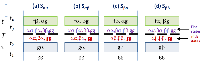
Figure 1: Liouville space pathways corresponding to each of the four resonances in the 2D-ES of a coupled dimer. The amplitude $S_{mn}(T)$ corresponds to the peak located at $(\omega_{\tau},\omega_{t})=(\omega_{mg},\omega_{ng})$, which are the values of the optical frequencies at the coherence and echo time intervals $\tau$ and $t$, respectively. These amplitudes provide information on the coherent and incoherent excitonic processes at the waiting time $T$ by enumerating the possible initial and final states at the waiting time $T$ which satisfy the PE phase matching condition for the pulses acting at times $t_{1},t_{2},t_{3},t_{4}$. The information contained in the amplitudes $S_{mn}(T)$ can be distilled to reconstruct the process matrix for the single-exciton manifold of the dimer, thus allowing for a QPT.

To be more explicit, consider the pathways in $S_{\alpha\beta}(T)$ that monitor the population to coherence process $\chi_{\beta\alpha\alpha\alpha}(T)$. These are displayed in Fig. (2). The pathway on the left involves represents an excited state absorption (ESA) from the single-exciton manifold, and is proportional to $(-C_{\omega_{1}}^{\alpha}\boldsymbol{\mu}_{\alpha g}\cdot\boldsymbol{e}_{1})(C_{\omega_{2}}^{\alpha}\boldsymbol{\mu}_{\alpha g}\cdot\boldsymbol{e}_{2})(C_{\omega_{3}}^{\alpha}\boldsymbol{\mu}_{f\beta}\cdot\boldsymbol{e}_{3})(\boldsymbol{\mu}_{f\alpha}\cdot\boldsymbol{e}_{4})$, an expression which can be immediately read out from the diagram: Each interaction with the field picks up a factor corresponding to the amplitude of the transition, which depends on the alignment of the corresponding dipole with the polarization of the pulse, as well as the frequency amplitude of the pulse at the given transition. A minus sign is included if the perturbation is on the bra. Similarly, the pathway on the right involves stimulated emission (SE) and is proportional to $(-C_{\omega_{1}}^{\alpha}\boldsymbol{\mu}_{\alpha g}\cdot\boldsymbol{e}_{1})(C_{\omega_{2}}^{\alpha}\boldsymbol{\mu}_{\alpha g}\cdot\boldsymbol{e}_{2})(-C_{\omega_{3}}^{\alpha}\boldsymbol{\mu}_{\alpha g}\cdot\boldsymbol{e}_{3})(\boldsymbol{\mu}_{\beta g}\cdot\boldsymbol{e}_{4})$.

The rest of the diagrams for all the peaks can be systematically analyzed in the way described above. In general, the pathways we need to consider can be classified in ESA, SE, and ground state bleaching (GSB) processes. GSB processes are the ones that take $|g\rangle\langle g|$ at the end of the waiting time to a dipole active coherence involving an excited state. ESA pathways, which are proportional to dipole transitions involving the excited state, differ in sign from SE and GSB pathways, as can be easily seen by inspection.

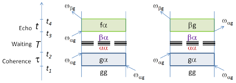
Figure 2: A more detailed view on the Liouville space pathways corresponding to the monitoring of the population to coherence process $\chi_{\beta\alpha\alpha\alpha}(T)$ in the peak at $(\omega_{\tau},\omega_{t})=(\omega_{\alpha g},\omega_{\beta g})$ of the 2D-ES. These diagrams belong to the amplitude $S_{\alpha\beta}(T)$ and can be easy constructed by taking into account the PE phase-matching and the resonant conditions.

Fig. (3) provides a mnemonic device to keep track of the Liouville pathways that each peak in the 2D electronic spectrum monitors, and therefore, also provides a scheme of the QPT protocol. The $\omega_{\tau}$ axis can be associated with a particular state preparation whereas the $\omega_{t}$ axis with a particular detection. Each peak reflects a nontrivial number of processes in Liouville space. As an illustration (see Fig. (4)), we consider the ideal case where the bath does not interact with the system, in which case, a very simple picture is recovered: The off-diagonal peaks beat at the coherence frequency and the diagonals remain static. This case can be easily derived from Eqs. (35), (36), (37), and (38) by substituting $\chi_{abcd}(T)=\delta_{ab}\delta_{cd}+\delta_{ac}\delta_{bd}e^{-i\omega_{ab}T}$, that is, populations remain static whereas coherences beat at difference frequencies.

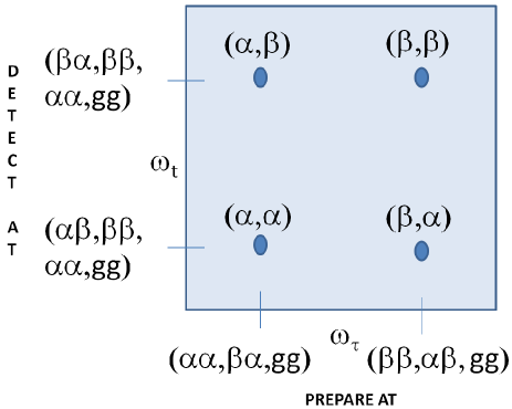
Figure 3: Summary of QPT for a coupled dimer in the 2D-ES. The Liouville pathways depicted in Fig. 1 can be condensed into this diagram. The horizontal axis for the coherence frequency $\omega_{\tau}$ is associated with a state preparation, whereas the vertical axis for the echo frequency $\omega_{t}$ corresponds to a detection. The four resonances labeled as $(m,n)$ correspond to peaks located at $(\omega_{\tau},\omega_{t})=(\omega_{mg},\omega_{ng})$. Their amplitudes contain information on $\chi_{abcd}(T)$, where $cd$ is the state prepared at the beginning of the waiting time interval, and $ab$ the state detected at the end of the same interval. For instance, the peak at $(\omega_{\alpha},\omega_{\beta})$ keeps track of the elements $\chi_{abcd}(T)$ where $|c\rangle\langle d|\in\{|\alpha\rangle\langle\alpha|,|\beta\rangle\langle\alpha|,|g\rangle\langle g|\}$ and $|a\rangle\langle b|\in\{|\beta\rangle\langle\alpha|,|\beta\rangle\langle\beta|,|\alpha\rangle\langle\alpha|,|g\rangle\langle g|\}$.

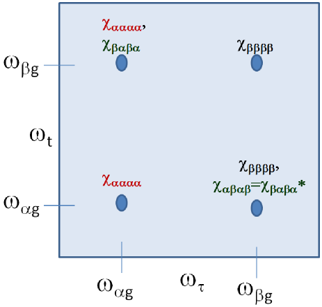
Figure 4: 2D-ES of a coupled dimer in the absence of interactions with a bath. Under unitary dynamics of the excitonic system, each of the four resonances keep track of the elements of $\chi(T)$ indicated in the diagram. Notice that diagonal peaks do not oscillate as a function of waiting time $T$, whereas off-diagonals beat at the frequency equal to the difference in energies of the single exciton eigenstates.

V The case of the homodimer

To gain insights into the described QPT protocol, we specialize the results above to a coupled homodimer. In the following subsections, we discuss, for this particular case, (A) the Hamiltonian and the transition dipole moments involved in the experiments, (B) properties of the spectroscopic signals under isotropic averaging, (C) stability of the numerical inversion, (D) analytical expressions of the elements of $\chi(T)$ in terms of the peak amplitudes of the spectra, (E) a procedure to extract the angle $\phi$ between the dipoles, (F) a summary of the QPT procedure, and (G) a numerical example with a model system. A similar study focused on the heterodimer will be presented in the second part of this series.

V.1 Hamiltonian and transition dipole moments

In the homodimer, the two sites are identical chromophores with energies $\omega_{A}=\omega_{B}=\bar{\omega}$, and the Hamiltonian in Eq. (5) and (7) is given by:

$$H_{S} = \bar{\omega}(a_{A}^{+}a_{A}+a_{B}^{+}a_{B})+J(a_{A}^{+}a_{B}+a_{B}^{+}a_{A})$$ (50)

$$= (\bar{\omega}-J)a_{\alpha}^{+}a_{\alpha}+(\bar{\omega}+J)a_{\beta}^{+}a_{\beta},$$

which we have diagonalized with the symmetric $a_{\beta}^{+}|g\rangle$ and antisymmetric $a_{\alpha}^{+}|g\rangle$ single exciton states given by:

$$a_{\alpha}^{+} = \frac{1}{\sqrt{2}}(a_{A}^{+}+a_{B}^{+}),$$

$$a_{\beta}^{+} = \frac{1}{\sqrt{2}}(a_{A}^{+}-a_{B}^{+}).$$ (51)

The splitting between the two delocalized states is just $2J$. Using Eq. (23), the transition dipoles take the simple forms:

$$\boldsymbol{\mu}_{\alpha g} = \frac{1}{\sqrt{2}}(\boldsymbol{d}_{A}+\boldsymbol{d}_{B}),$$

$$\boldsymbol{\mu}_{\beta g} = \frac{1}{\sqrt{2}}(\boldsymbol{d}_{A}-\boldsymbol{d}_{B}),$$

$$\boldsymbol{\mu}_{f\alpha} = \boldsymbol{\mu}_{\alpha g},$$

$$\boldsymbol{\mu}_{f\beta} = -\boldsymbol{\mu}_{\beta g}.$$ (52)

Interestingly, these expressions are independent of the coupling $J$. Also, notice that $\boldsymbol{\mu}_{\alpha g}$ and $\boldsymbol{\mu}_{f\alpha}$ are perpendicular to $\boldsymbol{\mu}_{\beta g}$ and $\boldsymbol{\mu}_{f\beta}$ (see Fig. 5). Denoting the norm of each site dipole by

$$|\boldsymbol{d}_{A}| = |\boldsymbol{d}_{B}|=d,$$ (53)

the following relationships follow:

$$|\boldsymbol{\mu}_{\alpha g}| = |\boldsymbol{\mu}_{f\alpha}|=\mu_{\alpha g}=\sqrt{2}d\cos\left(\frac{\phi}{2}\right),$$

$$|\boldsymbol{\mu}_{\beta g}| = |\boldsymbol{\mu}_{f\beta}|=\mu_{\beta g}=\sqrt{2}d\sin\left(\frac{\phi}{2}\right).$$ (54)

As expected, in the degenerate limit that $\phi=0$ or $\pi$ (the site dipoles are parallel or antiparallel), one of the delocalized excitons becomes dark and there is only one bright transition from the ground state. If this is not the case, in general, the two transitions are bright and their dipoles perpendicular to each other. Furthermore, as a difference with the heterodimer case, there are only three (instead of four) different transition dipoles in the homodimer, and two of them are just negatives of each other. The degenerate case will be discussed as a limit of the more general one in the next paragraphs.

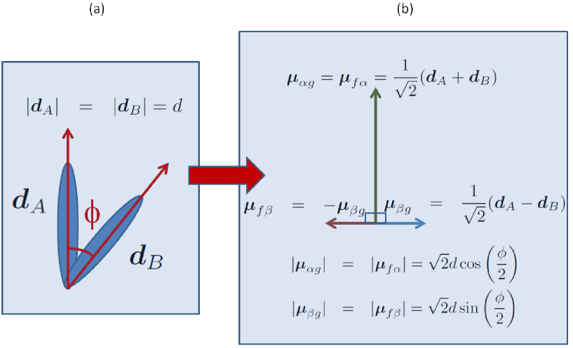
Figure 5: Transition dipole moments of a homodimer. Diagrams for (a) sites and (b) eigenstates.

V.2 Isotropic averaging of signals

An important observation regarding isotropic averaging follows:

Claim.– Upon isotropic averaging, signals stemming from coherence to population or population to coherence transfer cannot be monitored in the 2D-PE spectrum of a homodimer.

Proof.– For simplicity, align $\boldsymbol{\mu}_{\beta g}$ and $\boldsymbol{\mu}_{\alpha g}$ in the $\boldsymbol{y}$ and $\boldsymbol{z}$ directions in the frame of the molecule and use Eq. (39) to argue that the only terms in the sum that contribute to an isotropic averaging are the ones where only two or four polarizations of the field are the same. In Eqs. (35), (36), (37), and (38), all the dipole-polarization terms corresponding to coherence to population and the opposite processes involve three dipoles of the same kind and a perpendicular one. Therefore, they vanish under isotropic averaging. As an example, consider the the terms associated with $\chi_{\beta\alpha\alpha\alpha}(T)$ in $S_{\alpha\beta}(T)$:

$$\langle(-C_{\omega_{1}}^{\alpha}\boldsymbol{\mu}_{\alpha g}\cdot\boldsymbol{e}_{1})(C_{\omega_{2}}^{\alpha}\boldsymbol{\mu}_{\alpha g}\cdot\boldsymbol{e}_{2})(C_{\omega_{3}}^{\alpha}\boldsymbol{\mu}_{f\beta}\cdot\boldsymbol{e}_{3})(\boldsymbol{\mu}_{f\alpha}\cdot\boldsymbol{e}_{4})\rangle$$

$$\propto \langle(\boldsymbol{\mu}_{\alpha g}\cdot\boldsymbol{e}_{1})(\boldsymbol{\mu}_{\alpha g}\cdot\boldsymbol{e}_{2})(\boldsymbol{\mu}_{\beta g}\cdot\boldsymbol{e}_{3})(\boldsymbol{\mu}_{\alpha g}\cdot\boldsymbol{e}_{4})\rangle_{iso}$$

$$= 0,$$

$$(\langle-C_{\omega_{1}}^{\alpha}\boldsymbol{\mu}_{\alpha g}\cdot\boldsymbol{e}_{1})(C_{\omega_{2}}^{\alpha}\boldsymbol{\mu}_{\alpha g}\cdot\boldsymbol{e}_{2})(-C_{\omega_{3}}^{\alpha}\boldsymbol{\mu}_{\alpha g}\cdot\boldsymbol{e}_{3})(\boldsymbol{\mu}_{\beta g}\cdot\boldsymbol{e}_{4})\rangle$$

$$\propto \langle(\boldsymbol{\mu}_{\alpha g}\cdot\boldsymbol{e}_{1})(\boldsymbol{\mu}_{\alpha g}\cdot\boldsymbol{e}_{2})(\boldsymbol{\mu}_{\alpha g}\cdot\boldsymbol{e}_{3})(\boldsymbol{\mu}_{\beta g}\cdot\boldsymbol{e}_{4})\rangle$$

$$= 0.$$

$\Box$

The claim above allows for a considerable simplification of Eqs. (35), (36), (37), and (38). Each of the peaks in the 2D spectrum keeps track of less elements of the process matrix $\chi(T)$ upon isotropic averaging: Only population to population and coherence to coherence transfers can be monitored. The results for the peaks of an isotropically averaged 2D spectra are presented below. We have taken the shortcut notation $\langle\cdot\rangle_{e_{1}e_{2}e_{3}e_{4}}$, which denotes the isotropically averaged signal stemming from the two pulse polarization configurations $(\boldsymbol{e}_{1},\boldsymbol{e}_{2},\boldsymbol{e}_{3},\boldsymbol{e}_{4})=(\boldsymbol{z},\boldsymbol{z},\boldsymbol{z},\boldsymbol{z}),(\boldsymbol{z},\boldsymbol{z},\boldsymbol{x},\boldsymbol{x})$, so that the terms $\langle S_{mn}(T)\rangle_{e_{1}e_{2}e_{3}e_{4}}$ and $\langle S(\omega_{\tau},T,\omega_{t})\rangle_{e_{1}e_{2}e_{3}e_{4}}$ have the obvious meanings.

TABLE 1. Isotropically averaged 2D-ES peak amplitudes for the $\boldsymbol{z}\boldsymbol{z}\boldsymbol{z}\boldsymbol{z}$ configuration
$\displaystyle\langle S_{\alpha\beta}(T)\rangle_{zzzz}$ $\displaystyle=$ $\displaystyle-iC_{\omega_{1}}^{\alpha}C_{\omega_{2}}^{\alpha}C_{\omega_{3}}^{\beta}$ $\displaystyle\times[\frac{1}{15}\mu_{\alpha g}^{2}\mu_{\beta g}^{2}(\chi_{gg\alpha\alpha}(T)-1-\chi_{\beta\beta\alpha\alpha}(T))$ $\displaystyle+\frac{1}{5}\mu_{\alpha g}^{4}\chi_{\alpha\alpha\alpha\alpha}(T)]$ $\displaystyle-iC_{\omega_{1}}^{\alpha}C_{\omega_{2}}^{\beta}C_{\omega_{3}}^{\alpha}[(-)\frac{2}{15}\mu_{\alpha g}^{2}\mu_{\beta g}^{2}\chi_{\beta\alpha\beta\alpha}(T)]$	$\displaystyle\langle S_{\beta\beta}(T)\rangle_{zzzz}$ $\displaystyle=$ $\displaystyle-iC_{\omega_{1}}^{\beta}C_{\omega_{2}}^{\beta}C_{\omega_{3}}^{\beta}$ $\displaystyle\times[\frac{1}{5}\mu_{\beta g}^{4}(\chi_{gg\beta\beta}(T)-1-\chi_{\beta\beta\beta\beta}(T))$ $\displaystyle+\frac{1}{15}\mu_{\beta g}^{2}\mu_{\alpha g}^{2}\chi_{\alpha\alpha\beta\beta}(T)]$ $\displaystyle-iC_{\omega_{1}}^{\beta}C_{\omega_{2}}^{\alpha}C_{\omega_{3}}^{\alpha}[(-)\frac{2}{15}\mu_{\beta g}^{2}\mu_{\alpha g}^{2}\chi_{\beta\alpha\alpha\beta}(T)]$
$\displaystyle\langle S_{\alpha\alpha}(T)\rangle_{zzzz}$ $\displaystyle=$ $\displaystyle-iC_{\omega_{1}}^{\alpha}C_{\omega_{2}}^{\alpha}C_{\omega_{3}}^{\alpha}$ $\displaystyle\times[\frac{1}{5}\mu_{\alpha g}^{4}(\chi_{gg\alpha\alpha}(T)-1-\chi_{\alpha\alpha\alpha\alpha}(T))$ $\displaystyle+\frac{1}{15}\mu_{\alpha g}^{2}\mu_{\beta g}^{2}\chi_{\beta\beta\alpha\alpha}(T)]$ $\displaystyle-iC_{\omega_{1}}^{\alpha}C_{\omega_{2}}^{\beta}C_{\omega_{3}}^{\beta}[(-)\frac{2}{15}\mu_{\alpha g}^{2}\mu_{\beta g}^{2}\chi_{\alpha\beta\beta\alpha}(T)]$	$\displaystyle\langle S_{\beta\alpha}(T)\rangle_{zzzz}$ $\displaystyle=$ $\displaystyle-iC_{\omega_{1}}^{\beta}C_{\omega_{2}}^{\beta}C_{\omega_{3}}^{\alpha}$ $\displaystyle\times[\frac{1}{15}\mu_{\beta g}^{2}\mu_{\alpha g}^{2}(\chi_{gg\beta\beta}(T)-1-\chi_{\alpha\alpha\beta\beta}(T))$ $\displaystyle+\frac{1}{5}\mu_{\beta g}^{4}\chi_{\beta\beta\beta\beta}(T)]$ $\displaystyle-iC_{\omega_{1}}^{\beta}C_{\omega_{2}}^{\alpha}C_{\omega_{3}}^{\beta}[(-)\frac{2}{15}\mu_{\beta g}^{2}\mu_{\alpha g}^{2}\chi_{\alpha\beta\alpha\beta}(T)]$

TABLE 2. Isotropically averaged 2D-ES peak amplitudes for the $\boldsymbol{z}\boldsymbol{z}\boldsymbol{x}\boldsymbol{x}$ configuration
$\displaystyle\langle S{}_{\alpha\beta}(T)\rangle_{zzxx}$ $\displaystyle=$ $\displaystyle-iC_{\omega_{1}}^{\alpha}C_{\omega_{2}}^{\alpha}C_{\omega_{3}}^{\beta}$ $\displaystyle\times[\frac{2}{15}\mu_{\alpha g}^{2}\mu_{\beta g}^{2}(\chi_{gg\alpha\alpha}(T)-1-\chi_{\beta\beta\alpha\alpha}(T))$ $\displaystyle+\frac{1}{15}\mu_{\alpha g}^{4}\chi_{\alpha\alpha\alpha\alpha}(T)]$ $\displaystyle-iC_{\omega_{1}}^{\alpha}C_{\omega_{2}}^{\beta}C_{\omega_{3}}^{\alpha}[(+)\frac{1}{15}\mu_{\alpha g}^{2}\mu_{\beta g}^{2}\chi_{\beta\alpha\beta\alpha}(T)]$	$\displaystyle\langle S_{\beta\beta}(T)\rangle_{zzxx}$ $\displaystyle=$ $\displaystyle-iC_{\omega_{1}}^{\beta}C_{\omega_{2}}^{\beta}C_{\omega_{3}}^{\beta}$ $\displaystyle\times[\frac{1}{15}\mu_{\beta g}^{4}(\chi_{gg\beta\beta}(T)-1-\chi_{\beta\beta\beta\beta}(T))$ $\displaystyle+\frac{2}{15}\mu_{\beta g}^{2}\mu_{\alpha g}^{2}\chi_{\alpha\alpha\beta\beta}(T)]$ $\displaystyle-iC_{\omega_{1}}^{\beta}C_{\omega_{2}}^{\alpha}C_{\omega_{3}}^{\alpha}[(+)\frac{1}{15}\mu_{\beta g}^{2}\mu_{\alpha g}^{2}\chi_{\beta\alpha\alpha\beta}(T)]$
$\displaystyle\langle S_{\alpha\alpha}(T)\rangle_{zzxx}$ $\displaystyle=$ $\displaystyle-iC_{\omega_{1}}^{\alpha}C_{\omega_{2}}^{\alpha}C_{\omega_{3}}^{\alpha}$ $\displaystyle\times[\frac{1}{15}\mu_{\alpha g}^{4}(\chi_{gg\alpha\alpha}(T)-1-\chi_{\alpha\alpha\alpha\alpha}(T))$ $\displaystyle+\frac{2}{15}\mu_{\alpha g}^{2}\mu_{\beta g}^{2}\chi_{\beta\beta\alpha\alpha}(T)]$ $\displaystyle-iC_{\omega_{1}}^{\alpha}C_{\omega_{2}}^{\beta}C_{\omega_{3}}^{\beta}[(+)\frac{1}{15}\mu_{\alpha g}^{2}\mu_{\beta g}^{2}\chi_{\alpha\beta\beta\alpha}(T)]$	$\displaystyle\langle S_{\beta\alpha}(T)\rangle_{zzxx}$ $\displaystyle=$ $\displaystyle-iC_{\omega_{1}}^{\beta}C_{\omega_{2}}^{\beta}C_{\omega_{3}}^{\alpha}$ $\displaystyle\times[\frac{2}{15}\mu_{\beta g}^{2}\mu_{\alpha g}^{2}(\chi_{gg\beta\beta}(T)-1-\chi_{\alpha\alpha\beta\beta}(T))$ $\displaystyle+\frac{1}{15}\mu_{\beta g}^{4}\chi_{\beta\beta\beta\beta}(T)]$ $\displaystyle-iC_{\omega_{1}}^{\beta}C_{\omega_{2}}^{\alpha}C_{\omega_{3}}^{\beta}[(+)\frac{1}{15}\mu_{\beta g}^{2}\mu_{\alpha g}^{2}\chi_{\alpha\beta\alpha\beta}(T)]$

We focus our attention on experiments with short pulses that are broadband enough to create either exciton $|\alpha\rangle$ or $|\beta\rangle$ with the same amplitude, that is, $C_{\omega_{i}}^{p}=C$, for a purely imaginary constant $C$, for all $p$ and $\omega_{i}$. This condition can be easily relaxed, but we shall proceed with it to analyze our QPT protocol with more detail. Using the condition of Eq. (3), we can eliminate the variables $\chi_{gg\alpha\alpha}(T)$ and $\chi_{gg\beta\beta}(T)$ for $\chi_{\alpha\alpha\alpha\alpha}(T),\chi_{\beta\beta\alpha\alpha}(T),\chi_{\alpha\alpha\beta\beta}(T),\chi_{\beta\beta\beta\beta}(T)$. Also, taking advantage of Eq. (4), we discard $\chi_{\beta\alpha\beta\alpha}(T)$ and $\chi_{\alpha\beta\beta\alpha}(T)$ and keep $\chi_{\alpha\beta\alpha\beta}(T)$ and $\chi_{\beta\alpha\alpha\beta}(T)$. From the left hand side (LHS) of the real and imaginary parts of the spectrum (see Tables 1 and 2), we derive the following real valued matrix equation:

$$iC^{3}\left[\begin{array}[]{cccccc}\frac{2}{5}\mu_{\alpha g}^{4}&\frac{1}{5}\mu_{\alpha g}^{4}-\frac{1}{15}\mu_{\alpha g}^{2}\mu_{\beta g}^{2}&0&\frac{2}{15}\mu_{\alpha g}^{2}\mu_{\beta g}^{2}&0&0\\ \frac{2}{15}\mu_{\alpha g}^{4}&\frac{1}{15}\mu_{\alpha g}^{4}-\frac{2}{15}\mu_{\alpha g}\mu_{\beta g}^{2}&0&-\frac{1}{15}\mu_{\alpha g}^{2}\mu_{\beta g}^{2}&0&0\\ -\frac{1}{5}\mu_{\alpha g}^{4}+\frac{1}{15}\mu_{\alpha g}^{2}\mu_{\beta g}^{2}&\frac{2}{15}\mu_{\alpha g}^{2}\mu_{\beta g}^{2}&\frac{2}{15}\mu_{\alpha g}^{2}\mu_{\beta g}^{2}&0&0&0\\ -\frac{1}{15}\mu_{\alpha g}^{4}+\frac{2}{15}\mu_{\alpha g}^{2}\mu_{\beta g}^{2}&\frac{4}{15}\mu_{\alpha g}^{2}\mu_{\beta g}^{2}&-\frac{1}{15}\mu_{\alpha g}^{2}\mu_{\beta g}^{2}&0&0&0\\ 0&0&0&0&0&-\frac{2}{15}\mu_{\alpha g}^{2}\mu_{\beta g}^{2}\\ 0&0&0&0&0&\frac{1}{15}\mu_{\alpha g}^{2}\mu_{\beta g}^{2}\\ 0&0&0&0&-\frac{2}{15}\mu_{\alpha g}^{2}\mu_{\beta g}^{2}&0\\ 0&0&0&0&\frac{1}{15}\mu_{\alpha g}^{2}\mu_{\beta g}^{2}&0\end{array}\right]\left[\begin{array}[]{c}\chi_{\alpha\alpha\alpha\alpha}(T)\\ \chi_{\beta\beta\alpha\alpha}(T)\\ \Re\{\chi_{\alpha\beta\alpha\beta}(T)\}\\ \Re\{\chi_{\beta\alpha\alpha\beta}(T)\}\\ \Im\{\chi_{\alpha\beta\alpha\beta}(T)\}\\ \Im\{\chi_{\beta\alpha\alpha\beta}(T)\}\end{array}\right] = \left[\begin{array}[]{c}\Re\{\langle S_{\alpha\alpha}(T)\rangle_{zzzz}\}\\ \Re\{\langle S_{\alpha\alpha}(T)\rangle_{zzxx}\}\\ \Re\{\langle S_{\alpha\beta}(T)\rangle_{zzzz}\}\\ \Re\{\langle S_{\alpha\beta}(T)\rangle_{zzxx}\}\\ \Im\{\langle S_{\alpha\alpha}(T)\rangle_{zzzz}\}\\ \Im\{\langle S_{\alpha\alpha}(T)\rangle_{zzxx}\}\\ \Im\{\langle S_{\alpha\beta}(T)\rangle_{zzzz}\}\\ \Im\{\langle S_{\alpha\beta}(T)\rangle_{zzxx}\}\end{array}\right].$$ (77)

Similarly, the right hand side (RHS) of the spectra yields:

$$iC^{3}\left[\begin{array}[]{cccccc}\frac{2}{5}\mu_{\beta g}^{4}&\frac{1}{5}\mu_{\beta g}^{4}-\frac{1}{15}\mu_{\beta g}^{2}\mu_{\alpha g}^{2}&0&\frac{2}{15}\mu_{\beta g}^{2}\mu_{\alpha g}^{2}&0&0\\ \frac{2}{15}\mu_{\beta g}^{4}&\frac{1}{15}\mu_{\beta g}^{4}-\frac{2}{15}\mu_{\beta g}\mu_{\alpha g}^{2}&0&-\frac{1}{15}\mu_{\beta g}^{2}\mu_{\alpha g}^{2}&0&0\\ -\frac{1}{5}\mu_{\beta g}^{4}+\frac{1}{15}\mu_{\beta g}^{2}\mu_{\alpha g}^{2}&\frac{2}{15}\mu_{\beta g}^{2}\mu_{\alpha g}^{2}&\frac{2}{15}\mu_{\beta g}^{2}\mu_{\alpha g}^{2}&0&0&0\\ -\frac{1}{15}\mu_{\beta g}^{4}+\frac{2}{15}\mu_{\beta g}^{2}\mu_{\alpha g}^{2}&\frac{4}{15}\mu_{\beta g}^{2}\mu_{\alpha g}^{2}&-\frac{1}{15}\mu_{\beta g}^{2}\mu_{\alpha g}^{2}&0&0&0\\ 0&0&0&0&0&\frac{2}{15}\mu_{\beta g}^{2}\mu_{\alpha g}^{2}\\ 0&0&0&0&0&-\frac{1}{15}\mu_{\beta g}^{2}\mu_{\alpha g}^{2}\\ 0&0&0&0&\frac{2}{15}\mu_{\beta g}^{2}\mu_{\alpha g}^{2}&0\\ 0&0&0&0&-\frac{1}{15}\mu_{\beta g}^{2}\mu_{\alpha g}^{2}&0\end{array}\right]\left[\begin{array}[]{c}\chi_{\beta\beta\beta\beta}(T)\\ \chi_{\alpha\alpha\beta\beta}(T)\\ \Re\{\chi_{\alpha\beta\alpha\beta}(T)\}\\ \Re\{\chi_{\beta\alpha\alpha\beta}(T)\}\\ \Im\{\chi_{\alpha\beta\alpha\beta}(T)\}\\ \Im\{\chi_{\beta\alpha\alpha\beta}(T)\}\end{array}\right] = \left[\begin{array}[]{c}\Re\{\langle S_{\beta\beta}(T)\rangle_{zzzz}\}\\ \Re\{\langle S_{\beta\beta}(T)\rangle_{zzxx}\}\\ \Re\{\langle S_{\beta\alpha}(T)\rangle_{zzzz}\}\\ \Re\{\langle S_{\beta\alpha}(T)\rangle_{zzxx}\}\\ \Im\{\langle S_{\beta\beta}(T)\rangle_{zzzz}\}\\ \Im\{\langle S_{\beta\beta}(T)\rangle_{zzxx}\}\\ \Im\{\langle S_{\beta\alpha}(T)\rangle_{zzzz}\}\\ \Im\{\langle S_{\beta\alpha}(T)\rangle_{zzxx}\}\end{array}\right].$$ (100)

Inverting Eqs. (77) and (100) yields most of the elements of $\chi(T)$ involving the single-exciton manifold. Whereas the presented QPT for the homodimer is partial, no complicated pulse shaping efforts need to be carried out. Instead, the requirement is standard pulse polarization control achievable with current experimental capabilities woutersen ; perakis ; zanni-njp ; khalil:362 ; khaliljpc ; moran-polarization ; moran-polarization-ii ; Schlau-Cohen27072010 .

The transition dipole moments must be well characterized in order to construct the matrices in Eqs. (77) and (100). This requirement is self-consistently fulfilled by collecting the spectra in the collinear and cross-polarized configurations. Notice that $\chi_{\alpha\alpha\alpha\alpha}(T)$ and $\chi_{\beta\beta\alpha\alpha}(T)$ are exclusively monitored in the LHS, and $\chi_{\beta\beta\beta\beta}(T)$ and $\chi_{\alpha\alpha\beta\beta}(T)$ only detected in the RHS. However, coherence transfer terms $\chi_{\alpha\beta\alpha\beta}(T)$ and $\chi_{\beta\alpha\alpha\beta}(T)$ are repeatedly monitored in different peaks in both sides of the spectra. Due to this repetition, there are redudant equations that allow for the self-consistent extraction of the angle $\phi$ without compromising the inversion of the elements of $\chi(T)$. Details about this parameter extraction are developed in subsection E. For the time being, we assume that the information about the transition dipoles is previously known.

V.3 Stability of the Quantum Process Tomography protocol for a homodimer

In order to characterize the stability of inversion of $\chi(T)$, we can arrange Eqs. (77) and (100) into a single matrix equation $\boldsymbol{M}\vec{\chi}(T)=\vec{S}(T)$, where $\boldsymbol{M}$ is a $16\times 8$ matrix of dipole moments, $\vec{\chi}(T)$ is a vector of 8 unknowns, and $\vec{S}(T)$ is a vector of 16 real valued amplitudes extracted from the signal. Denoting with $\parallel\cdot\parallel$ the spectral norm of a vector or a matrix numerical , we obtain a bound on the relative error of the inverted vector $\vec{\chi}(T)$ which yields the QPT:

$$\frac{||\Delta\vec{\chi}(T)||}{||\vec{\chi}(T)||}\leq\kappa\frac{\parallel\Delta S(T)\parallel}{\parallel S(T)\parallel},$$ (101)

where $\Delta\vec{\chi}(T)$ and $\Delta S(T)$ denote errors in $\vec{\chi}(T)$ and $S(T)$ upon inversion, respectively, and the condition number $\kappa$ is given by:

$$\kappa=\parallel\boldsymbol{M}\parallel\parallel\boldsymbol{M}^{-1}\parallel$$ (102)

The lowest possible value for a condition number is $\kappa=1$. In Fig. (6), a plot of $\kappa$ vs. $\phi$ (red) is displayed. As expected, very large values of $\kappa$, which denote unstable inversions, are expected for systems where the site dipoles are aligned or antialigned, when one of the eigenstates of $H_{S}$ becomes dark. We also indicate a range of angles where $\kappa$ is below a reasonable threshold, say $\kappa\leq 15$ (blue horizontal line), which consists of angles in the range $0.3\pi\leq\phi\leq 0.7\pi$. Also, note that $\kappa$ is symmetric about the minimum of $\kappa$ at $\phi=\pi/2$, where the best inversion is carried out with $\kappa\sim 3.9$.

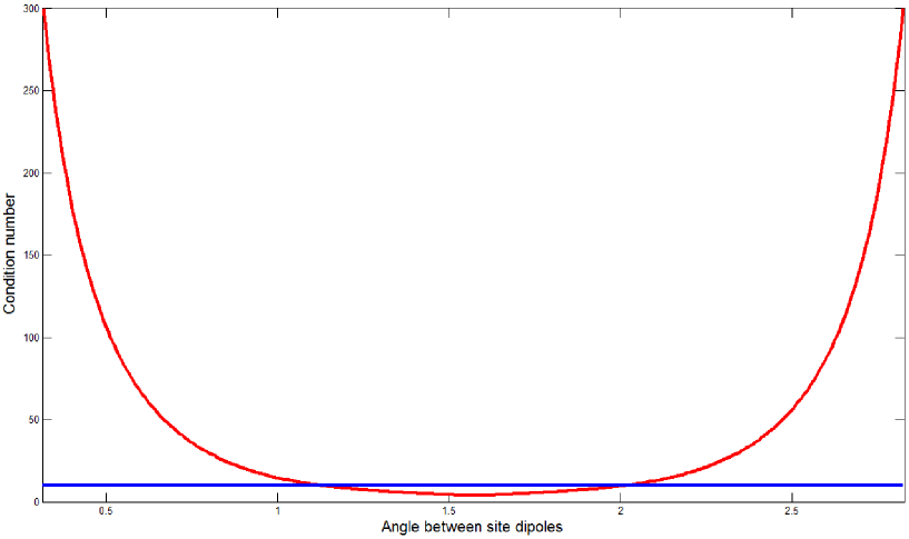
Figure 6: Stability of the homodimer QPT protocol. As described in the text, the QPT protocol depends on the inversion of a matrix which is a function of transition dipole moments. The condition number of the matrix ($\kappa$) vs. the angle between site dipoles ($\phi$) is plotted in red. The blue line plots the constant value of $\kappa=15$, as a reference to indicate that for the range of angles $0.3\pi\leq\phi\leq 0.7\pi$, the condition number is below that value.

V.4 Analytical expressions for $\chi(T)$

To gain insights into the QPT protocol, we shall derive explicit expressions for the elements of $\chi(T)$ in terms of the amplitudes of the spectra and the angle $\phi$ between the dipoles. First, we substitute Eqs. (53) and (54) into the LHS of the spectra through Eq. (77). The following expressions are obtained after inverting the resulting matrix equation:

$$\chi_{gg\alpha\alpha}(T)-1 = -\frac{\sec^{2}(\phi/2)}{(iC^{3})(20d^{4})}$$ (103)

$$\times\Re\{\langle S_{\alpha\alpha}(T)\rangle_{zzzz}+2\langle S_{\alpha\alpha}(T)\rangle_{zzxx}$$

$$+\langle S_{\alpha\beta}(T)\rangle_{zzzz}+2\langle S_{\alpha\beta}(T)\rangle_{zzxx}\}$$

$$\chi_{\alpha\alpha\alpha\alpha}(T) = -\frac{\sec^{2}(\phi/2)}{(iC^{3})(20d^{4})}$$ (104)

$$\times\Re\{(\cos\phi-1)(\langle S_{\alpha\alpha}(T)\rangle_{zzzz}+2\langle S_{\alpha\alpha}(T)\rangle_{zzxx}$$

$$+\cos\phi(\langle S_{\alpha\beta}(T)\rangle_{zzzz}+2\langle S_{\alpha\beta}(T)\rangle_{zzxx})\}$$

‘

$$\chi_{\beta\beta\alpha\alpha}(T) = \frac{\sec^{2}(\phi/2)}{(iC^{3})(20d^{4})}$$ (105)

$$\times\Re\{\cos\phi(\langle S_{\alpha\alpha}(T)\rangle_{zzzz}+2\langle S_{\alpha\alpha}(T)\rangle_{zzxx})$$

$$+(\cos\phi+1)(\langle S_{\alpha\beta}(T)\rangle_{zzzz}+2\langle S_{\alpha\beta}(T)\rangle_{zzxx})\}$$

$$\Re\{\chi_{\alpha\beta\alpha\beta}(T)\} = \frac{1}{(iC^{3})(20d^{4})}$$ (106)

$$\times\Re\{2(\langle S_{\alpha\alpha}(T)\rangle_{zzzz}+2\langle S_{\alpha\alpha}(T)\rangle_{zzxx})$$

$$+(\cot^{2}\frac{\phi}{2}+2\tan^{2}\frac{\phi}{2}+5)\langle S_{\alpha\beta}(T)\rangle_{zzzz}$$

$$-(3\cot^{2}\frac{\phi}{2}+\tan^{2}\frac{\phi}{2})\langle S_{\alpha\beta}(T)\rangle_{zzxx}\}$$

$$\Re\{\chi_{\beta\alpha\alpha\beta}(T)\} = \frac{1}{(iC^{3})(20d^{4})}$$ (107)

$$\times\Re\{(\cot^{2}\frac{\phi}{2}+2\tan^{2}\frac{\phi}{2}+1)\langle S_{\alpha\alpha}(T)\rangle_{zzzz}$$

$$-(3\cot^{2}\frac{\phi}{2}+\tan^{2}\frac{\phi}{2}+8)\langle S_{\alpha\alpha}(T)\rangle_{zzxx}$$

$$-2(\langle S_{\alpha\beta}(T)\rangle_{zzzz}+2\langle S_{\alpha\beta}(T)\rangle_{zzxx})\}$$

$$\Im\{\chi_{\alpha\beta\alpha\beta}(T)\} = \frac{15}{(iC^{3})(8d^{4})}\Im\{(\csc^{2}\frac{\phi}{2}\sec^{2}\frac{\phi}{2})\langle S_{\alpha\beta}(T)\rangle_{zzzz}\}$$ (108)

$$= -\frac{15}{(iC^{3})(4d^{4})}\Im\{(\csc^{2}\frac{\phi}{2}\sec^{2}\frac{\phi}{2})\langle S_{\alpha\beta}(T)\rangle_{zzxx}\}$$

$$\Im\{\chi_{\beta\alpha\alpha\beta}(T)\} = \frac{15}{(iC^{3})(8d^{4})}\Im\{(\csc^{2}\frac{\phi}{2}\sec^{2}\frac{\phi}{2})\langle S_{\alpha\alpha}(T)\rangle_{zzzz}\}$$ (109)

$$= -\frac{15}{(iC^{3})(4d^{4})}\Im\{(\csc^{2}\frac{\phi}{2}\sec^{2}\frac{\phi}{2})\langle S_{\alpha\alpha}(T)\rangle_{zzxx}\}$$

Similarly, the RHS of the spectra through Eq. (100) yield:

$$\chi_{gg\beta\beta}(T)-1 = -\frac{\csc^{2}(\phi/2)}{(iC^{3})(20d^{4})}$$ (110)

$$\times\Re\{\langle S_{\beta\beta}(T)\rangle_{zzzz}+2\langle S_{\beta\beta}(T)\rangle_{zzxx}$$

$$+\langle S_{\beta\alpha}(T)\rangle_{zzzz}+2\langle S_{\beta\alpha}(T)\rangle_{zzxx}\}$$

$$\chi_{\beta\beta\beta\beta}(T) = \frac{\csc^{2}(\phi/2)}{(iC^{3})(20d^{4})}$$ (111)

$$\times\Re\{(\cos\phi+1)(\langle S_{\beta\beta}(T)\rangle_{zzzz}+2\langle S_{\beta\beta}(T)\rangle_{zzxx}$$

$$+\cos\phi(\langle S_{\beta\alpha}(T)\rangle_{zzzz}+2\langle S_{\beta\alpha}(T)\rangle_{zzxx})\}$$

‘

$$\chi_{\alpha\alpha\beta\beta}(T) =- \frac{\csc^{2}(\phi/2)}{(iC^{3})(20d^{4})}$$ (112)

$$\times\Re\{\cos\phi(\langle S_{\beta\beta}(T)\rangle_{zzzz}+2\langle S_{\beta\beta}(T)\rangle_{zzxx})$$

$$+(\cos\phi-1)(\langle S_{\beta\alpha}(T)\rangle_{zzzz}+2\langle S_{\beta\alpha}(T)\rangle_{zzxx})\}$$

$$\Re\{\chi_{\alpha\beta\alpha\beta}(T)\} = \frac{1}{(iC^{3})(20d^{4})}$$ (113)

$$\times\Re\{2(\langle S_{\beta\beta}(T)\rangle_{zzzz}+2\langle S_{\beta\beta}(T)\rangle_{zzxx})$$

$$+(\tan^{2}\frac{\phi}{2}+2\cot^{2}\frac{\phi}{2}+5)\langle S_{\beta\alpha}(T)\rangle_{zzzz}$$

$$-(3\tan^{2}\frac{\phi}{2}+\cot^{2}\frac{\phi}{2})\langle S_{\beta\alpha}(T)\rangle_{zzxx}\}$$

$$\Re\{\chi_{\beta\alpha\alpha\beta}(T)\} = \frac{1}{(iC^{3})(20d^{4})}$$ (114)

$$\times\Re\{(\tan^{2}\frac{\phi}{2}+2\cot^{2}\frac{\phi}{2}+1)\langle S_{\beta\beta}(T)\rangle_{zzzz}$$

$$-(3\tan^{2}\frac{\phi}{2}+\cot^{2}\frac{\phi}{2}+8)\langle S_{\beta\beta}(T)\rangle_{zzxx}$$

$$-2(\langle S_{\beta\alpha}(T)\rangle_{zzzz}+2\langle S_{\beta\alpha}(T)\rangle_{zzxx})\}$$

$$\Im\{\chi_{\alpha\beta\alpha\beta}(T)\} = -\frac{15}{(iC^{3})(8d^{4})}\Im\{(\sec^{2}\frac{\phi}{2}\csc^{2}\frac{\phi}{2})\langle S_{\beta\alpha}(T)\rangle_{zzzz}\}$$ (115)

$$= \frac{15}{(iC^{3})(4d^{4})}\Im\{(\sec^{2}\frac{\phi}{2}\csc^{2}\frac{\phi}{2})\langle S_{\beta\alpha}(T)\rangle_{zzxx}\}$$

$$\Im\{\chi_{\beta\alpha\alpha\beta}(T)\} = -\frac{15}{(iC^{3})(8d^{4})}\Im\{(\sec^{2}\frac{\phi}{2}\csc^{2}\frac{\phi}{2})\langle S_{\beta\beta}(T)\rangle_{zzzz}\}$$ (116)

$$= \frac{15}{(iC^{3})(4d^{4})}\Im\{(\sec^{2}\frac{\phi}{2}\csc^{2}\frac{\phi}{2})\langle S_{\beta\beta}(T)\rangle_{zzxx}\}$$

As expected, the RHS equations above can be obtained from the LHS equations upon the substitutions $\alpha\to\beta$, $\beta\to\alpha$, and $\phi\to\pi-\phi$ (see Eqs. (54)).

From Eqs. (108) and (115), we notice that the imaginary parts of $\langle S_{\alpha\beta}(T)\rangle_{zzzz},\langle S_{\alpha\beta}(T)\rangle_{zzxx},\langle S_{\beta\alpha}(T)\rangle_{zzxx},\langle S_{\beta\alpha}(T)\rangle_{zzxx}$ are all exclusively proportional to $\Im\{\chi_{\alpha\beta\alpha\beta}(T)\}$. The least-squares solution for $\Im\{\chi_{\alpha\beta\alpha\beta}(T)\}$ using Eqs. (77) and (100) is simply the average of these four values; the analogous conclusion holds for $\Im\{\chi_{\beta\alpha\alpha\beta}(T)\}$. The real parts, $\Re\{\chi_{\alpha\beta\alpha\beta}(T)\},\Re\{\chi_{\beta\alpha\alpha\beta}(T)\}$ satisfy less trivial relationships. Each of them appears twice in the equations, once in the RHS and another time in the LHS of the spectra. It is this redundancy in the spectral information what allows for the extraction of the angle between the dipoles.

V.5 Determination of the angle $\phi$ between the two dipoles

Equating the values of $\Re\{\chi_{\alpha\beta\alpha\beta}(T)\}$ from the expressions in Eqs. (106) and (113) yield the following quadratic equation in $\xi=\tan^{2}\left(\frac{\phi}{2}\right)$:

$$\Re\{[\langle S_{\beta\alpha}(T)\rangle_{zzzz}-3\langle S_{\beta\alpha}(T)\rangle_{zzxx}-2\langle S_{\alpha\beta}(T)\rangle_{zzzz}+\langle S_{\alpha\beta}(T)\rangle_{zzxx}]\xi^{2}$$ (117)

$$+[5\langle S_{\beta\alpha}(T)\rangle_{zzzz}+2\langle S_{\beta\beta}(T)\rangle_{zzzz}+4\langle S_{\beta\beta}(T)\rangle_{zzxx}$$

$$-5\langle S_{\alpha\beta}(T)\rangle_{zzzz}-2\langle S_{\alpha\alpha}(T)\rangle_{zzzz}-4\langle S_{\alpha\alpha}(T)\rangle_{zzxx}]\xi$$

$$+[2\langle S_{\beta\alpha}(T)\rangle_{zzzz}-\langle S_{\beta\alpha}(T)\rangle_{zzxx}-\langle S_{\alpha\beta}(T)\rangle_{zzzz}+3\langle S_{\alpha\beta}(T)\rangle_{zzxx}]\}$$

$$= 0.$$

A similar expression can be found for $\Re\{\chi_{\beta\alpha\alpha\beta}(T)\}$ from Eqs. (107) and (114):

$$\Re\{[2\langle S_{\alpha\alpha}(T)\rangle_{zzzz}-\langle S_{\alpha\alpha}(T)\rangle_{zzxx}-\langle S_{\beta\beta}(T)\rangle_{zzzz}+3\langle S_{\beta\beta}(T)\rangle_{zzxx}]\xi^{2}$$ (118)

$$+[\langle S_{\alpha\alpha}(T)\rangle_{zzzz}-8\langle S_{\alpha\alpha}(T)\rangle_{zzxx}-2\langle S_{\alpha\beta}(T)\rangle_{zzzz}-4\langle S_{\alpha\beta}(T)\rangle_{zzxx}$$

$$-\langle S_{\beta\beta}(T)\rangle_{zzzz}+8\langle S_{\beta\beta}(T)\rangle_{zzxx}+2\langle S_{\beta\alpha}(T)\rangle_{zzzz}+4\langle S_{\beta\alpha}(T)\rangle_{zzxx}]\xi$$

$$+[\langle S_{\alpha\alpha}(T)\rangle_{zzzz}-3\langle S_{\alpha\alpha}(T)\rangle_{zzxx}-2\langle S_{\beta\beta}(T)\rangle_{zzzz}+\langle S_{\beta\beta}(T)\rangle_{zzxx}]\}$$

$$= 0.$$

The identities in Eqs. (117) and (118) are remarkable in the sense that they are satisfied at every waiting time $T$: they do not depend on short time coherent dynamics. By monitoring the peak amplitudes from the spectra arising from the two different polarization configurations, the angle $\phi$ between the two site dipoles can be readily extracted using either expression. This determination is robust because it can be repeated for every value of $T$ for which the signal has been collected.

V.6 Summary of Quantum Process Tomography protocol for a coupled homodimer

We proceed to summarize the algorithm of the QPT protocol for a coupled homodimer.

1. Obtain the amplitudes $\langle S_{mn}(T)\rangle_{e_{1}e_{2}e_{3}e_{4}}$ for $m,n\in\{\alpha,\beta\}$ and the two polarization settings $(\boldsymbol{e}_{1},\boldsymbol{e}_{2},\boldsymbol{e}_{3},\boldsymbol{e}_{4})=(\boldsymbol{z},\boldsymbol{z},\boldsymbol{z},\boldsymbol{z}),(\boldsymbol{x},\boldsymbol{x},\boldsymbol{z},\boldsymbol{z})$. This information can be extracted from the two respective polarization controlled 2D-ES, $\langle S(\omega_{\tau},T,\omega_{t})\rangle_{e_{1}e_{2}e_{3}e_{4}}$. For simplicity, all the pulses are taken to be of the same duration (short compared to the timescales of excited state dynamics).

2. Extract the angle $\phi$ from the data from step 1 and Eqs. (117) and (118).

3. Plug in information obtained from step 1 and the angle $\phi$ from step 2 into the expressions for the elements of $\chi(T)$ in Eqs. (103)-(116). Some important observations: (a) These expressions are all proportional to the factor $(C^{3}d^{4})^{-1}$. The norm of the dipole $d$ can be extracted from the intensity of the absorption spectrum of the monomer. If this information is not readily available, the results are known up to this constant factor. (b) By construction from Eq. (117), the calculated value of $\Re\{\chi_{\alpha\beta\alpha\beta}(T)\}$ will be the same using either Eqs. (106) or (113). The same holds for Eq. (118), $\Re\{\chi_{\beta\alpha\alpha\beta}(T)\}$ and Eqs. (106) and (113).

V.7 Numerical example

In this subsection, we illustrate the described QPT protocol with a model homodimer. Marcus and coworkers have recently reported a synthetic system of porphyrin molecules which self-assemble into homodimers under the presence of liposomes marcus . The parameters of this system, extracted from phase-modulation electronic coherence spectroscopy (PM-ECS), are $\bar{\omega}=16633\,cm^{-1},$ $J=175\,cm^{-1}$, and $\phi=65^{o}$. The transition energies to the eigenstates are $\omega_{\alpha g}=16458\,cm^{-1}$ and $\omega_{\beta g}=16808\,cm^{-1}$. Information on the spectral density of this system is not available in the literature yet. We adopt a simple system-bath model based on the secular Redfield approach and independent bath approximation (IBA) for each site. The weak system-bath model is reasonable since porphyrins are rigid molecules which change their structures minimally upon electronic excitation. The IBA must be reexamined, since the liposome media guarantee a bosonic bath that could be strongly correlated in both sites. Nevertheless, the purpose of this example is not to provide an exact account of the excited state dynamics of this system, but rather an illustration of the QPT protocol using reasonable timescales that one might encounter in a realistic setting. A careful study of the precise bath-induced dynamics in this system is beyond the scope of this study and shall be addressed in future work in collaboration with an experimental realization.

We consider a harmonic bath with an Ohmic spectral density: $J(\omega)=\frac{\lambda}{\omega_{c}}\omega e^{-\omega/\omega_{c}}$, with $\lambda=100\,cm^{-1}$, $\omega_{c}=150\,cm^{-1}$ at a temperature $T=273\,K$. Identical baths are assumed to be diagonally and linearly coupled to each of the sites. We closely follow the calculation reported in nonperturbativepisliakov and adapted in yuenzhou . The dynamics of the total excitonic system, which is a proper density matrix, is governed by the following equation of motion:

$$\dot{\rho}(T)=-i[H_{S},\rho(T)]-\mathcal{R}\rho(T)$$ (119)

where $\mathcal{R}$ denotes the time-independent sparse dissipative superoperator containing only a few non-zero elements listed in Table 3. Since $\dot{\rho}(T)$ only depends on $\rho(T)$ and not on the value of the quantum state at previous times, the simulated dynamics are Markovian.

TABLE 3. Values (in $fs^{-1}$) of non-zero rates of the secular Redfield tensor
$R_{\beta\beta\alpha\alpha}$	$8.02\times 10^{-4}$
$R_{\alpha\alpha\beta\beta}=e^{-\omega_{\alpha\beta}/k_{B}T}R_{\beta\beta\alpha\alpha}$	$5.07\times 10^{-3}$
$R_{\alpha\beta\alpha\beta}=R_{\beta\alpha\beta\alpha}$	$2.93\times 10^{-3}$
$R_{\alpha g\alpha g}=R_{g\alpha g\alpha}=R_{f\alpha f\alpha}=R_{\alpha f\alpha f}$	$1.23\times 10^{-2}$
$R_{\beta g\beta g}=R_{g\beta g\beta}=R_{f\beta f\beta}=R_{\beta f\beta f}$	$1.45\times 10^{-2}$
$R_{fgfg}=R_{gfgf}$	$4.77\times 10^{-2}$

It is well known that the secular Redfield equations guarantee thermal equilibrium since the population transfer rates satisfy $R_{\alpha\alpha\beta\beta}/R_{\beta\beta\alpha\alpha}=e^{-\omega_{\alpha\beta}/k_{B}T}$, where $k_{B}$ is the Boltzmann constant. Also, $R_{fgfg}$ will not be relevant for the calculations, as coherences between the ground state and the biexciton are never created in the PE experiment. The free-induction decay rates for the coherence and echo intervals will be taken for simplicity to be the same, $\Gamma_{\alpha g}\approx\Gamma_{\beta g}\approx\frac{1}{2}(R_{\alpha g\alpha g}+R_{\beta g\beta g})$. This restriction is by no means necessary, but will simplify the simulations below.

The non-zero elements of $\chi(T)$ for the single-exciton manifold are presented in Table 4.

TABLE 4. Nonzero elements of $\chi(T)$ involving single-exciton states for the secular Redfield model
$\chi_{\alpha\alpha\alpha\alpha}(T)$	$1-e^{-R_{\beta\beta\alpha\alpha}T}$
$\chi_{\beta\beta\alpha\alpha}(T)$	$e^{-R_{\beta\beta\alpha\alpha}T}$
$\chi_{\alpha\alpha\beta\beta}(T)$	$e^{-R_{\alpha\alpha\beta\beta}T}$
$\chi_{\beta\beta\alpha\alpha}(T)$	$1-e^{-R_{\beta\beta\alpha\alpha}T}$
$\chi_{\alpha\beta\alpha\beta}(T)=(\chi_{\beta\alpha\beta\alpha}(T))^{*}$	$e^{-i\omega_{\alpha\beta}T}e^{-R_{\alpha\beta\alpha\beta}T}$

In this particular calculation, coupling to the photon bath has been ignored beyond the ultrashort pulses, as spontaneous emission occurs in the order of nanoseconds, i.e. $\chi_{gg\alpha\alpha}(T)=\chi_{gg\beta\beta}(T)=0$. Therefore, Eq. (3) can be readily confirmed as $\chi_{\alpha\alpha\alpha\alpha}(T)+\chi_{\beta\beta\alpha\alpha}(T)=\chi_{\alpha\alpha\beta\beta}(T)+\chi_{\beta\beta\alpha\alpha}(T)=1$. Also, due to the secular approximation, $\chi_{\beta\alpha\alpha\beta}(T)=(\chi_{\alpha\beta\beta\alpha}(T))^{*}=0$. The picture of the secular Redfield equations is very simple and provides transparent means for understanding the QPT protocol for the homodimer: The evolution of populations and the coherences independently satisfy standard first-order kinetic equations, leading to multiexponential integrated dynamics.

In Fig.7, we display the calculated 2D-ES of this model system. We consider the three pulses to be identical, centered about $\omega_{1}=\omega_{2}=\omega_{3}=16546\,cm^{-1}$, of $FWHM=20\,fs$, i.e., $\sigma=8.49\,fs$, which amount to an equal excitation amplitude $C$ for both $|\alpha\rangle$ and $|\beta\rangle$. Rabi oscillations for a coherent superposition between $|\alpha\rangle$ and $|\beta\rangle$ occur with a period $T_{c}=47.5\,fs$. We present several snapshots of the real and imaginary parts of the spectra at values of waiting time $T$ corresponding to multiples of $T_{c}/2$, skipping $T_{c}=0$, as our theory has avoided pulse overlap effects. In principle, as Eqs. (36) and (38) indicate, the excitonic quantum beats associated with the term $\chi_{\alpha\beta\alpha\beta}(T)$ can be monitored by looking at either cross peak of the spectra. This feature is subtly manifested in every column of the figure, but more easily perceived in the real part the $zzxx$ spectrum, where the peak at $(\omega_{\beta},\omega_{\alpha})$ changes from red to yellow/green every interval $T_{c}/2$ before the bosonic bath has washed out significant portion of the coherent dynamics at about $T=5T_{c}$. Also, incoherent population transfer primarily from $|\beta\rangle$ to $|\alpha\rangle$ (downhill) manifests as a decrease in amplitude of the peak at $(\omega_{\beta},\omega_{\beta})$ due to ESA and an increase in $(\omega_{\beta},\omega_{\alpha})$ due to SE minhaengbook . This effect can also be more obviously seen in the real part of $zzxx$ spectrum.

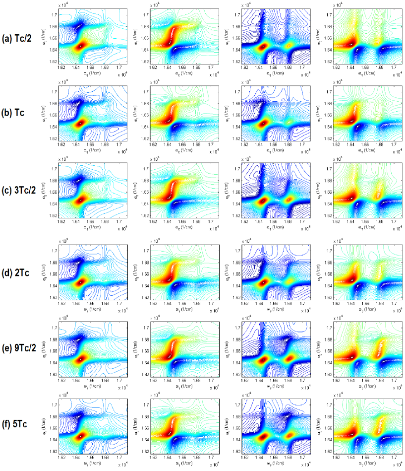
Figure 7: 2D-ES for coupled porphyrin homodimer with secular Redfield model. From left to right, we show the real and imaginary parts of the spectrum with $zzzz$ polarization setting (first and second columns), and with $zzxx$ setting (third and fourth columns). Each row represents a particular waiting time $T$, corresponding to (a) $T_{c}/2$, (b) $T_{c}$, (c) $3T_{c}/2$, (d) $2T_{c}$, (e) $9T_{c}/2$, (f) $5T_{c}$, where $T_{c}=47.5\,fs$ is the period for one Rabi oscillation between $|\alpha\rangle$ and $|\beta\rangle$. The colormap is such that red is associated with positive numbers, green with values about zero, and blue with negative numbers.

From the simulated spectra $\langle S(\omega_{\tau},T,\omega_{t})\rangle_{e_{1}e_{2}e_{3}e_{4}}$, the extraction of the terms $\langle S_{mn}(T)\rangle_{e_{1}e_{2}e_{3}e_{4}}$ is achieved with high fidelity (>99%) by a nonlinear optimization routine based on the simplex search method with bound constraints siam . The signals are fitted to a sum of four different resonances as in the isotropically averaged version of Eq. (32). The parameters $\omega_{mg}$, $\omega_{ng}$, $\Gamma$, and $\langle S_{mn}(T)\rangle_{e_{1}e_{2}e_{3}e_{4}}$ are reconstructed from 2D-ES with a grid spacing of $\Delta\omega_{\tau}=\Delta\omega_{t}=1\,cm^{-1}$ and a grid size of $1050\,cm^{-1}$ for every axis. We present the results of this calculation in Figure 8. Notice that the imaginary parts of the diagonal peaks are zero since no terms of the form $\chi_{\beta\alpha\alpha\beta}(T)=(\chi_{\alpha\beta\beta\alpha}(T))^{*}$are considered in the secular Redfield theory, and population transfer terms are purely real.

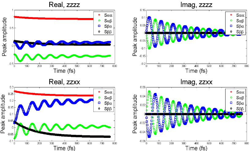
Figure 8: Traces of $\langle S_{mn}(T)\rangle_{e_{1}e_{2}e_{3}e_{4}}$ for $m,n\in\{\alpha,\beta\}$ and $(\boldsymbol{e}_{1},\boldsymbol{e}_{2},\boldsymbol{e}_{3},\boldsymbol{e}_{4})\in\{(\boldsymbol{z},\boldsymbol{z},\boldsymbol{z},\boldsymbol{z}),(\boldsymbol{z},\boldsymbol{z},\boldsymbol{x},\boldsymbol{x})\}$. (a) Real and (b) imaginary parts for the $zzzz$ configuration; (c) real and (d) imaginary parts for the $zzxx$ configuration. Each of the plots shows the evolution of the peak amplitudes $S_{\alpha\alpha}(T)$ (red crosses), $S_{\alpha\beta}(T)$ (green circles), $S_{\beta\alpha}(T)$ (blue squares), and $S_{\beta\beta}(T)$ (black diamonds).

Eq. (117) is solved at every waiting time $T\in[T_{c}/2,10T_{c}]$ yielding the roots $\xi=1.000,0.4059$ for every $T$, without variance after the fourth decimal digit, indicating its robustness for the inversion of $\phi$. The same exercise with Eq. (118) gives $\xi=-0.4059,0.4059$. These values of $\xi$ imply $\phi=90^{0},65^{0},65^{0},86.3i^{0}$, respectively. The last value can be discarded for it is not even a real number. The value of $\phi$ must be a root of both equations. Therefore, we can also discard $90^{0}$, since it is only solution of the first equation, but not of the second. The result $\phi=65^{0}$ follows unambiguously, as expected.

Finally, the terms $\langle S_{mn}(T)\rangle_{e_{1}e_{2}e_{3}e_{4}}$ and the angle $\phi$ allow for the evaluation of the elements of $\chi(T)$ which are extractable for the homodimer. Figure 9 shows that this reconstruction coincides with the analytical expressions presented in Table 4. The population decay terms $\chi_{\alpha\alpha\alpha\alpha}(T),\chi_{\beta\beta\beta\beta}(T)$ both start at 1 and reach 0 exponentially, the second faster than the first, since $|\beta\rangle$ is the excitonic state of higher energy. The population transfer terms $\chi_{\alpha\alpha\beta\beta}(T),\chi_{\beta\beta\alpha\alpha}(T)$ are complementary to the former ones, with the transfer from $|\beta\rangle$ to $|\alpha\rangle$ being faster for the same reasons just mentioned. The coherence term decays exponentially, with real and imaginary parts $\pi/2$ phase shifted one from another. The calculated timescale of this decay (hundreds of femtoseconds) is similar to the one inferred from the experiment reported by Lee and coworkers, where a superposition of excitons in the bacteriopheophytin and bacteriochlorophyll sites in the reaction center of purple bacteria is monitored indirectly through a two-color experiment HohjaiLee06082007 .

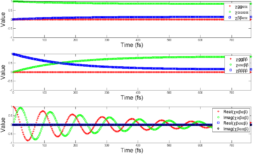
Figure 9: Extractable elements of $\chi(T)$ for homodimer. (a) Processes starting from $|\alpha\rangle\langle\alpha|$: $\chi_{gg\alpha\alpha}(T)$ (red crosses), $\chi_{\alpha\alpha\alpha\alpha}(T)$ (green circles), $\chi_{\beta\beta\alpha\alpha}(T)$ (blue squares). (b) Processes starting from $|\beta\rangle\langle\beta|$: $\chi_{gg\beta\beta}(T)$ (red crosses), $\chi_{\alpha\alpha\beta\beta}(T)$ (green circles), $\chi_{\beta\beta\beta\beta}$ (blue squares). (c) Processes indicating coherence transfer: $\Re\{\chi_{\alpha\beta\alpha\beta}(T)\}$ (red crosses), $\Im\{\chi_{\alpha\beta\alpha\beta}(T)\}$ (green circles), $\Re\{\chi_{\beta\alpha\alpha\beta}(T)\}$ (blue squares), $\Im\{\chi_{\beta\alpha\alpha\beta}(T)\}$ (black diamonds).

VI Discussion

In the present article, we have outlined a general theory for carrying out a QPT for a molecular dimer using the information contained in various frequency and polarization controlled 2D-ES. We started by providing the basic concepts of QPT, and operationally defined a QPT as a protocol to extract the process matrix $\chi(T)$, which in principle completely characterizes a quantum black box, in our case, the box being the single-exciton manifold of the dimer. After reviewing the model Hamiltonian as well as the transition dipole moments of an excitonic dimer, we adapted the QPT theory presented in our previous work, where the nonlinear polarization was analyzed in real time for single values of $\tau$ and $t$ times (see Eqs. (26), (27), and (28)) yuenzhou , to the more standard and visual Fourier transformed signal collected along several values of these interval times. The central result of this exercise was Eqs. (35), (36), (37), and (38), which from a purist stanpoint completes the QPT effort: The peaks in a heterodyne-detected 2D-ES can be expressed as linear combinations of elements of the process matrix $\chi(T)$. This information can be distilled by carrying out several experiments alternating the frequency components of the pulses as well as their polarization. By setting up a system of linear equations with this data, a linear algebraic routine yields the inversion of $\chi(T)$ for every waiting time $T$. In order to get a more intuitive picture of this procedure, the particular case of a homodimer was studied in detail. The degeneracies of this system yield a perpendicular set of transition dipole moments which considerably simplify the theory (see Fig. 5). It was shown that under isotropic average of the signal, no population to coherence processes or viceversa can be monitored, impeding a full QPT for the single-exciton manifold of this system. However, the partially achievable QPT is very simple, robust with respect to transition dipole moment parameters as long as they are not aligned or antialigned, and readily implemented without pulse shaping. The only requirement is the collection of two polarization controlled 2D-ES. Numerical examples with a model homodimer validated the presented theory.

The possibilities that QPT opens for the study of excited state dynamics in condensed molecular systems are as vast as the information acquired at the amplitude level of the evolving quantum state of the probed system. On the one hand, with the peaks in the 2D spectrum indicating a plethora of pathways in Liouville space, understanding of the dynamics is undoubtedly enhanced by the dissection of these peaks into processes described by the $\chi(T)$ matrix. On the other hand, a plethora of questions can be addressed with this information, for instance: Is a Markovian description accurate? AkihitoIshizaki10132009 ; ishizakijcp ; ChengEngel ; renger:9997 If not, what is the degree of non-Markovianity of the dynamics? breuernonmarkovian ; patricknonmarkovian If it is Markovian, is the secular Redfield equation appropriate or are non-secular processes important? ungar . Is there any degree of entanglement in the quantum states produced in the single exciton manifold upon photoexcitation? sarovar ; ishizakinjp What is the rate of decoherence of a quantum superposition between excitonic states? mancalspec ; olsinamancal ; abramaviciuslindblad ; hayesengel ; schlaujpcb

A few aspects have not been fully addressed with respect to the implementation of QPT of a molecular dimer. These issues will be carefully studied in future publications in collaboration with experimental groups. The role of static disorder in the eigenenergies of the system as well as in the distribution of the angle $\phi$ will necessarily yield an inhomogenously averaged signal from which the relevant information must be carefully extracted. We anticipate this feature to add another step of parameter fitting, but not change the results of our theory dramatically. Furthermore, we have ignored the possibility of resolving the vibronic structure accompanying each of the four resonances in the 2D-ES. If this were to happen, it might be wiser to take the approach of Cina and coworkers cinakilinhumble ; cinabiggs1 ; cinabiggs2 to consider the evolution of the nuclear wavepackets for a few modes strongly coupled to the system, and maybe regard the rest of the modes as a bosonic bath. This possibility would require an exponential increase of experimental resources resources , so either partial or compressed sensing approaches rabitz ; shabani would be necessary. Alternatively, by going back to the time-domain picture provided by the authors in their previous work yuenzhou , and applying novel concepts of QPT for initially correlated states kavancesar ; kavanpra ; kavanarxiv , a coarse grained and consistent tomographic protocol could be designed to address this problem. Finally, it might be worth considering additional nonlinear optical spectroscopic techniques such as considering the analysis of both rephasing and non-rephasing signals cheng ; readjpcb , transient grating ppv , pump probe khalil:362 , or phase cycling of multipulse induced fluorescence tekavec:214307 to investigate if they provide additional information for a more robust QPT.

Albeit this article not being exhaustive, we hope to have convinced the reader that the QPT approach follows the spirit of MDOS in a very natural way. By systematically studying excited state dynamics as a quantum black box, an intriguing perspective on MDOS emerges that allows the use of tools designed in the QIP community in order to study excited state dynamics of condensed molecular systems. These possibilities will be the subject of future studies.

VII Acknowledgments

We wish to acknowledge valuable discussions with Dr. Jacob Krich and Dr. Paul Peng on nonlinear spectroscopy, Seungwan Ryu on time-bandwidth issues, and Patrick Wen, Dylan Arias, Gabriela Schlau-Cohen, and Eleonora de Re for insights on experimental realizations of QPT. This work was funded by DARPA-QUBE as well as the Center for Excitonics.

APPENDIX: Derivation of Eqs. (6), (4), and (3)

Proof of Eq. (6).– Consider a system $S$ interacting with a bath $B$. The total density matrix of the composite object is $\rho_{total}$, whereas the reduced one for the system and the bath are $\rho$ and $\rho_{B}$, respectively. Suppose that the total initial state is a tensor product of the form:

$$\rho_{total}(0)=\rho(0)\otimes\rho_{B}(0).$$ (120)

Where $\rho_{B}(0)$ is assumed to be fixed at:

$$\rho_{B}(0)=\sum_{\beta}p_{\beta}|e_{\beta}\rangle\langle e_{\beta}|,$$ (121)

with $p_{\beta}\geq 0$, for every initial state $\rho(0)$ of the system.

At time $T$, the state of the composite object is simply a rotation of the initial state (it is a closed system):

$$\rho_{total}(T)=U(T)\rho_{total}(0)U^{+}(T).$$ (122)

Here, $U(T)=\mathcal{T}(e^{-i\int_{0}^{T}H_{total}(t^{\prime})dt^{\prime}})$ is the propagator for the entire object, where $\mathcal{T}$ is the time-ordering operator, and $H_{total}$ is given by:

$$H_{total}=H_{S}+H_{B}+H_{SB},$$ (123)

where $H_{S},H_{B},H_{SB}$ are terms in the Hamiltonian that depend only on $S$, on $B$, or on degrees of freedom of both, respectively. Taking the trace of Eq. (122) with respect to the states of $B$ yields $\rho(T)$:

$$\rho(T)=\sum_{\alpha\beta}E_{\alpha\beta}(T)\rho(0)E_{\alpha\beta}^{+}(T)$$ (124)

where:

$$E_{\alpha\beta}(T)=\sqrt{p_{\beta}}\langle e_{\alpha}|U(T)|e_{\beta}\rangle,$$ (125)

is a Kraus operator and Eq. (124) is often known as the operator sum representation Choi1975285 ; sudarshan . By identifying:

$$\chi_{abcd}(T)=\sum_{\alpha\beta}[E_{\alpha\beta}(t)]_{ac}[E_{\alpha\beta}^{+}(t)]_{db},$$ (126)

we have shown the equivalence between Eq. (124) and (6).

$\Box$

Proof of Eq. (3).–As explained in Section II and in the previous proof, Eq. (6) holds for any proper or improper state $\rho(0)$ in the Liouville space of the system. With this in mind, Eq. (3) is straightforward to prove. We want to enforce that Eq. (6) preserves trace throughout the evolution in time $T$. If $\rho(0)=|k\rangle\langle l|$, then it must be that $Tr(\rho(T))=Tr(\rho(0))=\delta_{kl}$. Writing the elements of the initial density matrix as $\rho_{cd}(0)=\delta_{ck}\delta_{dl}$, we immediately obtain the condition we want to prove:

$$Tr(\rho(T)) = \sum_{a}\delta_{ab}\sum_{cd}\chi_{abcd}\delta_{ck}\delta_{dl},$$

$$\delta_{kl} = \chi_{aakl}.$$ (127)

$\Box$

Proof of Eq. (4).– Again, we exploit the fact that Eq. (6) is true for any $\rho(0)$.

First, we consider a population as the initial state, i.e. $\rho(0)=|k\rangle\langle k|$ for any $k$. Note that $\rho(0)$ is a proper density matrix, and hence Hermitian. Then,

$$\rho_{ab}(T) = \sum_{cd}\chi_{abcd}(T)\delta_{ck}\delta_{dk}$$ (128)

$$= \chi_{abkk}(T),$$

$$\rho_{ba}(T) = \sum_{dc}\chi_{bacd}(T)\delta_{ck}\delta_{dk}$$ (129)

$$= \chi_{bakk}(T).$$

Since $\chi(T)$ maps proper density matrices to proper density matrices, $\rho(T)$ must also be Hermitian, i.e. $\rho_{ba}(T)=\rho_{ab}^{*}(T)$. It follows from Eqs. (128) and (129) that for any $a,b,k$:

$$\chi_{bakk}(T)=\chi_{abkk}^{*}(T).$$ (130)

This proves Eq. (4) for the case $c=d$. Next, we consider initial proper states of the form $\rho(0)=\frac{1}{2}(|k\rangle\langle k|+|k\rangle\langle l|+|l\rangle\langle k|+|l\rangle\langle l|)$. By repeating the exercise above, we get:

$$\frac{1}{2}(\chi_{bakk}(T)+\chi_{bakl}(T)+\chi_{balk}(T)+\chi_{ball}(T))=\frac{1}{2}(\chi_{abkk}(T)+\chi_{abkl}(T)+\chi_{ablk}(T)+\chi_{abll}(T))^{*}$$ (131)

Substituting the result Eq. (130) into Eq. (131) yields:

$$\chi_{bakl}(T)+\chi_{balk}(T)=\chi_{abkl}^{*}(T)+\chi_{ablk}^{*}(T)$$ (132)

This result almost proves Eq. (4) for the case $c\neq d$. In order to complete the proof, we analyze another class of initial proper states $\rho(0)=\frac{1}{2}(|k\rangle\langle k|+i|k\rangle\langle l|-i|l\rangle\langle k|+|l\rangle\langle l|)$. The result from the same manipulations is that:

$$i\chi_{bakl}(T)-i\chi_{balk}(T)=-i\chi_{abkl}^{*}(T)+i\chi_{ablk}^{*}(T)$$ (133)

Comparing Eqs. (131) and (132) yields:

$$\chi_{bakl}(T) = \chi_{ablk}^{*}(T)$$

$$\chi_{balk}(T) = \chi_{abkl}^{*}(T)$$ (134)

for any $a,b,k,l$. Eqs. (130) and (134) together yield Eq. (4).

References

- [1] S. Mukamel. Principles of Nonlinear Optical Spectroscopy. Oxford University Press, 1995.
- [2] M. Cho. Two Dimensional Optical Spectroscopy. CRC Press, 2009.
- [3] Minhaeng Cho. Coherent two-dimensional optical spectroscopy. Chem. Rev., 108:1331–1418, 2008.
- [4] S. Mukamel, Y. Tanimura, and P. Hamm. Coherent multidimensional optical spectroscopy. Acc. Chem. Res., 42:1207–1209, 2009.
- [5] D. M. Jonas. Two-dimensional femtosecond spectroscopy. Ann. Rev. Phys. Chem., 54:425–463, 2003.
- [6] S. Mukamel, D. Abramavicius, L. Yang, W. Zhuang, I. V. Schweigert, and D. V. Voronine. Coherent multidimensional optical probes for electron correlations and exciton dynamics: From nmr to x-rays. Acc. Chem. Res., 42(4):553–562, 2009.
- [7] E. Harel, A. F. Fidler, and G. S. Engel. Real-time mapping of electronic structure with single-shot two-dimensional electronic spectroscopy. Proc. Natl. Acad. Sci. USA, 107(38):16444–16447, 2010.
- [8] Thomas Steffen and Koos Duppen. Femtosecond two-dimensional spectroscopy of molecular motion in liquids. Phys. Rev. Lett., 76(8):1224–1227, 1996.
- [9] M.l D. Fayer, D. E. Moilanen, D. Wong, D. E. Rosenfeld, E. E. Fenn, and S. Park. Water Dynamics in Salt Solutions Studied with Ultrafast Two-Dimensional Infrared (2D IR) Vibrational Echo Spectroscopy. Acc. Chem. Res., 42(9, Sp. Iss. SI):1210–1219, 2009.
- [10] S. A. Miller and A. M. Moran. Nonlinear optical detection of electron transfer adiabaticity in metal polypyridyl complexes. J. Phys. Chem. A, 114(5):2117–2126, 2010.
- [11] M. Khalil, N. Demirdöven, and A. Tokmakoff. Vibrational coherence transfer characterized with fourier-transform 2d ir spectroscopy. J. Chem. Phys., 121:362–373, 2004.
- [12] M. Khalil, N. Demirdoven, and A. Tokmakoff. Coherent 2D IR spectroscopy: Molecular structure and dynamics in solution. J. Phys. Chem. A, 107(27):5258–5279, 2003.
- [13] C. R. Baiz, P. L. McRobbie, J. M. Anna, E. Geva, and K. J. Kubarych. Two-dimensional infrared spectroscopy of metal carbonyls. Acc. Chem. Res., 42(9):1395–404, 2009.
- [14] Z. Bihary, M. Karavitis, and V. A. Apkarian. Onset of decoherence: Six-wave mixing measurements of vibrational decoherence on the excited electronic state of i[sub 2] in solid argon. J. Chem. Phys., 120(17):8144–8156, 2004.
- [15] M. Guhr and N. Schwentner. Coherent phonon dynamics: Br-2 in solid Ar. Phys. Chem. Chem. Phys., 7(5):760–767, 2005.
- [16] Katsuyoshi Ikeda and Kohei Uosaki. Coherent phonon dynamics in single-walled carbon nanotubes studied by time-frequency two-dimensional coherent anti-stokes raman scattering spectroscopy. Nano Lett., 9(4):1378–1381, 2009.
- [17] H. S. Chung, Z. Ganim, K. C. Jones, and A. Tokmakoff. Transient 2D IR spectroscopy of ubiquitin unfolding dynamics. Proc. Natl. Acad. Sci. USA, 104(36), 2007.
- [18] G. Panitchayangkoon, D. Hayes, K. A. Fransted, J. R. Caram, E. Harel, J. Wen, R. E. Blankenship, and G. S. Engel. Long-lived quantum coherence in photosynthetic complexes at physiological temperature. Proc. Natl. Acad. Sci. USA, 107(29):12766–12770, 2010.
- [19] G. S. Engel, T. R. Calhoun, E. L. Read, T. K. Ahn, T. Mancal, Y. C. Cheng, R. E. Blankenship, and G. R. Fleming. Evidence for wavelike energy transfer through quantum coherence in photosynthetic systems. Nature, 446:782–786, 2007.
- [20] E. Collini, C. Y. Wong, K. E. Wilk, P. M. G. Curmi, P. Brumer, and G. D. Scholes. Coherently wired light-harvesting in photosynthetic marine algae at ambient temperature. Nature, 463:644–U69, 2010.
- [21] J. M. Womick and A. M. Moran. Exciton Coherence and Energy Transport in the Light-Harvesting Dimers of Allophycocyanin. J. Phys. Chem. B, 113:15747–15759, 2009.
- [22] N. Christensson, F. Milota, A. Nemeth, J. Sperling, H. F. Kauffmann, T. Pullerits, and J. Hauer. Two-dimensional electronic spectroscopy of beta-carotene. J. Phys. Chem. B, 113(51):16409–16419, 2009.
- [23] F. Milota, J. Sperling, A. Nemeth, T. Mancal, and H. F. Kauffmann. Two-dimensional electronic spectroscopy of molecular excitons. Acc. Chem. Res., 42(9):1364–1374, 2009.
- [24] Elisabetta Collini and Gregory D. Scholes. Coherent intrachain energy migration in a conjugated polymer at room temperature. Science, 323:369–373, 2009.
- [25] E. Collini and G. D. Scholes. Electronic and vibrational coherences in resonance energy transfer along meh-ppv chains at room temperature. The Journal of Physical Chemistry A, 113(16):4223–4241, 2009.
- [26] K. W. Stone, K. Gundogdu, D. B. Turner, X. Li, S. T. Cundiff, and K. A. Nelson. Two-Quantum 2D FT Electronic Spectroscopy of Biexcitons in GaAs Quantum Wells. Science, 324:1169–1173, 2009.
- [27] D. B. Turner and K. A. Nelson. Coherent measurements of high-order electronic correlations in quantum wells. Nature, 466(7310):1089–1092, 2010.
- [28] D.B. Turner, K.W. Stone, K. Gundogdu, and K.A. Nelson. Three-dimensional electronic spectroscopy of excitons in gaas quantum wells. J. Chem. Phys., 131(14):144510, 2009.
- [29] Cathy Y. Wong and Gregory D. Scholes. Using two-dimensional photon echo spectroscopy to probe the fine structure of the ground state biexciton of cdse nanocrystals. J. Lumin., in Press:–, 2010.
- [30] M. A. Nielsen and Chuang I. L. Quantum Computation and Quantum Information. Cambridge University Press, 2000.
- [31] I. L. Chuang and M. A. Nielsen. Prescription for experimental determination of the dynamics of a quantum black box. J. Mod. Opt., 44:2455–2467, 1997.
- [32] M. Mohseni and D. A. Lidar. Direct characterization of quantum dynamics. Phys. Rev. Lett., 97:170501, 2006.
- [33] M. Mohseni, A. T. Rezakhani, and D. A. Lidar. Quantum-process tomography: Resource analysis of different strategies. Phys. Rev. A, 77:032322, 2008.
- [34] J. Yuen-Zhou, M. Mohseni, and A. Aspuru-Guzik. Quantum Process Tomography of Multichromophoric Systems via Ultrafast Spectroscopy. ArXiv e-prints, 2010.
- [35] M.D. Choi. Completely positive linear maps on complex matrices. Linear Algebra Appl., 10(3):285 – 290, 1975.
- [36] E. C. G. Sudarshan, P. M. Mathews, and Jayaseetha Rau. Stochastic dynamics of quantum-mechanical systems. Phys. Rev., 121(3):920–924, 1961.
- [37] U. Leonhardt. Quantum-state tomography and discrete wigner function. Phys. Rev. Lett., 74:4101–4105, 1995.
- [38] T. J. Dunn, I. A. Walmsley, and S. Mukamel. Experimental determination of the quantum-mechanical state of a molecular vibrational mode using fluorescence tomography. Phys. Rev. Lett., 74:884–887, 1995.
- [39] C. Leichtle, W. P. Schleich, I. Sh. Averbukh, and M. Shapiro. Quantum state holography. Phys. Rev. Lett., 80:1418–1421, 1998.
- [40] T. S. Humble and J. A. Cina. Molecular state reconstruction by nonlinear wave packet interferometry. Phys. Rev. Lett., 93:060402, 2004.
- [41] J. A. Cina. Nonlinear wavepacket interferometry for polyatomic molecules. J. Chem. Phys., 113:9488–9496, 2000.
- [42] Y. S. Weinstein, T. F. Havel, J. Emerson, N. Boulant, M. Saraceno, S. Lloyd, and D. G. Cory. Quantum process tomography of the quantum fourier transform. J. Chem. Phys., 121:6117–6133, 2004.
- [43] A. M. Childs, I. L. Chuang, and D. W. Leung. Realization of quantum process tomography in nmr. Phys. Rev. A, 64:012314, 2001.
- [44] H. Kampermann and W. S. Veeman. Characterization of quantum algorithms by quantum process tomography using quadrupolar spins in solid-state nuclear magnetic resonance. J. Chem. Phys., 122:214108, 2005.
- [45] M. Riebe, K. Kim, P. Schindler, T. Monz, P. O. Schmidt, T. K. Körber, W. Hänsel, H. Häffner, C. F. Roos, and R. Blatt. Process tomography of ion trap quantum gates. Phys. Rev. Lett., 97:220407, 2006.
- [46] J. B. Altepeter, D. Branning, E. Jeffrey, T. C. Wei, P. G. Kwiat, R. T. Thew, J. L. O’Brien, M. A. Nielsen, and A. G. White. Ancilla-assisted quantum process tomography. Phys. Rev. Lett., 90:193601, 2003.
- [47] M. W. Mitchell, C. W. Ellenor, S. Schneider, and A. M. Steinberg. Diagnosis, prescription, and prognosis of a bell-state filter by quantum process tomography. Phys. Rev. Lett., 91(12):120402, 2003.
- [48] M. Howard, J. Twamley, C. Wittmann, T. Gaebel, F. Jelezko, and J. Wrachtrup. Quantum process tomography and linblad estimation of a solid-state qubit. New J. Phys., 8:33, 2006.
- [49] S. H. Myrskog, J. K. Fox, M. W. Mitchell, and A. M. Steinberg. Quantum process tomography on vibrational states of atoms in an optical lattice. Phys. Rev. A, 72:013615, 2005.
- [50] R. C. Bialczak, M. Ansmann, M. Hofheinz, E. Lucero, M. Neeley, A. D. O’Connell, D. Sank, H. Wang, J. Wenner, M. Steffen, A. N. Cleland, and J. M. Martinis. Quantum process tomography of a universal entangling gate implemented with Josephson phase qubits. Nat. Phys., 6(6):409–413, 2010.
- [51] M. Yang and G.R. Fleming. Two-color three-pulse photon echoes as a probe of electronic coupling in molecular complexes. J. Chem. Phys., 110(6):2983–2990, 1999.
- [52] Kjellberg P. and Pullerits T. Three-pulse photon echo of an excitonic dimer modeled via redfield theory. J. Chem. Phys., 124(2):024106, 2006.
- [53] Seidner L., Stock G., and Domcke W. Nonperturbative approach to femtosecond spectroscopy: General theory and application to multidimensional nonadiabatic photoisomerization processes. J. Chem. Phys., 103(10):3998–4011, 1995.
- [54] P. Kjellberg, B. Brüggemann, and T. Pullerits. Two-dimensional electronic spectroscopy of an excitonically coupled dimer. Phys. Rev. B, 74(2):024303, 2006.
- [55] M.F. Gelin, Egorova D., and Domcke W. Efficient method for the calculation of time- and frequency-resolved four-wave mixing signals and its application to photon-echo spectroscopy. J. Chem. Phys., 123(16):164112, 2005.
- [56] I. D. Abella, N. A. Kurnit, and S. R. Hartmann. Photon echoes. Phys. Rev., 141(1):391–406, 1966.
- [57] N. A. Kurnit, I. D. Abella, and S. R. Hartmann. Observation of a photon echo. Phys. Rev. Lett., 13(19):567–568, 1964.
- [58] M. Cho, T. Brixner, I. Stiopkin, H. Vaswani, and Fleming G. Two-dimensional electronic spectroscopy of molecular complexes. J. Chin. Chem. Soc., 53:15–24, 2006.
- [59] Y. C. Cheng and G. R. Fleming. Coherence quantum beats in two-dimensional electronic spectroscopy. J. Phys. Chem. A, 112:4254–4260, 2008.
- [60] M.F. Gelin and D.S. Kosov. Doorway-window description of sequential three-pulse photon echo signals. Chem. Phys., 347(1-3):177 – 184, 2008. Ultrafast Photoinduced Processes in Polyatomic Molecules - Electronic Structure, Dynamics and Spectroscopy.
- [61] D.P. Craig and T. Thirunamachandran. Molecular quantum electrodynamics: An introduction to radiation molecule interactions. Dover Publications, 1998.
- [62] D. V. Voronine, D. Abramavicius, and Mukamel S. Manipulating multidimensional electronic spectra of excitons by polarization pulse shaping. J. Chem. Phys., 126(4):044508, 2007.
- [63] D. Abramavicius, V. Butkus, J. Bujokas, and Valkunas L. Manipulation of two-dimensional spectra of excitonically coupled molecules by narrow-bandwidth laser pulses. Chem. Phys., 372(1-3):22 – 32, 2010.
- [64] S. Woutersen and P. Hamm. Structure determination of trialanine in water using polarization sensitive two-dimensional vibrational spectroscopy. J. Phys. Chem. B, 104(47):11316–11320, 2000.
- [65] F. Perakis and P. Hamm. Two-dimensional infrared spectroscopy of supercooled water. J. Phys. Chem. B, 0(0), 0.
- [66] D.B. Strasfeld, C.T. Middleton, and M.T. Zanni. Mode selectivity with polarization shaping in the mid-ir. New J. Phys., 11(10):105046, 2009.
- [67] J. M. Womick, S. A. Miller, and A. M. Moran. Correlated exciton fluctuations in cylindrical molecular aggregates. J. Phys. Chem. B, 113(19):6630–6639, 2009.
- [68] J. M. Womick, S. A. Miller, and A. M. Moran. Probing the dynamics of intraband electronic coherences in cylindrical molecular aggregates. J. Phys. Chem. A, 113(24):6587–6598, 2009.
- [69] G. S. Schlau-Cohen, T. R. Calhoun, N. S. Ginsberg, M. Ballottari, R. Bassi, and G. R. Fleming. Spectroscopic elucidation of uncoupled transition energies in the major photosynthetic light-harvesting complex, LHCII. Proc. Natl. Acad. Sci. USA, 107(30):13276–13281, 2010.
- [70] W. Cheney and D. Kincaid. Numerical mathematics and computing. Thomson-Brooks/Cole, sixth edition, 2008.
- [71] G.A. Lott, A. Perdomo-Ortiz, J. K. Utterback, A. Aspuru-Guzik, and A. H. Marcus. Structure of self-assembled porphyrin dimers in phospholipid membranes by fluorescence-detected 2d phase-modulation electronic coherence spectroscopy. Submitted, 2010.
- [72] A. V. Pisliakov, T. Mančal, and G. R. Fleming. Two-dimensional optical three-pulse photon echo spectroscopy. ii. signatures of coherent electronic motion and exciton population transfer in dimer two-dimensional spectra. J. Chem. Phys., 124:234505, 2006.
- [73] J. C. Lagarias, J. A. Reeds, M. H. Wright, and P. E. Wright. Convergence properties of the Nelder-Mead simplex method in low dimensions. SIAM J. Optimiz., 9(1):112–147, 1998.
- [74] H. Lee, Y. C. Cheng, and G. R. Fleming. Coherence Dynamics in Photosynthesis: Protein Protection of Excitonic Coherence. Science, 316:1462–1465, 2007.
- [75] Akihito Ishizaki and Graham R. Fleming. Theoretical examination of quantum coherence in a photosynthetic system at physiological temperature. Proc. Natl. Acad. Sci., 106:17255–17260, 2009.
- [76] Ishizaki A. and Fleming G. R. On the adequacy of the redfield equation and related approaches to the study of quantum dynamics in electronic energy transfer. J. Chem. Phys., 130(23):234110, 2009.
- [77] Yuan-Chung Cheng, Gregory S. Engel, and Graham R. Fleming. Elucidation of population and coherence dynamics using cross-peaks in two-dimensional electronic spectroscopy. Chemical Physics, 341(1-3):285 – 295, 2007. Ultrafast Dynamics of Molecules in the Condensed Phase: Photon Echoes and Coupled Excitations - A Tribute to Douwe A. Wiersma.
- [78] T. Renger and R.A. Marcus. On the relation of protein dynamics and exciton relaxation in pigment–protein complexes: An estimation of the spectral density and a theory for the calculation of optical spectra. J. Chem. Phys., 116(22):9997–10019, 2002.
- [79] Heinz-Peter Breuer, Elsi-Mari Laine, and Jyrki Piilo. Measure for the degree of non-markovian behavior of quantum processes in open systems. Phys. Rev. Lett., 103(21):210401, 2009.
- [80] P. Rebentrost and A. Aspuru-Guzik. Exciton-phonon information flow in the energy transfer process of photosynthetic complexes. ArXiv e-prints, 2010.
- [81] L. W. Ungar and J. A. Cina. The relaxation dynamics and short-time optical response of a multimode open system. J. Phys. Chem. A, 102(38):7382–7392, 1998.
- [82] Fleming G.R. Sarovar M., Ishizaki A. and Whaley K.B. Quantum entanglement in photosynthetic light-harvesting complexes. Nature Physics, 6:462, 2010.
- [83] Ishizaki A. and Fleming G.R. Quantum superpositions in photosynthetic light harvesting: delocalization and entanglement. New J. Phys., 12(5):055004, 2010.
- [84] T. Mancal, L. Valkunas, E. L. Rea, G. S. Engel, T. R. Calhoun, and G. R. Fleming. Electronic coherence transfer in photosynthetic complexes and its signatures in optical spectroscopy. Spectrosc. Int. J., 22(2-3):199–211, 2008.
- [85] J. Olsina and T. Mancal. Electronic coherence dephasing in excitonic molecular complexes: Role of Markov and secular approximations. J. Mol. Model., 16(11):1765–1778, 2010.
- [86] D. Abramavicius and S. Mukamel. Quantum oscillatory exciton migration in photosynthetic reaction centers. J. Chem. Phys., 133(6):064510, 2010.
- [87] D. Hayes, G. Panitchayangkoon, K. A. Fransted, J. R. Caram, J. Wen, K. F. Freed, and G.S. Engel. Dynamics of electronic dephasing in the fenna matthews olson complex. New Journal of Physics, 12(6):065042, 2010.
- [88] G. S. Schlau-Cohen, T. R. Calhoun, N. S. Ginsberg, E. L. Read, M. Ballottari, R. Bassi, R. van Grondelle, and G. R. Fleming. Pathways of energy flow in lhcii from two-dimensional electronic spectroscopy. J. Phys. Chem. B, 113(46):15352–15363, 2009.
- [89] J. A. Cina, D. S. Kilin, and T. S. Humble. Wavepacket interferometry for short-time electronic energy transfer: Multidimensional optical spectroscopy in the time domain. J. Chem. Phys., 118:46–61, 2003.
- [90] J. D. Biggs and J. A. Cina. Using wave-packet interferometry to monitor the external vibrational control of electronic excitation transfer. J. Chem. Phys., 131:224101, 2009.
- [91] J. D. Biggs and J. A. Cina. Calculations of nonlinear wave-packet interferometry signals in the pump-probe limit as tests for vibrational control over electronic excitation transfer. J. Chem. Phys., 131:224302, 2009.
- [92] M. P. A. Branderhorst, J. Nunn, I. A. Walmsley, and R. L. Kosut. Simplified quantum process tomography. New J. Phys., 11:115010, 2009.
- [93] A. Shabani, M. Mohseni, S. Lloyd, R. L. Kosut, and H. Rabitz. Efficient estimation of nearly sparse many-body quantum hamiltonians. ArXiv e-prints, 2010.
- [94] A. M. Kuah, K. Modi, C. A. Rodríguez-Rosario, and E. C. G. Sudarshan. How state preparation can affect a quantum experiment: Quantum process tomography for open systems. Phys. Rev. A, 76(4):042113, 2007.
- [95] K. Modi and E. C. G. Sudarshan. Role of preparation in quantum process tomography. Phys. Rev. A, 81(5):052119, 2010.
- [96] K. Modi. Non-Markovian memory in quantum process tomography and a preparation independent map. ArXiv e-prints, 2010.
- [97] E. L.. Read, G. S. Schlau-Cohen, G. S. Engel, T. Georgiou, M. Z. Papiz, and G. R. Fleming. Pigment organization and energy level structure in light-harvesting complex 4: Insights from two-dimensional electronic spectroscopy. J. Phys. Chem. B, 113(18):6495–6504, 2009.
- [98] P. F. Tekavec, G. A. Lott, and A. H. Marcus. Fluorescence-detected two-dimensional electronic coherence spectroscopy by acousto-optic phase modulation. J. Chem. Phys., 127:214307, 2007.
- [99] S. M. Gallagher Faeder and D. M. Jonas. Two-dimensional electronic correlation and relaxation spectra: Theory and model calculations. J. Phys. Chem. A, 103(49):10489–10505, 1999.
- [100] P. Rebentrost, S. Shim, J. Yuen-Zhou, and A. Aspuru-Guzik. Characterization and quantification of the role of coherence in ultrafast quantum biological experiments using quantum master equations, atomistic simulations, and quantum process tomography. ArXiv e-prints, 2010.