Matched Filtering from Limited Frequency Samples

Abstract

In this paper, we study a simple correlation-based strategy for estimating the unknown delay and amplitude of a signal based on a small number of noisy, randomly chosen frequency-domain samples. We model the output of this “compressive matched filter” as a random process whose mean equals the scaled, shifted autocorrelation function of the template signal. Using tools from the theory of empirical processes, we prove that the expected maximum deviation of this process from its mean decreases sharply as the number of measurements increases, and we also derive a probabilistic tail bound on the maximum deviation. Putting all of this together, we bound the minimum number of measurements required to guarantee that the empirical maximum of this random process occurs sufficiently close to the true peak of its mean function. We conclude that for broad classes of signals, this compressive matched filter will successfully estimate the unknown delay (with high probability, and within a prescribed tolerance) using a number of random frequency-domain samples that scales inversely with the signal-to-noise ratio and only logarithmically in the observation bandwidth and the possible range of delays.

1 Introduction

1.1 Random Sampling and Compressive Signal Processing

Over the last few decades, the development of cheap, flexible, and powerful digital signal processing (DSP) architectures has enabled the acquisition and analysis of increasingly rich data sets. One of the key principles behind the DSP revolution is the fundamental work by Nyquist, Whittaker, and Shannon in characterizing the minimum number of discrete-time samples required to fully capture the information in a bandlimited continuous-time signal. Unfortunately, many real-world signals of interest may have very high bandwidth, which can severely complicate the practical task of sampling a signal at its Nyquist rate [21, 35].

The recently developed theory of Compressive Sensing (CS) [5, 9] suggests that if a signal is structured, then we can acquire it by taking samples well below its Nyquist rate. CS relies on two fundamental principles: first, that many signals have much lower complexity than is suggested by their bandwidth (typically this is embodied in a sparse representation for the signal within some basis), and second, that such signals may safely be sampled below their Nyquist rate if the traditional uniform time-domain sampling procedure is replaced with a generalized linear measurement operator (typically this operator contains some degree of randomness).

The CS theory has benefited from several powerful and elegant tools for probabilistic analysis relating to the theory of empirical processes. The essential condition (the restricted isometry property [4]) that guarantees sparse recovery from observations through a random matrix can be recast as a bound on a random process — this formulation, first put forth in [34], is particularly useful when the compressive measurement system is structured [35, 28, 32, 33, 30]. In these works, the Dudley inequality [12], a classical tool which relates the supremum of a random process to the geometry of its index set, is used to bound the expected supremum of the process, and strong tail bounds are established that control the deviation from the average behavior. To date, almost all of the work along these lines has focused on providing guarantees for signal recovery from compressive measurements.

There are many applications, however, where we are not interested in a full-scale recovery of a signal. Instead, we may wish only to estimate some key parameters (or “features”) in order to solve an inference problem that does not demand full knowledge of the signal. It has been demonstrated that random measurements can again be very useful in such settings. Just as certain low-complexity signals can be fully recovered from random measurements, certain low-complexity questions can be answered about (possibly arbitrary) signals directly from random measurements without first recovering the signal. Some initial steps in this direction have been concerned with compressive detection, classification, estimation, and filtering [16, 11, 17, 7, 6]. Compared to alternative techniques that base their inference on a full set of Nyquist samples, compressive inference techniques can show slightly diminished accuracy because fewer statistics are measured concerning the signal. In exchange, the acquisition hardware can potentially be much simpler and consume less power. In addition, we maintain the ability to adapt to future information we may learn the problem at hand; from a single set of random measurements, a number of different inference problems may be solved concerning a number of possible candidate signals.

In this paper, we study the problem of matched filtering (i.e., estimating the unknown delay and amplitude of a known template signal) from the compressive viewpoint. In particular, we derive strong bounds on the performance of a compressive matched filter by bringing in some of the same probabilistic tools that have been so fruitful in CS recovery analysis. To do this, we show that the compressive matched filtering problem can be reduced to controlling the supremum of a certain random process, which we approach through a specialized version of the Dudley inequality.

1.2 Matched Filtering from Limited Frequency Samples

1.2.1 The Compressive Matched Filter

The problem that we consider is formally stated as follows. Suppose we make observations of the continuous-time signal $A\cdot s_{0}(t-\tau_{0})$, where $s_{0}(t)$ is a known signal template, $\tau_{0}\in T\subset\mathbb{R}$ is the unknown delay (the time-of-arrival), and $A\in\mathbb{R}$ or $\mathbb{C}$ is the unknown amplitude. Given these observations, we would like to estimate $\tau_{0}$ and $A$.

The optimal solution to this problem is given by the matched filter. All shifts of the known template $s_{0}(t)$ are correlated against the incoming signal, and the estimated time-of-arrival is the shift that yields the maximum correlation. The matched filter is typically implemented in one of two ways: either with a specialized analog circuit that performs the correlation and then detects the peaks, or by sampling the signal and calculating the correlation function digitally. The advantage of the digital approach is the flexibility it offers; we can perform matched filtering against many different waveforms from the same set of samples, in case $s_{0}(t)$ is not known in advance (but belongs to a collection of candidates). If the signal $s_{0}(t)$ is concentrated in time, the sampling rate must be commensurately high to accurately estimate $\tau_{0}$. Applications such as high-frequency radar or ultra-wideband communications can require sampling rates of hundred of millions, or even billions, of samples per second. Taking and processing samples at these kinds of rates is costly in terms of hardware complexity and power consumption.

Working from compressed samples gives us a more elegant solution. In this paper we analyze a simple correlation-based estimator that operates using a small number $m$ of noisy samples of spectrum of the received signal, with locations that are drawn randomly from a uniform distribution on some interval $\Omega$ in the frequency domain. In one of our main results (Corollary 6), we prove that for broad classes of signals, this compressive matched filter will successfully estimate $\tau_{0}$ (with high probability, and within a prescribed tolerance) using a number of random frequency-domain samples that scales inversely with the signal-to-noise ratio and only logarithmically in the observation bandwidth $|\Omega|$ and the possible range of delays $|T|$. Our results help validate the use of compressive measurements for capturing important signal information. This acquisition scheme also offers us flexibility in that it depends only on very broad characteristics of the signal; it is universally effective for all $s_{0}(t)$ which are spread out over the band $\Omega$.

We note that the use of randomized measurements in the frequency domain is not unprecedented. One of the original motivating problems for CS, for example, came from magnetic resonance imaging (MRI), where the goal is to reconstruct an image from a partial set of Fourier coefficients [5, 25]. Randomized frequency-domain measurements are also standard in CS problems where the signal to be recovered is sparse in the time domain [5, 34], and of course, in the compressive matched filter problem, the unknown signal delay is manifested in the time domain. In hardware, the requisite spectral samples for the compressive matched filter could be acquired by correlating the incoming signal with a bank of oscillators tuned to random frequencies, or by following a Fourier transforming device (such as a SAW processor [18]) with a random sampler. Although the analysis in our paper is limited to one-dimensional signals, one could also envision formulating the matched filtering problem for two-dimensional images, and random samples of a two-dimensional spectrum could be acquired by combining the Fourier transforming property of a lens with a random sampler.

1.2.2 Analytical Framework and Summary of Main Results

In this paper, we develop an analytical framework for studying the compressive matched filter based on tools from probability theory and empirical processes. To help build intuition, in Sections 2.1 through 2.4 we first study the problem fully in the case of noiseless measurements. In Section 2.5 we then extend all of our analysis in parallel fashion to account for measurement noise. Section 4 and several appendices provide supporting proofs for all of our main results.

For both the noiseless and noisy problem formulations, we begin by showing that the output of the correlation-based estimator can be modeled as a random process whose mean equals the scaled, shifted autocorrelation function of the template signal. Noting that the scaled, shifted autocorrelation function of the template signal (the mean of this random process) peaks at $\tau_{0}$, we estimate $\tau_{0}$ by finding the empirical maximum of the random process, and we give guarantees about the accuracy of this estimate by showing that the random process does not vary too much from its mean. Given the estimate of the delay, an estimate of the amplitude $A$ follows easily via least-squares, just as with the standard matched filer.

We approach the analysis as follows. In Theorems 1 and 4, we adapt the proof of the Dudley inequality to show that the expected maximum deviation of this random process from its mean decreases sharply as the number of measurements increases. A bit more formally, Theorem 1 states that in the noiseless case, the expected maximum deviation of this process from its mean decreases roughly like $m^{-1/2}$ (normalized by the peak value of the mean function). Theorem 4 quantifies the amount of additional deviation one would expect based on noise in the observations. In Theorems 2 and 5, we then derive a probabilistic tail bound on the maximum deviation of this process from its mean. Specifically, Theorem 2 guarantees that with high probability the noiseless process stays uniformly close to its mean, and Theorem 5 guarantees that with high probability the maximum additional deviation caused by noise is also bounded. Finally, in Corollaries 3 and 6, we pull these results together to establish bounds on the number of measurements required to guarantee that the empirical maximum of this random process occurs sufficiently close to the true peak of its mean function. Specifically, Corollary 3 ensures in the noiseless case that when the template signal has an autocorrelation function with a single prominent peak, no values of $\tau$ far from $\tau_{0}$ can yield an estimate close to the true peak. Corollary 6 extends this result to account for noise and leads to the central result: the compressive matched filter will successfully estimate $\tau_{0}$ from $m$ random frequency-domain samples (with high probability, and within a prescribed tolerance) as long as $m$ scales inversely with the signal-to-noise ratio and logarithmically in the observation bandwidth $|\Omega|$ and the possible range of delays $|T|$.

All of our bounds depend on the degree to which the template signal $s_{0}$ is concentrated in the frequency domain. As might be expected given the uniform random sampling strategy on $\Omega$, signals whose spectrum is relatively flat across $\Omega$ will require the fewest measurements, while signals with highly peaked spectra will require the most. These issues are carefully quantified and discussed in detail throughout Section 2.

1.2.3 Exchanging Time and Frequency

It is important to point out that the roles of time and frequency are completely interchangeable in our analysis. All of our results from Section 2 can therefore be adapted to the “dual” problem of estimating the unknown carrier frequency of a modulated signal given a small number of time-domain samples of that signal; the time domain becomes our observation domain, and the frequency domain becomes the domain in which we wish to determine the unknown shift of the known template signal. For the sake of space, we do not restate all of our results in this context, although the conclusion is clear: a compressive matched filter can successfully estimate an unknown modulation frequency $\omega_{0}$ from $m$ random time-domain samples (with high probability, and within a prescribed tolerance) as long as $m$ scales inversely with the signal-to-noise ratio and logarithmically in the observation duration $|T|$ and the possible range of carrier frequencies $|\Omega|$. (A Nyquist-based approach, in contrast, would require a sampling rate linearly proportional to $|\Omega|$ but could tolerate somewhat lower signal-to-noise ratios.) The bounds will also depend — in this case — on the degree to which the template signal is concentrated in the time domain. Signals whose envelope is relatively flat across $T$ will require the fewest measurements, while signals with highly peaked envelopes will require the most.

While we do not discuss this problem further in full generality, we do briefly examine a special case, namely the problem of estimating the frequency of a pure sinusoidal tone from noisy time-domain samples. Such a problem is an ideal candidate for the compressive matched filter because a pure sinusoidal tone has a perfectly flat envelope in the time domain. We discuss this tone estimation problem in Section 3, and carefully quantify (in Corollaries 7 and 8) the number of random time-domain samples required to successfully estimate the tone’s frequency. We also address an important practical question: at how many points is it necessary to sample (or query) the random process when searching for its peak? Using an adaptation of Corollary 3, we show for the noiseless case that the empirical peak from a finite set of samples of the random process (with sufficiently dense sampling) must occur within a certain distance of the true peak of the continuous random process. One can therefore employ a grid search strategy for implementing the compressive matched filter, and from the empirical maximum on this grid, one can actually employ a local concave ascent to find the exact value for $\omega_{0}$. We close Section 3 with a stylized application illustrating the potential of extending this work to the problem of determining the arrival time of a linear chirp.

1.3 Related Work

To the best of our knowledge, our framework for studying the compressive matched filter is novel. Prior statistical analysis for compressive inference problems has focused specifically on problems of signal detection or classification from a finite model set [16, 11, 17] or employed a geometric point-of-view based on a stable embedding of signal family from an original finite-dimensional signal space into a lower-dimensional measurement space [7, 6]. Our work takes a substantially different approach, considering the inference of a continuous-valued shift parameter from a continuous-time received signal, and more thoroughly characterizing the statistics of the problem using the language and tools of empirical processes.

As mentioned above, similar probabilistic tools have been employed in CS, but for the analysis of the sparse signal recovery problem [34, 28, 32, 33, 30]. While in principle one could view the matched filter problem as that of recovering a $1$-sparse signal from a dictionary $\{s_{0}(t-\tau):\tau\in T\}$ of possible candidates, such a dictionary would have infinite size and extremely high coherence, preventing the application of most standard recovery analysis techniques. One recent work [14] has formalized the matched filter problem using signal recovery principles and a union of subspaces model. However, this work is quite different from ours in that it does not theoretically study noise sensitivity and relies on a non-random sampling architecture that is carefully designed to facilitate the solution of the recovery problem. Interestingly, outside the field of CS, very similar random processes to those that we study have also arisen in the analysis of the spectral norm of random Toeplitz matrices [27].

The second part of this paper adapts our analysis of the compressive matched filter to the problem of estimating the frequency of a pure sinusoidal tone from a small number of random time-domain samples. The recovery of signals that are sparse in the frequency domain based on compressive measurements is a problem that has been well-studied in the CS literature, although most work in this area has been concerned with signals that can be written as trigonometric polynomials [5, 20, 15, 35]. Some techniques for recovering off-grid frequency-sparse signals have been proposed that involve windowing [35] or other classical techniques from the field of spectral estimation [10], and other work has considered the more general problem of recovering continuous-time signals based on a union of subspaces model [13], but the analysis that we present is more sharply focused on the statistics of the simpler pure tone estimation problem.

Finally, we would like to point out some of the differences between the tone estimation problem considered in this paper and the classical problem of estimating the power spectrum of a random process from samples at random locations (see [2, 26, 24, 3]). In Sections 2 and 3, we will show how the output of the compressive matched filter is a random process whose mean is the template autocorrelation function. This random process is completely specified by the samples we have observed, and rather than merely estimating its second-order statistics, we will be interested in establishing a uniform bound on its deviation from the template; this will allow us to conclude that it peaks at or near the correct location. It is also worth mentioning that our work differs from Rife and Boorstyn’s classical analysis of the single-tone parameter estimation problem [31]. Specifically, our work permits sampling below the Nyquist rate, and with high probability we provide an absolute bound on the accuracy of the frequency estimate, rather than involving the Cramér-Rao bound.

2 Analytical Framework and Main Results

2.1 Problem Statement

2.1.1 Signal Model

Suppose we have received a signal $A\cdot s_{0}(t-\tau_{0})$, where $s_{0}(t)$ is a known signal template, and $\tau_{0}$ and $A$ are the unknown delay and amplitude, respectively. We assume that the unknown delay $\tau_{0}$ (also called the time-of-arrival) is restricted to some interval $T=[\tau_{\mathrm{min}},\tau_{\mathrm{max}}]\subset\mathbb{R}$. We make no particular assumptions about $s_{0}$, although our bounds will depend on the properties of $s_{0}$ over the range of frequencies where it is observed.

We will consider two closely related cases in this paper: in the real case, we restrict both $s_{0}$ and $A$ to be real-valued, whereas in the complex case, we allow both $s_{0}$ and $A$ to be complex-valued. Much of our analysis will be identical for the real and complex cases, but we will specialize our discussions to distinguish between the two cases when necessary.

2.1.2 Observations

We would like to estimate $\tau_{0}$ and $A$ based on random samples of the Fourier transform of the received signal. In particular, we suppose that we acquire $m$ samples of the Fourier transform of $A\cdot s_{0}(t-\tau_{0})$ at frequencies $\omega_{1},\omega_{2},...,\omega_{m}$, which are drawn independently at random from a uniform distribution on some interval $\Omega=[-\omega_{\mathrm{max}},\omega_{\mathrm{max}}]$ in the frequency domain. Typically, one would choose $\Omega$ roughly equal to the essential bandwidth of $s_{0}$, although this is not strictly necessary; we more carefully discuss the implications of choosing $\Omega$ in Section 2.5 below.

The vector of observations $y\in\mathbb{C}^{m}$ is formed as

$$y[k]=A\int_{-\infty}^{\infty}s_{0}(t-\tau_{0})e^{-\mathrm{i}\omega_{k}t}\,dt=A\cdot e^{-\mathrm{i}\omega_{k}\tau_{0}}\widehat{s}_{0}(\omega_{k}),\quad k=1,2,\ldots,m,$$ (1)

where $\widehat{s}_{0}(\omega)$ denotes the Fourier transform of $s_{0}(t)$. For the moment, we assume that these observations are noiseless. In Section 2.5 we extend our formulation to account for measurement noise.

We define $s(t)$ to be a low-pass filtered version of $s_{0}(t)$ having frequency content bandlimited to the interval $\Omega$. More formally,

$$s(t):=\frac{1}{2\pi}\int_{\Omega}\widehat{s}_{0}(\omega)e^{\mathrm{i}\omega t}\,d\omega.$$

It follows that $\widehat{s}(\omega)=\widehat{s}_{0}(\omega)$ for all $\omega\in\Omega$ and that $\widehat{s}(\omega)=0$ for all $\omega\notin\Omega$. Thus, because our Fourier-domain observations are limited to the interval $\Omega$, we may rewrite the expression (1) for our observations as

$$y[k]=A\cdot e^{-\mathrm{i}\omega_{k}\tau_{0}}\widehat{s}(\omega_{k}),\quad k=1,2,\ldots,m.$$

Consequently, all of our subsequent analysis will depend only on properties of the bandlimited signal $s(t)$.

2.1.3 Least-Squares Estimation

Given the observation vector $y$, a natural approach to estimating $\tau_{0}$ and $A$ is to find the delay and amplitude which best explain the measurements in a least-squares sense. (Such a least-squares estimate coincides with the maximum likelihood estimate in the case of Gaussian measurement noise, as we consider in Section 2.5.) More formally, we define

$$(\widehat{\tau}_{0},\widehat{A}):=\arg\min_{{\tau},{A}}\sum_{k=1}^{m}\left|y[k]-{A}\cdot e^{-\mathrm{i}\omega_{k}{\tau}}\widehat{s}(\omega_{k})\right|^{2}=\arg\min_{{\tau},{A}}\|y-{A}\psi_{{\tau}}\|_{2}^{2},$$ (2)

where for any $\tau\in T$, the test vector $\psi_{\tau}\in\mathbb{C}^{m}$ is given by:

$$\psi_{\tau}[k]=e^{-\mathrm{i}\omega_{k}\tau}\widehat{s}(\omega_{k}),\quad k=1,2,\ldots,m.$$

For a given estimate $\widehat{\tau}_{0}$ of the delay, one can derive a closed form expression for the amplitude $A$ that minimizes (2):

$$\widehat{A}=\left\{\begin{array}[]{ll}\frac{\mathrm{Re}\langle y,\psi_{\widehat{\tau}_{0}}\rangle}{\|\psi_{\widehat{\tau}_{0}}\|_{2}^{2}},&\mathrm{real\leavevmode\nobreak\ case},\\[5.69054pt] \frac{\langle y,\psi_{\widehat{\tau}_{0}}\rangle}{\|\psi_{\widehat{\tau}_{0}}\|_{2}^{2}},&\mathrm{complex\leavevmode\nobreak\ case}.\end{array}\right.$$ (3)

Plugging (3) in to (2), we see that the optimal time-of-arrival estimate is given by

$$\widehat{\tau}_{0}=\left\{\begin{array}[]{ll}\arg\min_{\tau\in T}\frac{-\left|\mathrm{Re}(\langle y,\psi_{\tau}\rangle)\right|^{2}}{\|\psi_{\tau}\|^{2}},&\mathrm{real\leavevmode\nobreak\ case},\\[2.84526pt] \arg\min_{\tau\in T}\frac{-\left|\langle y,\psi_{\tau}\rangle\right|^{2}}{\|\psi_{\tau}\|^{2}},&\mathrm{complex\leavevmode\nobreak\ case}.\end{array}\right.$$

Finally, noting that $\|\psi_{\tau}\|$ is constant over all $\tau\in T$, we obtain a simplified expression for the least-squares estimate of $\tau_{0}$:

$$\widehat{\tau}_{0}=\left\{\begin{array}[]{ll}\arg\max_{\tau\in T}\left|\mathrm{Re}\langle y,\psi_{\tau}\rangle\right|,&\mathrm{real\leavevmode\nobreak\ case},\\[2.84526pt] \arg\max_{\tau\in T}\left|\langle y,\psi_{\tau}\rangle\right|,&\mathrm{complex\leavevmode\nobreak\ case}.\end{array}\right.$$ (4)

Equation (4) suggests a correlation-based strategy for estimating $\tau_{0}$; this strategy is a natural generalization of the traditional time-domain “matched filter” to our measurement setting. For this reason, we refer to such an estimator as a compressive matched filter, and our focus in this paper will be on the accuracy with which $\tau_{0}$ can be estimated using such an estimator. Because $\widehat{A}$ is subsequently defined in terms of $\widehat{\tau}_{0}$, one could easily extend our analysis to bound the accuracy of estimating $A$.

2.2 Noiseless Analysis

In order to study the performance of a correlation-based estimator for $\tau_{0}$, let us define the complex-valued random process $X(\tau)$ on $T$ to be the correlation of the observations $y$ with each of the test vectors $\psi_{\tau}$,

$$X(\tau):=\langle y,\psi_{\tau}\rangle=A\sum_{k=1}^{m}\left|\widehat{s}\left(\omega_{k}\right)\right|^{2}e^{\mathrm{i}\omega_{k}\left(\tau-\tau_{0}\right)}.$$ (5)

This random process has mean function

$$\small\mathbb{E}X(\tau)=A\sum_{k=1}^{m}\mathbb{E}\left|\widehat{s}\left(\omega_{k}\right)\right|^{2}e^{\mathrm{i}\omega_{k}(\tau-\tau_{0})}=\frac{Am}{|\Omega|}\int_{\Omega}\left|\widehat{s}\left(\omega\right)\right|^{2}e^{\mathrm{i}\omega(\tau-\tau_{0})}\leavevmode\nobreak\ d\omega=\frac{2\pi Am}{|\Omega|}R_{ss}(\tau-\tau_{0}),$$ (6)

where $R_{ss}(\cdot)=\left(s(t)\star s^{*}(-t)\right)(\cdot)$ denotes the autocorrelation function of $s(t)$.

In the complex case, the compressive matched filter estimate (4) for $\tau_{0}$ can be interpreted as a search for the maximizer of $|X(\tau)|$. Because $|R_{ss}(\cdot)|$ is maximized at the origin, one would expect informally that, on average, finding the maximum magnitude of the process $X(\tau)$ should correctly estimate $\tau_{0}$. In the real case, the compressive matched filter estimate for $\tau_{0}$ can be interpreted as a search for the maximizer of $|\mathrm{Re}(X(\tau))|$. However, in this case we note that since $R_{ss}(\cdot)$ is real, we will have $\mathbb{E}\;\mathrm{Re}(X(\tau))=\mathrm{Re}(\mathbb{E}X(\tau))=\mathbb{E}X(\tau)$, which again has magnitude maximized at $\tau_{0}$, and so informally, finding the maximum magnitude of the process $\mathrm{Re}(X(\tau))$ should correctly estimate $\tau_{0}$.

An equivalent, and potentially more revealing, way to frame the delay estimation problem is to observe that we could rescale $X(\tau)$ to obtain an estimate of the ideal autocorrelation function $R_{ss}(\cdot)$ (up to the unknown amplitude $A$ and translation $\tau_{0}$). Define

$$\widetilde{R}_{ss}(\tau):=\left\{\begin{array}[]{ll}\frac{|\Omega|}{2\pi m}\cdot\mathrm{Re}(X(\tau)),&\mathrm{real\leavevmode\nobreak\ case},\\[2.84526pt] \frac{|\Omega|}{2\pi m}\cdot X(\tau),&\mathrm{complex\leavevmode\nobreak\ case}.\end{array}\right.$$ (7)

One way to interpret this estimate is that we have approximated the scaled, shifted autocorrelation function, $AR_{ss}(\tau-\tau_{0})$, as a discrete sum with samples taken at random locations in $\Omega$; equation (6) tell us that this estimate is unbiased, since $\mathbb{E}[\widetilde{R}_{ss}(\tau)]=AR_{ss}(\tau-\tau_{0})$.

It is clear that solving the least-squares problem (4) is equivalent to finding the maximum of $|\widetilde{R}_{ss}(\tau)|$. Our main concern will be quantifying how close the random process $\widetilde{R}_{ss}(\tau)$ is to its mean. It is worth noting that, if the measurements are perfectly clean and we are able to perform all computations to infinite precision, then $|\widetilde{R}_{ss}(\tau)|$ is actually guaranteed to peak at $\tau_{0}$, where it takes its maximum value of $|\Omega|(|A|2\pi m)^{-1}\|y\|_{2}^{2}$. But what Theorems 1 and 2 will tell us is that if $m$ is large enough, then there will be a tangible gap between this peak at $\tau_{0}$ and the values of $|\widetilde{R}_{ss}(\tau)|$ for all $\tau$ bounded some distance away from $\tau_{0}$. As we will then see in Section 2.5, this gap will make the maximizer of $|\widetilde{R}_{ss}|$ a robust estimate of $\tau_{0}$ in the presence of noise.

To simplify some of the notation, we will use $\eta$ to denote the peak magnitude of the mean function $AR_{ss}(\tau-\tau_{0})$,

$$\eta=\left|AR_{ss}(0)\right|=\left|A\right|\|s\|_{2}^{2}=\left|A\right|\frac{\|\widehat{s}\|_{2}^{2}}{2\pi}.$$

Our results will depend on how concentrated the Fourier transform $\widehat{s}(\omega)$ is over the sampling domain $\Omega$. Intuitively, if $\widehat{s}$ is spread out more or less evenly over $\Omega$, then each sample will give us some information about the return signal. If $\widehat{s}$ is concentrated on a small set within $\Omega$, then only a small number of the randomly chosen samples will tell us anything at all. We will quantify this concentration in two different ways. We introduce

$$\mu_{1}=\frac{\sqrt{|\Omega|}\cdot\|\widehat{s}\|_{4}^{2}}{\|\widehat{s}\|_{2}^{2}},\quad\text{and}\quad\mu_{2}=\frac{|\Omega|\cdot\|\widehat{s}\|_{\infty}^{2}}{\|\widehat{s}\|_{2}^{2}}.$$

If the energy of $\widehat{s}$ is equally spread over the sampling domain $\Omega$, that is if $|\widehat{s}(\omega)|=|\Omega|^{-1/2}\|\widehat{s}\|_{2}$ for all $\omega\in\Omega$, then it is easy to see that $\mu_{1}=\mu_{2}=1$. If most of the energy in $\widehat{s}(\omega)$ is concentrated on a small subset of $\Omega$, then $\mu_{1}$ and $\mu_{2}$ will be large (and in fact, they can be made arbitrarily large).

We start by getting a rough idea of how close $\widetilde{R}_{ss}(\tau)$ is to its mean by looking at the variance at a shift $\tau$. Since $|\mathrm{Re}(X(\tau))|\leq|X(\tau)|$, we can bound the second moment of $\widetilde{R}_{ss}(\tau)$ in both the real and complex cases:

$$\mathbb{E}\left[|\widetilde{R}_{ss}(\tau)|^{2}\right] \leq\frac{|\Omega|^{2}}{4\pi^{2}m^{2}}\mathbb{E}\left|X(\tau)\right|^{2}$$

$$=\frac{|A|^{2}|\Omega|^{2}}{4\pi^{2}m^{2}}\sum_{k_{1}=1}^{m}\sum_{k_{2}=1}^{m}\mathbb{E}\left[|\widehat{s}(\omega_{k_{1}})|^{2}|\widehat{s}(\omega_{k_{2}})|^{2}e^{-\mathrm{i}\omega_{k_{1}}(\tau-\tau_{0})}e^{\mathrm{i}\omega_{k_{2}}(\tau-\tau_{0})}\right]$$

$$=\frac{|A|^{2}|\Omega|^{2}}{4\pi^{2}m^{2}}\sum_{k_{1}=1}^{m}\mathbb{E}\left[|\widehat{s}(\omega_{k_{1}})|^{4}\right]$$

$$\leavevmode\nobreak\ \leavevmode\nobreak\ \leavevmode\nobreak\ +\frac{|A|^{2}|\Omega|^{2}}{4\pi^{2}m^{2}}\sum_{k_{1}=1}^{m}\sum_{k_{2}\neq k_{1}}\mathbb{E}_{\omega_{k_{1}}}\left[|\widehat{s}(\omega_{k_{1}})|^{2}e^{-\mathrm{i}\omega_{k_{1}}(\tau-\tau_{0})}\right]\mathbb{E}_{\omega_{k_{2}}}\left[|\widehat{s}(\omega_{k_{2}})|^{2}e^{\mathrm{i}\omega_{k_{2}}(\tau-\tau_{0})}\right]$$

$$=\frac{|A|^{2}|\Omega|^{2}}{4\pi^{2}m^{2}}\sum_{k_{1}=1}^{m}\frac{1}{|\Omega|}\int_{\Omega}|\widehat{s}(\omega)|^{4}\;d\omega$$

$$\leavevmode\nobreak\ \leavevmode\nobreak\ \leavevmode\nobreak\ +\frac{|A|^{2}|\Omega|^{2}}{4\pi^{2}m^{2}}\sum_{k_{1}=1}^{m}\sum_{k_{2}\neq k_{1}}\frac{1}{|\Omega|^{2}}\left(\int_{\Omega}|\widehat{s}(\omega)|^{2}e^{\mathrm{i}\omega(\tau-\tau_{0})}\;d\omega\right)^{*}\left(\int_{\Omega}|\widehat{s}(\omega)|^{2}e^{\mathrm{i}\omega(\tau-\tau_{0})}\;d\omega\right)$$

$$=\frac{|A|^{2}|\Omega|^{2}}{4\pi^{2}m^{2}}\left(\frac{m}{|\Omega|}\|\widehat{s}\|_{4}^{4}+\frac{m(m-1)4\pi^{2}}{|\Omega|^{2}}\left|R_{ss}(\tau-\tau_{0})\right|^{2}\right)$$

$$=\frac{|A|^{2}|\Omega|\|\widehat{s}\|_{4}^{4}}{4\pi^{2}m}+\frac{m-1}{m}|A|^{2}|R_{ss}(\tau-\tau_{0})|^{2},$$

whereas $|\mathbb{E}[\widetilde{R}_{ss}(\tau)]|^{2}=|A|^{2}|R_{ss}(\tau-\tau_{0})|^{2}$. Therefore,

$$\operatorname{Var}\left[\widetilde{R}_{ss}(\tau)\right]=\mathbb{E}\left[|\widetilde{R}_{ss}(\tau)|^{2}\right]-\left|\mathbb{E}[\widetilde{R}_{ss}(\tau)]\right|^{2}\leq\frac{\eta^{2}}{m}\left(\mu_{1}^{2}-\frac{4\pi^{2}|R_{ss}(\tau-\tau_{0})|^{2}}{\|\widehat{s}\|_{2}^{4}}\right)\leq\frac{\eta^{2}\mu_{1}^{2}}{m}.$$

Using Jensen’s inequality, we then obtain a bound for the expected deviation of $\widetilde{R}_{ss}(\tau)$ from its mean at a fixed shift $\tau$:

$$\mathbb{E}\left|\widetilde{R}_{ss}(\tau)-AR_{ss}(\tau-\tau_{0})\right|\leavevmode\nobreak\ \leq\leavevmode\nobreak\ \frac{\eta\mu_{1}}{\sqrt{m}}.$$ (8)

As expected, this deviation gets smaller as $m$ increases, and scales with $\mu_{1}$.

Our first theorem gives us a uniform bound for the expected maximum deviation of $\widetilde{R}_{ss}(\tau)$ from its mean over all $\tau\in T$. The following result is proved in Section 4.1.

Theorem 1.

Suppose that $|\Omega||T|\geq 3$. Then the autocorrelation function estimate $\widetilde{R}_{ss}(\tau)$, as defined in (7), obeys

$$\mathbb{E}\sup_{\tau\in T}\left|\widetilde{R}_{ss}(\tau)-AR_{ss}(\tau-\tau_{0})\right| \leq\frac{\eta\mu_{1}}{\sqrt{m}}\cdot\left(4.25\sqrt{\log(2|\Omega||T|)}+2.28\right)$$

$$\leq 5.96\cdot\frac{\eta\mu_{1}}{\sqrt{m}}\cdot\sqrt{\log(2|\Omega||T|)}.$$ (9)

The essential difference between (8) and (9) is the factor of $\sqrt{\log(2|\Omega||T|)}$ — this is the price we are paying for a bound which holds uniformly over all $\tau\in T$. The bound slowly loosens as the time-bandwidth product $|T||\Omega|$ gets larger; this effect is weak but necessary, as $|T||\Omega|$ affects the complexity of the random process. (A similar penalty arises in standard CS bounds [5, 9], where the number of measurements required for successful, robust signal recovery grows logarithmically with the ambient dimension of the signal space — this logarithmic dependence is known to be sharp.)

We note that Theorem 1 could be proved using the Dudley inequality [12], a classical tool which relates the supremum of a random process to the geometry of its index set; the main challenges arise in computing covering numbers for the index set $T$ under certain metrics defined in terms of the random process $\widetilde{R}_{ss}(\tau)$ and in adapting the Dudley argument to complex numbers. To provide better insight and to obtain sharper constants, however, our proof in Section 4.1 more directly customizes the derivation of the Dudley inequality for our particular scenario. We also note that a simple application of the Sudakov minoration principle [23] (after computing the necessary metrics) reveals that the bound in Theorem 1 is indeed sharp (up to a constant). Intuitively, $|\Omega||T|$ is the number of points on a grid of resolution $1/|\Omega|$ on $T$ necessary to control the deviations of the random process.

Theorem 1 demonstrates that $\widetilde{R}_{ss}(\tau)$ is close to its mean in expectation; our second theorem demonstrates that it is also close with high probability. The following is proved in Section 4.1.

Theorem 2.

Fix $\delta>0$ and let

$$U=C_{1}\cdot\max\left(\frac{\eta\mu_{1}}{\sqrt{m}},\leavevmode\nobreak\ \leavevmode\nobreak\ \frac{\eta\mu_{2}}{m}\cdot\sqrt{\log(4/\delta)}\right)\cdot\sqrt{\log(12|\Omega||T|/\delta)},$$ (10)

where $C_{1}$ is a known universal constant. If $\left|\Omega\right|\left|T\right|\geq 3$, then the autocorrelation function estimate $\widetilde{R}_{ss}(\tau)$, as defined in (7), obeys

$$\operatorname{P}\left\{\sup_{\tau\in T}\left|\widetilde{R}_{ss}(\tau)-AR_{ss}(\tau-\tau_{0})\right|>U\right\}\leavevmode\nobreak\ \leq\leavevmode\nobreak\ \delta.$$ (11)

2.3 Example: A Gaussian Pulse

A concrete example will help illustrate what Theorems 1 and 2 are telling us about the effectiveness of the compressive matched filter. Suppose that $s_{0}(t)$ is a real-valued Gaussian pulse with unit energy,

$$s_{0}(t)=\pi^{-1/4}a^{-1/2}e^{-t^{2}/2a^{2}},$$ (12)

We will assume that this pulse is received with a time-of-arrival $\tau_{0}$ in the interval $T=[0,1]$, and that it is scaled by an unknown real-valued amplitude $A$. We will also assume that the width $a$ of the pulse is much less than $1$, and so to estimate $\tau_{0}$ reliably from samples in the time domain, we would need on the order of $1/a$ samples on $T$. Figure 1(a) shows an example received signal $A\cdot s_{0}(t-\tau_{0})$ for $A=1$, $\tau_{0}=0.4$ and $a=1/200$.

The Fourier transform of $s_{0}$ is

$$\widehat{s}_{0}(\omega)=\sqrt{2a}\pi^{1/4}e^{-a^{2}\omega^{2}/2}.$$

We will take as our sampling domain $\Omega=[-3/a,3/a]$; $\widehat{s}$ is simply $\widehat{s}_{0}$ bandlimited to this interval. The bandlimited signal $\widehat{s}$ is nearly identical to $\widehat{s}_{0}$; we can calculate

$$\|\widehat{s}_{0}\|_{2}^{2}=2\pi,\quad\|\widehat{s}_{0}\|_{4}^{2}=(2\pi)^{3/4}\sqrt{a},$$

and standard bounds for integrating the tails of $e^{-a^{2}\omega^{2}}$ show us that $\|\widehat{s}\|_{2}^{2}$ is within $1.4\cdot 10^{-4}$ of $\|\widehat{s}_{0}\|_{2}^{2}$ and $\|\widehat{s}\|_{4}^{2}$ is within $10^{-8}$ of $\|\widehat{s}_{0}\|_{4}^{2}$. We can safely say that $\mu_{1}\leq 1.6$ and $\mu_{2}\leq 3.4$ (these values are the same for all choices of $a$). The Fourier transform for $a=1/200$ over the range $\Omega=[-600,600]$ is shown in Figure 1(b).

For a received signal with parameters $A=1$, $\tau_{0}=0.4$, and $a=1/200$, Figure 2 shows the estimate $\widetilde{R}_{ss}(\tau)$ of the scaled, shifted autocorrelation function based on $m=10$, $20$, and $50$ random frequency domain samples, along with the true scaled, shifted autocorrelation function $A\cdot R_{ss}(\tau-\tau_{0})\approx e^{-\left(\tau-\tau_{0}\right)^{2}/(4a^{2})}$. In all cases, we see that $|\widetilde{R}_{ss}(\tau)|$ reaches its peak exactly at $\tau_{0}$; as noted in Section 2.2, this is to be expected in the case of noiseless measurements. However, we also see a gap between the peak at $\tau_{0}$ and the remainder of the estimate that becomes larger as $m$ increases.

To see how this behavior is supported by our theory, note that for a Gaussian pulse with $A=1$, we know that the mean function $R_{ss}(\tau-\tau_{0})=1$ for $\tau=\tau_{0}$ and $R_{ss}(\tau-\tau_{0})\leq 0.1054$ for $|\tau-\tau_{0}|>3a$. (For simplicity, these calculations assume $s=s_{0}$ exactly.) If $U$ is the value from (10) in Theorem 2, then we are guaranteed that the difference between the peak value $\widetilde{R}_{ss}(\tau_{0})$ and any $\widetilde{R}_{ss}(\tau)$ for $|\tau-\tau_{0}|\geq 3a$ is at least $\epsilon$ when $1-U\geq 0.1054+U+\epsilon$, i.e., when $U\leq\frac{0.8946-\epsilon}{2}$. Note that $U$ can be made small enough for large enough $m$, namely $m\gtrsim\log(1/a)$. Thus using the compressive matched filter, we can reliably infer the time-of-arrival from $\sim\log(1/a)$ randomly chosen samples in the frequency domain as opposed to $\sim 1/a$ equally spaced samples in the time domain.

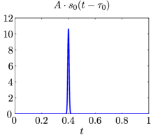
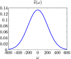
(a)	(b)

Figure 1: (a) The return signal for Gaussian pulse from (12) with $a=1/200$ and return parameters $A=1$ and $\tau_{0}=0.4$. (b) The Fourier transform $\widehat{s}(\omega)$ on $\Omega=[-600,600]$. Since $\widehat{s}$ is relatively diffuse over $\Omega$, both measures of frequency concentration are not too large: $\mu_{1}\leq 1.6,\leavevmode\nobreak\ \mu_{2}\leq 3.4$.

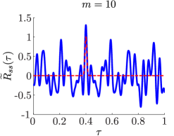
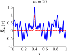
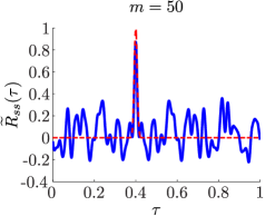
(a)	(b)	(c)

Figure 2: Estimated scaled, shifted autocorrelation function $\widetilde{R}_{ss}(\tau)$ (solid blue line) and true scaled, shifted autocorrelation function $A\cdot R_{ss}(\tau-\tau_{0})$ (dashed red line) for (a) $m=10$, (b) $m=20$, (c) and $m=50$ measurements. $\widetilde{R}_{ss}(\tau)$ is a random process whose mean is $A\cdot R_{ss}(\tau-\tau_{0})$; as the number of measurements increases, this process deviates less from its mean (see Theorems 1 and 2).

2.4 General Noiseless Performance Characterization

Our statements about about quantifying the number of samples needed to ensure a clear separation between the peak of $|\widetilde{R}_{ss}(\tau)|$ and the function away from the peak are easily generalized. The statements in this section can be interpreted as a condition on the number of samples needed to ensure the successful operation of the compressive matched filter. The result below is interesting when the underlying autocorrelation function $R_{ss}(\tau)$ has one main peak (a “main lobe”) centered at $\tau=0$, and is relatively small away from the origin. This situation is typical, but similar statements could be formulated depending on the assumptions one wishes to impose on $s(t)$ (and its autocorrelation function).

Corollary 3.

Suppose there exist constants $\alpha_{1}\in[0,1)$ and $\alpha_{2}>0$ such that $|R_{ss}(\tau)|\leq\alpha_{1}R_{ss}(0)$ for all $|\tau|>\alpha_{2}$, and choose $\epsilon\in[0,1-\alpha_{1}]$. Suppose also that $\left|\Omega\right|\left|T\right|\geq 3$ and that

$$m>C_{2}\cdot\max\left(\frac{\log(12|\Omega||T|/\delta)}{(1-\alpha_{1}-\epsilon)^{2}}\cdot\mu_{1}^{2},\;\frac{\sqrt{\log(4/\delta)\log(12|\Omega||T|/\delta)}}{1-\alpha_{1}-\epsilon}\cdot\mu_{2}\right),$$ (13)

where $C_{2}$ is a known universal constant. Then with probability at least $1-\delta$, $|\widetilde{R}_{ss}(\tau_{0})|>|\widetilde{R}_{ss}(\tau)|+\epsilon\eta$ for all $\tau$ such that $|\tau-\tau_{0}|>\alpha_{2}$.

Proof.

Supposing we have the concentration suggested by (11), we will have $|\widetilde{R}_{ss}(\tau_{0})|\geq|A|R_{ss}(0)-U$ and $|\widetilde{R}_{ss}(\tau)|\leq\alpha_{1}|A|R_{ss}(0)+U$ for all $\tau$ such that $|\tau-\tau_{0}|>\alpha_{2}$. If (13) is satisfied with $C_{2}=\max(4C_{1}^{2},2C_{1})$, then $U<\frac{1}{2}|A|R_{ss}(0)(1-\alpha_{1}-\epsilon)$ and it follows that $|A|R_{ss}(0)-U>\alpha_{1}|A|R_{ss}(0)+U+\epsilon|A|R_{ss}(0)$. A slightly stronger version of this corollary also holds if one omits $C_{2}$ and chooses constants of $4C_{1}^{2}$ and $2C_{1}$ for the first and second terms in (13), respectively. ∎

For the case of noiseless measurements, Corollary 3 ensures that no values of $\tau$ far from $\tau_{0}$ can give $|\widetilde{R}_{ss}(\tau)|$ close to $|\widetilde{R}_{ss}(\tau_{0})|$. This behavior will become particularly relevant in Section 2.5, where we introduce noise into the measurement process.

We can reveal some of the intuition behind the measurement bound (13) by considering three special cases for the signal $s$. First, consider $s(t)$ for which $|\widehat{s}(\omega)|$ is uniform over $\Omega$. In this case, we have $|\widehat{s}(\omega)|=|\Omega|^{-1/2}\|\widehat{s}\|_{2}$ for all $\omega\in\Omega$ and so $\mu_{1}=\mu_{2}=1$. This means that the requisite number of random measurements (13) for successful operation of the compressive matched filter scales as $m\sim\log(|\Omega||T|)$.

Alternatively, consider the case where $|\widehat{s}(\omega)|$ is not perfectly uniform over $\Omega$, but rather we assume that for some $\beta\geq 1$ it obeys $|\widehat{s}(\omega)|\leq\beta|\Omega|^{-1/2}\|\widehat{s}\|_{2}$ for all $\omega\in\Omega$, and so $\mu_{2}\leq\beta^{2}$. Using the fact that $\|\widehat{s}\|_{4}^{4}\leq\|\widehat{s}\|_{2}^{2}\|\widehat{s}\|_{\infty}^{2}$ gives us the estimate $\mu_{1}\leq\beta$. Therefore, (13) now demands that $m\sim\beta^{2}\log(|\Omega||T|)$ — the factor of $\beta^{2}$ is the price we pay for the non-uniformity of $\widehat{s}$.

As a final example, consider the special case where $s$ is bandlimited to some interval $\Omega_{B}\subseteq\Omega$ and $|\widehat{s}(\omega)|$ is uniform over $\Omega_{B}$, i.e.,

$$|\widehat{s}(\omega)|=\left\{\begin{array}[]{ll}\frac{\|\widehat{s}\|_{2}}{\sqrt{|\Omega_{B}|}},&\omega\in\Omega_{B}\\ 0,&\omega\in\Omega\backslash\Omega_{B},\end{array}\right.$$

One way we could interpret this situation is that we have chosen the sampling domain $\Omega$ to be too large. In this case, we have $\mu_{1}=\sqrt{|\Omega|/|\Omega_{B}|}$ and $\mu_{2}=|\Omega|/|\Omega_{B}|$, and so (13) now demands that $m\sim(|\Omega|/|\Omega_{B}|)\log(|\Omega||T|)$. The penalty $|\Omega|/|\Omega_{B}|$ is a natural oversampling factor since, on average, only $|\Omega_{B}|$ out of every $|\Omega|$ random Fourier samples will carry any information about the signal.

2.5 Robustness in the Presence of Measurement Noise

We now extend our analysis to account for additive complex-valued noise in our observations. For random frequencies $\{\omega_{k}\}$ taken uniformly from $\Omega$, we assume that the noisy measurement vector, $y_{n}$, is formed as

$$y_{n}[k]=Ae^{-\mathrm{i}\omega_{k}\tau_{0}}\widehat{s}_{0}(\omega_{k})+n_{k},\quad k=1,2,\ldots,m,$$

where the additive noise terms $\{n_{k}\}$ are independent zero-mean complex-valued Gaussian random variables with variance $\sigma_{n}^{2}$, and the noise vector is $n:=[n_{1},n_{2},...,n_{m}]^{T}$. Computing the inner product of $y_{n}$ with the test vector $\psi_{\tau}$ for all $\tau\in T$ leads us to the process

$$X_{n}(\tau):=\left\langle y_{n},\psi_{\tau}\right\rangle=X(\tau)+N(\tau),$$ (14)

where $X(\tau)$ is as defined in Section 2.2, and $N(\tau)$ is the noise process that quantifies the effect of additive noise in our analysis:

$$N(\tau):=\left\langle n,\psi_{\tau}\right\rangle=\sum_{k=1}^{m}n_{k}\widehat{s}_{0}^{*}(\omega_{k})e^{\mathrm{i}\omega_{k}\tau}=\sum_{k=1}^{m}n_{k}\widehat{s}^{*}(\omega_{k})e^{\mathrm{i}\omega_{k}\tau}.$$

The noise process is zero-mean, i.e., $\mathbb{E}N(\tau)=0$.

Thus, in the case of noisy observations, we can estimate the ideal autocorrelation function $R_{ss}(\cdot)$ (up to the unknown amplitude $A$ and translation $\tau_{0}$) simply by rescaling the noisy random process $X_{n}(\tau)$. Let us define

$$\widetilde{N}(\tau):=\left\{\begin{array}[]{ll}\frac{|\Omega|}{2\pi m}\cdot\mathrm{Re}(N(\tau)),&\mathrm{real\leavevmode\nobreak\ case},\\[2.84526pt] \frac{|\Omega|}{2\pi m}\cdot N(\tau),&\mathrm{complex\leavevmode\nobreak\ case},\end{array}\right.$$ (15)

and note that in either case, $\mathbb{E}[\widetilde{N}(\tau)]=0$. Then, if we set

$$\widetilde{R}_{ss,n}(\tau):=\left\{\begin{array}[]{ll}\frac{|\Omega|}{2\pi m}\cdot\mathrm{Re}(X_{n}(\tau)),&\mathrm{real\leavevmode\nobreak\ case},\\[2.84526pt] \frac{|\Omega|}{2\pi m}\cdot X_{n}(\tau),&\mathrm{complex\leavevmode\nobreak\ case},\end{array}\right.$$

it follows in either case that

$$\widetilde{R}_{ss,n}(\tau)=\widetilde{R}_{ss}(\tau)+\widetilde{N}(\tau),$$ (16)

where $\widetilde{R}_{ss}(\tau)$ is as defined in (7). This function provides an unbiased estimate of the shifted, scaled autocorrelation function of $s(t)$, since $\mathbb{E}[\widetilde{R}_{ss,n}(\tau)]=AR_{ss}(\tau-\tau_{0})$.

We can gain some intuition for how the noise is hindering the estimation process with a quick estimate on its expected size at a fixed point $\tau$. In both the real and complex cases, the variance of $\widetilde{N}(\tau)$ is bounded by

$$\operatorname{Var}\left[\widetilde{N}(\tau)\right] \leq\frac{|\Omega|^{2}}{4\pi^{2}m^{2}}\mathbb{E}\left|\sum_{k=1}^{m}n_{k}\widehat{s}^{*}(\omega_{k})e^{\mathrm{i}\omega_{k}\tau}\right|^{2}$$

$$=\frac{|\Omega|^{2}}{4\pi^{2}m^{2}}\sum_{k_{1}=1}^{m}\sum_{k_{2}=1}^{m}\mathbb{E}[n_{k_{1}}n_{k_{2}}^{*}]\mathbb{E}[\widehat{s}^{*}(\omega_{k_{1}})\widehat{s}(\omega_{k_{2}})e^{\mathrm{i}(\omega_{k_{1}}-\omega_{k_{2}})\tau}]$$

$$=\frac{|\Omega|^{2}}{4\pi^{2}m^{2}}\sum_{k=1}^{m}\mathbb{E}|n_{k}|^{2}\mathbb{E}|\widehat{s}(\omega_{k})|^{2}$$

$$=\frac{|\Omega|}{4\pi^{2}m}\sigma_{n}^{2}\|\widehat{s}\|_{2}^{2},$$

and so, using Jensen’s inequality, we obtain

$$\mathbb{E}|\widetilde{N}(\tau)|\leavevmode\nobreak\ \leq\leavevmode\nobreak\ \frac{1}{2\pi}\cdot\sigma_{n}\cdot\frac{\sqrt{|\Omega|}\|\widehat{s}\|_{2}}{\sqrt{m}}.$$ (17)

Recall that the peak of the noiseless estimate $|\widetilde{R}_{ss}(\tau)|$ is on the order of $\left|A\right|R_{ss}(0)=\left|A\right|(2\pi)^{-1}\|\widehat{s}\|_{2}^{2}$. Thus the noise process will overwhelm the peak of the noiseless estimate when

$$\sigma_{n}\leavevmode\nobreak\ \sim\leavevmode\nobreak\ \left|A\right|\|\widehat{s}\|_{2}\sqrt{\frac{m}{|\Omega|}}.$$ (18)

Theorems 4 and 5 below show that for $m$ large enough, we will have essentially the same bound as (17) hold uniformly over the entire search interval $T$. As a result, the amount of noise (size of $\sigma_{n}^{2}$) the compressive matched filter can withstand is essentially (to within constant and $\log$ factors) the same as in (18).

We start with a bound on the expected maximum of the noise process. The following result is proved in Section 4.2.

Theorem 4.

Suppose that $\left|\Omega\right|\left|T\right|\geq 3$. Then the noise process $\widetilde{N}(\tau)$, as defined in (15), obeys

$$\mathbb{E}\sup_{\tau\in T}\left|\widetilde{N}(\tau)\right| \leq\sigma_{n}\cdot\frac{\sqrt{|\Omega|}\|\widehat{s}\|_{2}}{\sqrt{m}}\cdot\left({0.199\sqrt{\log(|\Omega||T|)}}+0.166\right)$$

$$\leq 0.36\cdot\sigma_{n}\cdot\frac{\sqrt{|\Omega|}\|\widehat{s}\|_{2}}{\sqrt{m}}\cdot{\sqrt{\log(|\Omega||T|)}}.$$

The next theorem shows that, given $m$ large enough, the maximum of the noise process will not be too much larger than its mean with high probability. The following result is also proved in Section 4.2.

Theorem 5.

Fix $\delta>0$. Suppose that $\left|\Omega\right|\left|T\right|\geq 3$ and that

$$m\geq C_{3}\cdot\max\left(\mu_{1}^{2},\leavevmode\nobreak\ \mu_{2}\right)\cdot\log(1/\delta),$$ (19)

where $C_{3}$ is a known universal constant. Then the noise process $\widetilde{N}(\tau)$, as defined in (15), obeys

$$\operatorname{P}\left\{\sup_{\tau\in T}\left|\widetilde{N}\left(\tau\right)\right|\geq C_{4}\cdot\sigma_{n}\cdot\frac{\sqrt{|\Omega|}\|\widehat{s}\|_{2}}{\sqrt{m}}\cdot\max\left(\sqrt{\log(|\Omega||T|)},\sqrt{\log(2/\delta)}\right)\right\}\leavevmode\nobreak\ \leq\leavevmode\nobreak\ \delta,$$ (20)

where $C_{4}$ is a known universal constant.

These two theorems, taken in conjunction with Theorems 1 and 2, give us a bound on how far the estimate $\widetilde{R}_{ss,n}(\tau)$ created from noisy samples will vary from its mean. With high probability, we will have

$$\left|\widetilde{R}_{ss,n}(\tau)-AR_{ss}(\tau-\tau_{0})\right|\leavevmode\nobreak\ \lesssim\leavevmode\nobreak\ \max\left(\frac{\eta\mu_{1}}{\sqrt{m}},\leavevmode\nobreak\ \frac{\eta\mu_{2}}{m},\leavevmode\nobreak\ \frac{\sigma_{n}\sqrt{|\Omega|}\|\widehat{s}\|_{2}}{\sqrt{m}}\right)\cdot\sqrt{\log(|\Omega||T|)}.$$

Just as in the noiseless case, the bound on this deviation of our estimate of the autocorrelation function can be translated directly into a performance guarantee for the compressive matched filter. This is codified in the following corollary.

Corollary 6.

Suppose there exist constants $\alpha_{1}\in[0,1)$ and $\alpha_{2}>0$ such that $|R_{ss}(\tau)|\leq\alpha_{1}R_{ss}(0)$ for all $|\tau|>\alpha_{2}$. Suppose also that $\left|\Omega\right|\left|T\right|\geq 3$, that (19) is satisfied, and that

$$m> \;C_{5}\cdot\max\left(\frac{\log(12|\Omega||T|/\delta)}{(1-\alpha_{1})^{2}}\cdot\mu_{1}^{2},\;\frac{\sqrt{\log(4/\delta)\log(12|\Omega||T|/\delta)}}{1-\alpha_{1}}\cdot\mu_{2},\right.$$

$$\leavevmode\nobreak\ \leavevmode\nobreak\ \leavevmode\nobreak\ \leavevmode\nobreak\ \leavevmode\nobreak\ \leavevmode\nobreak\ \leavevmode\nobreak\ \leavevmode\nobreak\ \leavevmode\nobreak\ \leavevmode\nobreak\ \leavevmode\nobreak\ \leavevmode\nobreak\ \leavevmode\nobreak\ \left.\frac{\max\left(\log(|\Omega||T|),\log(2/\delta)\right)}{(1-\alpha_{1})^{2}}\cdot\frac{\sigma_{n}^{2}|\Omega|}{|A|^{2}\|\widehat{s}\|_{2}^{2}}\right),$$ (21)

where $C_{5}$ is a known universal constant. Then with probability at least $1-2\delta$, the maximum value of $|\widetilde{R}_{ss,n}(\tau)|$ must be attained for some $\widehat{\tau}_{0}$ within the interval $[\tau_{0}-\alpha_{2},\tau_{0}+\alpha_{2}]$.

Proof.

Using (16), we have that

$$\sup_{\tau}|\widetilde{R}_{ss,n}(\tau)-AR_{ss}(\tau-\tau_{0})|\leq\sup_{\tau}|\widetilde{R}_{ss}(\tau)-AR_{ss}(\tau-\tau_{0})|+\sup_{\tau}|\widetilde{N}(\tau)|,$$

where $\widetilde{R}_{ss}(\tau)$ is defined in (7). With probability at least $1-2\delta$, both (11) and (20) will be satisfied, and so we will have

$$|\widetilde{R}_{ss,n}(\tau_{0})|\geq\left|A\right|\frac{\|\widehat{s}\|_{2}^{2}}{2\pi}-U-\frac{C_{4}\sigma_{n}\sqrt{|\Omega|}\|\widehat{s}\|_{2}\max\left(\sqrt{\log(|\Omega||T|)},\sqrt{\log(2/\delta)}\right)}{\sqrt{m}}$$ (22)

and

$$|\widetilde{R}_{ss,n}(\tau)|\leq\alpha_{1}\left|A\right|\frac{\|\widehat{s}\|_{2}^{2}}{2\pi}+U+\frac{C_{4}\sigma_{n}\sqrt{|\Omega|}\|\widehat{s}\|_{2}\max\left(\sqrt{\log(|\Omega||T|)},\sqrt{\log(2/\delta)}\right)}{\sqrt{m}}$$ (23)

for all $\tau$ such that $|\tau-\tau_{0}|>\alpha_{2}$. If (21) is satisfied with $C_{5}=\max(16C_{1}^{2},4C_{1},64\pi^{2}C_{4}^{2})$, then it follows that the right hand side of (22) must exceed the right hand side of (23). As with Corollary 3, one can slightly strengthen this result by choosing differing constants for the three terms appearing in (21). ∎

To within a constant factor, the first two terms in (21) are the same as in Corollary 3; we might think of these terms as “activation” conditions for when the compressive matched filter will be well-behaved in the absence of noise. After these conditions are met, it can withstand noise levels up to a size

$$\sigma_{n}\leavevmode\nobreak\ \sim\leavevmode\nobreak\ \left|A\right|\|\widehat{s}\|_{2}\sqrt{\frac{m}{|\Omega|\log(|\Omega||T|)}}.$$ (24)

We can interpret (18) as the noise level at which the operation of the compressive matched filter will fall apart completely, and (24) (which is only a log factor smaller) as the noise level at which we have guaranteed accuracy.

Three examples of the estimated autocorrelation function $\widetilde{R}_{ss,n}(\tau)$ are shown in Figure 3 for the Gaussian pulse example from Section 2.3 with a fixed number $m=50$ of samples and various values of $\sigma_{n}^{2}$ (the noiseless estimates $\widetilde{R}_{ss}(\tau)$ are overlaid). For the same number of measurements, Figure 4 shows the average performance of the compressive matched filter versus the noise level. For various noise levels $\sigma_{n}$ between $0$ and $|A|\|\widehat{s}\|_{2}\sqrt{m/|\Omega|}$, we run 1000 experiments generating random sample frequencies and random noise, and estimate $\tau_{0}$ by identifying the peak of $|\widetilde{R}_{ss,n}(\tau)|$. The figure indicates the percentage of trials in which the delay was estimated to within a distance $2a$ of the correct value $\tau_{0}$. We see in these experiments that the estimator begins to lose effectiveness roughly when $\sigma_{n}\sim 0.25\cdot|A|\|\widehat{s}\|_{2}\sqrt{m/|\Omega|}$.

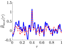
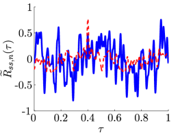
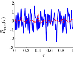
(a)	(b)	(c)

Figure 3: Estimated scaled, shifted autocorrelation function $\widetilde{R}_{ss,n}(\tau)$ (solid blue line) obtained from noisy samples, and for the sake of comparison, the estimate $\widetilde{R}_{ss}(\tau)$ (dashed red line) that would have been obtained without noise. For all experiments, the number of samples $m=50$, and the noise level (a) $\sigma_{n}=0.2\cdot|A|\|\widehat{s}\|_{2}\sqrt{m/|\Omega|}$, (b) $\sigma_{n}=0.5\cdot|A|\|\widehat{s}\|_{2}\sqrt{m/|\Omega|}$, and (c) $\sigma_{n}=|A|\|\widehat{s}\|_{2}\sqrt{m/|\Omega|}$. Overall, the time-of-arrival estimation is reliable in the first case, tenuous in the second case, and completely unreliable in the third case.

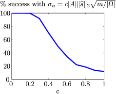
Figure 4: Percentage of correct time-of-arrival estimation ($|\widehat{\tau}_{0}-\tau_{0}|\leq 2a$) over 1000 trials, as a function of the noise level $\sigma_{n}=c\cdot|A|\|\widehat{s}\|_{2}\sqrt{m/|\Omega|}$, $0\leq c\leq 1$.

It is worth recalling that a user may have some control over selecting the observation interval $\Omega$. In most cases it would be natural to choose $\Omega$ roughly equal to the essential bandwidth of $s_{0}$. Taking $\Omega$ larger than this will increase $\mu_{1}$, $\mu_{2}$, and the sensitivity to noise; taking $\Omega$ smaller than this will generally increase the width of the main lobe of the autocorrelation function $R_{ss}(\tau)$ and thus limit the resolution to which $\tau_{0}$ can be estimated.

Finally, we can compare the noise levels in (18) and (24) to the noise levels at which a digital matched filter working from a set of samples taken in the time domain at the Nyquist rate $|\Omega|/2\pi$ will stop being effective. Suppose we sample the (bandlimited) return signal $As(t-\tau_{0})$ at the Nyquist rate, and noise is added to these samples. We observe

$$y_{d}[\ell]=As_{d,\tau_{0}}[\ell]+n_{d}[\ell],\quad\text{where}\quad s_{d,\tau_{0}}[\ell]=\left.s(t-\tau_{0})\right|_{t=\ell 2\pi/|\Omega|},$$

and $n_{d}[\ell]$ is sequence of independent zero-mean Gaussian random variables with variances $\sigma_{n}^{2}|\Omega|/2\pi$. This variance is chosen to make the noise process similar to that analyzed in the compressive case; it corresponds to samples of a continuous-time process that has a power spectral density equal to $\sigma_{n}^{2}$ on $\Omega$ and zero elsewhere.

Focusing just on the complex case for the sake of brevity, once we have collected $y_{d}$, we can estimate the scaled, shifted autocorrelation function using

$$\widetilde{R}_{d}(\tau)=\langle y_{d},s_{d,\tau}\rangle=A\langle s_{d,\tau_{0}},s_{d,\tau}\rangle+\langle n_{d},s_{d,\tau}\rangle$$ (25)

and choose as our estimate of $\tau_{0}$ the maximizer of $|\widetilde{R}_{d}(\tau)|$ over all $\tau$. At the correct shift $\tau_{0}$, the first inner product in (25) is given by

$$\langle s_{d,\tau_{0}},s_{d,\tau_{0}}\rangle=\sum_{\ell}|s_{d,\tau_{0}}[\ell]|^{2}=\frac{|\Omega|}{2\pi}\|s(t-\tau_{0})\|_{2}^{2}=\frac{|\Omega|}{4\pi^{2}}\|\widehat{s}\|_{2}^{2},$$

where the second equality comes from the fact that $s(\cdot)$ is bandlimited and we are sampling at the Nyquist rate. The second inner product is a Gaussian random variable with

$$\operatorname{Var}\left[\langle n_{d},s_{d,\tau}\rangle\right]\leavevmode\nobreak\ =\leavevmode\nobreak\ \frac{\sigma_{n}^{2}|\Omega|}{2\pi}\sum_{\ell}|s_{d,\tau}[\ell]|^{2}\leavevmode\nobreak\ =\leavevmode\nobreak\ \frac{\sigma_{n}^{2}|\Omega|^{2}}{8\pi^{3}}\|\widehat{s}\|_{2}^{2},$$

and so

$$\mathbb{E}|\langle n_{d},s_{d,\tau}\rangle|\leavevmode\nobreak\ \leq\leavevmode\nobreak\ \frac{\sigma_{n}|\Omega|}{2\pi\sqrt{2\pi}}\cdot\|\widehat{s}\|_{2}.$$

Roughly speaking, then, the Nyquist sampled matched filter will be overwhelmed by the noise when

$$\sigma_{n}\leavevmode\nobreak\ \sim\leavevmode\nobreak\ \left|A\right|\|\widehat{s}\|_{2}.$$ (26)

Comparing (26) to the compressive matched filter results (18) and (24), we can interpret the factor of $\sqrt{m/|\Omega|}$ as a sort of undersampling penalty; as the number of samples gets smaller, the noise tolerance gets worse. When $m\gtrsim|\Omega|$, the performance of the two schemes will be similar. (A similar undersampling penalty arises in standard CS [8], where the noise variance that can be tolerated for a given recovery error decreases as the number of measurements gets smaller.)

3 Pure Tone Estimation

As discussed in Section 1.2.3, the roles of time and frequency are completely interchangeable in our settings. This allows us to apply the compressive matched filter to the problem of finding the carrier frequency of a modulated signal from time-domain samples with minimal effort. One particular such application is studied here: estimating the frequency of a pure tone from random samples in time.

Formally the problem under study is described as follows. A pure exponential $Ae^{\mathrm{i}\omega_{0}t}$ with fixed—but unknown—frequency $\omega_{0}\in\Omega$, amplitude $|A|$, and phase $\measuredangle A$ is observed on $T=[-t_{\mathrm{max}},t_{\mathrm{max}}]$. Let $y$ be the vector of observations at sampling times $t_{1},t_{2},...,t_{m}\in T$, which are randomly chosen from a uniform distribution on $T$, i.e.,

$$y=A\left[\begin{array}[]{c}e^{\mathrm{i}\omega_{0}t_{1}}\\ e^{\mathrm{i}\omega_{0}t_{2}}\\ \vdots\\ e^{\mathrm{i}\omega_{0}t_{m}}\end{array}\right].$$

Given $y\in\mathbb{C}^{m}$, we are interested in estimating $\omega_{0}\in\Omega$ and $A\in\mathbb{C}$. A natural approach to solving this problem is to find the find $\omega_{0}$ and $A$ which best explain the measurements in a least-squares sense. More formally, we define

$$(\widehat{\omega}_{0},\widehat{A}):=\arg\min_{\omega,A}\sum_{k=1}^{m}\left|y[k]-A\cdot e^{\mathrm{i}\omega t_{k}}\right|^{2}=\arg\min_{\omega,A}\|y-A\psi_{\omega}\|_{2}^{2},$$ (27)

where for any $\omega\in\Omega$, the test vector $\psi_{\omega}\in\mathbb{C}^{m}$ is given by:

$$\psi_{\omega}[k]=e^{\mathrm{i}\omega t_{k}},\quad k=1,2,\ldots,m.$$

The least-squares solution for $\omega_{0}$ is given by

$$\widehat{\omega}_{0}=\arg\max_{\omega\in\Omega}\left|\langle y,\psi_{\omega}\rangle\right|,$$ (28)

and subsequent to estimating $\omega_{0}$, the least-squares estimate for $A$ can be computed as $\widehat{A}=\langle y,\psi_{\widehat{\omega}_{0}}\rangle\|\psi_{\widehat{\omega}_{0}}\|_{2}^{-2}$.

3.1 Analytical Framework

Equation (28) suggests a correlation-based strategy for estimating the unknown frequency $\omega_{0}$. In order to study the performance of such an estimator, let us define the random process $X(\omega):=\left\langle y,\psi_{\omega}\right\rangle$ on $\Omega$, which has the mean function

$$\mathbb{E}X(\omega) =A\mathbb{E}\sum_{k=1}^{m}e^{\mathrm{i}(\omega_{0}-\omega)t_{m}}$$

$$=A\sum_{k=1}^{m}\mathbb{E}e^{\mathrm{i}(\omega_{0}-\omega)t_{m}}$$

$$=mA\left|T\right|^{-1}\int_{T}e^{\mathrm{i}(\omega_{0}-\omega)t}\leavevmode\nobreak\ dt$$

$$=mA|T|^{-1}\cdot|T|\mbox{sinc}\left(\frac{1}{2}\left|T\right|(\omega_{0}-\omega)\right),$$

where $\mbox{sinc}\left(\alpha\right):=\sin\left(\alpha\right)/\alpha$. One way to interpret $X(\omega)$ is that we have approximated the continuous-time inner product between two time-limited complex sinusoids as a discrete sum with samples taken at random locations; the above tells us that this estimate is unbiased.

Further attention reveals that we are facing the same problem as in the complex case of Section 2, where the roles of time and frequency have been interchanged: the frequency domain becomes the “shift domain,” while the time domain becomes the “observation domain.” More precisely, we may define $\widehat{s}_{0}(\omega)=2\pi\delta(\omega)$ which has the inverse Fourier transform $s_{0}(t)=1$. Our received signal can be expressed in the frequency domain as $A\cdot\widehat{s}_{0}(\omega-\omega_{0})$ for some $\omega_{0}\in\Omega$. However, we will observe $m$ samples of this signal in the time domain, acquiring values of $Ae^{\mathrm{i}\omega_{0}t}s_{0}(t)=Ae^{\mathrm{i}\omega_{0}t}$ at times $t_{1},t_{2},\dots,t_{m}\in T$.

Now, in the observation (time) domain, we define $s(t)$ to be the time-limited version of $s_{0}(t)$, i.e., $s(t):=\mathbb{I}_{t\in T}$ where $\mathbb{I}$ denotes the indicator function. Returning to the shift (frequency) domain, we have $\widehat{s}(\omega)=|T|\mbox{sinc}\left(\frac{1}{2}\left|T\right|\omega\right)$. Up to a constant factor, this expression equals its own autocorrelation function, i.e., $R_{\widehat{s}\widehat{s}}(\omega)=2\pi\widehat{s}(\omega)$.

Therefore, we can estimate the ideal autocorrelation function $R_{\widehat{s}\widehat{s}}(\cdot)$ (up to the unknown complex amplitude $A$ and translation $\omega_{0}$) by rescaling the random process $X(\omega)$:

$$\widetilde{R}_{\widehat{s}\widehat{s}}(\omega):=\frac{2\pi|T|}{m}X(\omega).$$ (29)

This estimate is unbiased since $\mathbb{E}[\widetilde{R}_{\widehat{s}\widehat{s}}(\omega)]=A\cdot R_{\widehat{s}\widehat{s}}(\omega-\omega_{0})$. It is clear that solving the least-squares problem (28) is equivalent to searching for the maximizer of $|\widetilde{R}_{\widehat{s}\widehat{s}}(\omega)|$. Since the the main lobe of $R_{\widehat{s}\widehat{s}}(\omega)=2\pi|T|\mbox{sinc}\left(\frac{1}{2}\left|T\right|\omega\right)$ is centered at the origin (with $R_{\widehat{s}\widehat{s}}(0)=2\pi|T|$), we informally expect that, on average, finding the maximum of $|\widetilde{R}_{\widehat{s}\widehat{s}}(\omega)|$ correctly estimates $\omega_{0}$.

3.2 Noiseless Analysis

To study the concentration of $\widetilde{R}_{\widehat{s}\widehat{s}}(\omega)$ about its mean, we may follow the same arguments as in Sections 2.2 and 2.4 while simply exchanging the roles of time and frequency. In particular, we note that the problem of pure tone estimation corresponds to the first “special case” studied in Section 2.4, because the windowed signal template has uniform magnitude in the observation domain. Thus, we have $\mu_{1}=\mu_{2}=1$. This leads us to the following result for the case of noiseless observations.

Corollary 7.

Fix $\delta>0$ and let

$$U=2\pi C_{1}|A||T|\cdot\max\left(\frac{1}{\sqrt{m}},\leavevmode\nobreak\ \frac{\sqrt{\log(4/\delta)}}{m}\right)\cdot\sqrt{\log(12|\Omega||T|/\delta)}.$$

If $\left|\Omega\right|\left|T\right|\geq 3$, then the estimate of the autocorrelation function in (29) obeys

$$\Pr\left\{\sup_{\omega\in\Omega}\left|\widetilde{R}_{\widehat{s}\widehat{s}}(\omega)-AR_{\widehat{s}\widehat{s}}(\omega-\omega_{0})\right|>U\right\}\leq\delta.$$

This corollary follows immediately from Theorem 2.

A close inspection of the definition of $\widetilde{R}_{\widehat{s}\widehat{s}}(\omega)$ reveals that $\omega_{0}$ is guaranteed to be a maximizer of $|\widetilde{R}_{\widehat{s}\widehat{s}}(\omega)|$, with $|\widetilde{R}_{\widehat{s}\widehat{s}}(\omega_{0})|=2\pi|A||T|$. What Corollary 7 ensures is that even for small values of $m$, no other values of $\omega$ far from $\omega_{0}$ can give $|\widetilde{R}_{\widehat{s}\widehat{s}}(\omega)|$ equal (or even close to) $|\widetilde{R}_{\widehat{s}\widehat{s}}(\omega_{0})|$. This fact is not only useful when we introduce nonidealities into the observation process (see Section 3.4) but also in guiding a computational method to search for the peak of $|\widetilde{R}_{\widehat{s}\widehat{s}}(\omega)|$. We investigate this issue in Section 3.3 below.

3.3 A Grid Search Approach

In practice, in order to find the peak of $|\widetilde{R}_{\widehat{s}\widehat{s}}(\omega)|$, one might hope to simply sample this function over a uniformly spaced grid of frequencies drawn from $\Omega$. Because $\widetilde{R}_{\widehat{s}\widehat{s}}(\omega)$ is guaranteed to remain close to $AR_{\widehat{s}\widehat{s}}(\omega-\omega_{0})$, which decays sharply away from $\omega_{0}$, it is possible to guarantee that as long as the grid is chosen sufficiently fine, then the empirical maximum over the grid points will occur very close to the true peak.

To illustrate this fact with some specific but arbitrary values, let us note that for $|\omega|\leq\pi|T|^{-1}$, $|R_{\widehat{s}\widehat{s}}(\omega)|\geq 0.636\cdot 2\pi|T|$. Moreover, for $|\omega|\geq 2\pi|T|^{-1}$, $|R_{\widehat{s}\widehat{s}}(\omega)|\leq 0.218\cdot 2\pi|T|$. Following the techniques used to prove Corollary 3, we can ensure that $0.636\cdot 2\pi\left|A\right||T|-U>0.218\cdot 2\pi\left|A\right||T|+U$ with probability at least $1-\delta$ by taking

$$m\geq C_{2}\cdot\max\left(\frac{\log(12|\Omega||T|/\delta)}{(0.636-0.218)^{2}},\;\frac{\sqrt{\log(4/\delta)\log(12|\Omega||T|/\delta)}}{(0.636-0.218)}\right).$$

It follows that, if we initially search for the maximum of $|R_{\widehat{s}\widehat{s}}(\omega)|$ on a grid with resolution $2\pi|T|^{-1}$ (note that this is the so-called grid of Nyquist frequencies, given $T$), we are guaranteed that the empirical maximum will occur at a grid point $\widehat{\omega}_{0}$ such that $|\widehat{\omega}_{0}-\omega_{0}|<2\pi|T|^{-1}$.

After this initial grid search, it is actually straightforward to refine the accuracy of the estimate $\widehat{\omega}_{0}$ using a local concave ascent. Note that

$$\left|\widetilde{R}_{\widehat{s}\widehat{s}}(\omega)\right|^{2} =\left(\frac{2\pi|T|}{m}\right)^{2}\left|\left\langle y,\psi_{\omega}\right\rangle\right|^{2}$$

$$=\left(\frac{2\pi|T||A|}{m}\right)^{2}\sum_{i,j}e^{\mathrm{i}\left(\omega_{0}-\omega\right)\left(t_{i}-t_{j}\right)}$$

$$=\frac{\left(2\pi|T||A|\right)^{2}}{m}+\left(\frac{2\pi|T||A|}{m}\right)^{2}\sum_{i\neq j}\cos\left(\left(\omega_{0}-\omega\right)\left(t_{i}-t_{j}\right)\right).$$

Since $|t_{i}-t_{j}|\leq|T|$, $|\widetilde{R}_{\widehat{s}\widehat{s}}(\omega)|^{2}$ is guaranteed to be a concave function of $\omega$ when $|\omega-\omega_{0}|\leq\frac{\pi}{2}\cdot|T|^{-1}$. Therefore, if we have an estimate $\widehat{\omega}_{0}$ sufficiently close to the true $\omega_{0}$ (i.e., $|\widehat{\omega}_{0}-\omega_{0}|\leq\frac{\pi}{2}\cdot|T|^{-1}$), a standard concave maximization (akin to convex minimization) procedure beginning at $|\widetilde{R}_{\widehat{s}\widehat{s}}(\widehat{\omega}_{0})|$ will give us the exact value for $\omega_{0}$. Since the grid search above guarantees that $|\widehat{\omega}_{0}-\omega_{0}|<2\pi|T|^{-1}$, one could ensure success by running four concave maximizations starting from the points $\widehat{\omega}_{0}\pm\frac{\pi}{2}\cdot|T|^{-1}$ and $\widehat{\omega}_{0}\pm\frac{3\pi}{2}\cdot|T|^{-1}$.

3.4 Robustness

It is also possible to consider nonidealities in the observation process. Following the same set of arguments as in Section 2.5 (but exchanging the roles of time and frequency), we arrive at the following result.

Corollary 8.

Let $N(\omega)$ denote the random process induced by additive complex-valued Gaussian measurement noise having variance $\sigma_{n}^{2}$, and define

$$\widetilde{R}_{\widehat{s}\widehat{s},n}(\omega):=\frac{2\pi|T|}{m}(X(\omega)+N(\omega))$$

to be the estimate of the autocorrelation function formed using the noisy samples. Let $\delta>0$. Suppose that $\left|\Omega\right|\left|T\right|\geq 3$, that $m\geq C_{3}\log(1/\delta)$, and that

$$m\geq C_{5}\cdot\max\left(\frac{\log(12|\Omega||T|/\delta)}{(1-0.218)^{2}},\;\frac{\sqrt{\log(4/\delta)\log(12|\Omega||T|/\delta)}}{1-0.218},\;\frac{\max\left(\log(|\Omega||T|),\log(2/\delta)\right)}{(1-0.218)^{2}}\cdot\frac{\sigma_{n}^{2}}{|A|^{2}}\right).$$

Then with probability at least $1-2\delta$, the maximum value of $|\widetilde{R}_{\widehat{s}\widehat{s},n}(\omega)|$ must be attained for some $\widehat{\omega}_{0}$ within the interval $[\omega_{0}-2\pi|T|^{-1},\omega_{0}+2\pi|T|^{-1}]$.

Finally, let us note that with some additional work, we believe it would be possible to extend our analysis to account for multiple tones (or multiple translated pulses in the context of Section 2). The problem becomes that of detecting the true peaks in a noisy sum of $\mathrm{sinc}$ functions. For tones that are well-separated, one could argue that the interference in the random process is minimal and that any prominent peak in $|\widetilde{R}_{\widehat{s}\widehat{s},n}(\omega)|$ indicates the presence of a tone. Tones that are very close may be impossible to discriminate (this is true even with Nyquist-rate samples), while tones that are moderately separated may be possible to discriminate by employing a greedy, iterative estimation procedure.

3.5 Stylized Application: Chirp Time-of-Arrival Estimation

We close by noting that the ability to estimate a pure tone’s frequency from random time samples can also be parlayed into a technique for estimating a chirp signal’s time-of-arrival from random time samples. For this discussion, suppose we receive a chirp signal

$$x(t)=A\exp\left(j\left(\omega_{c}(t-t_{0})+\frac{\alpha}{2}(t-t_{0})^{2}\right)\right)$$

over some time interval, where $\omega_{c}$ denotes the known starting frequency, $\alpha$ denotes the known chirp rate, $A$ denotes the complex amplitude, and $t_{0}$ denotes the unknown time-of-arrival. We can “de-chirp” this signal over this interval, computing

$$\widetilde{x}(t)=x(t)\exp\left(-j\left(\omega_{c}t+\frac{\alpha}{2}t^{2}\right)\right)=\tilde{A}e^{-j\alpha t_{0}t},$$

where $\tilde{A}$ is a complex amplitude. The signal $\widetilde{x}(t)$ is merely a complex sinusoid (in this case, with frequency $\alpha t_{0}$). We have argued in this section that it is possible to estimate a pure tone’s frequency from random samples in time, and in this case that means that it is possible to estimate the time-of-arrival parameter $t_{0}$ from random samples of $\widetilde{x}(t)$ in time. It is important to note that time samples of $\widetilde{x}(t)$ can be computed easily from time samples of $x(t)$ itself, since the two signals are related via point-wise multiplication.

4 Theory

4.1 Proofs of Theorems 1 and 2 (Noiseless Analysis)

Let us begin by noting that, in the real case, both Theorems 1 and 2 are concerned with bounding

$$\left|\widetilde{R}_{ss}(\tau)-AR_{ss}(\tau-\tau_{0})\right| = \left|\widetilde{R}_{ss}(\tau)-A\cdot\mathrm{Re}(R_{ss}(\tau-\tau_{0}))\right|$$ (30a)

$$= \left|\frac{|\Omega|}{2\pi m}\cdot\mathrm{Re}(X(\tau))-\frac{|\Omega|}{2\pi m}\cdot\mathrm{Re}(\mathbb{E}X(\tau))\right|$$

$$= \frac{|\Omega|}{2\pi m}\left|\mathrm{Re}\left(X(\tau)-\mathbb{E}X(\tau)\right)\right|$$

$$\leq \frac{|\Omega|}{2\pi m}\left|X(\tau)-\mathbb{E}X(\tau)\right|.$$

In the complex case, both theorems are concerned with bounding

$$\left|\widetilde{R}_{ss}(\tau)-AR_{ss}(\tau-\tau_{0})\right| = \frac{|\Omega|}{2\pi m}\left|X(\tau)-\mathbb{E}X(\tau)\right|.$$ (30b)

Thus, to cover both cases, it suffices to focus on bounding $\left|X(\tau)-\mathbb{E}X(\tau)\right|$.

4.1.1 Setup

The first step in our approach to bounding $\left|X(\tau)-\mathbb{E}X(\tau)\right|$ is to define the centered process

$$Y(\tau):=X(\tau)-\mathbb{E}X(\tau)=A\sum_{k=1}^{m}\left|\widehat{s}\left(\omega_{k}\right)\right|^{2}e^{\mathrm{i}\omega_{k}\left(\tau-\tau_{0}\right)}-2\pi Am|\Omega|^{-1}R_{ss}(\tau-\tau_{0}).$$

Our goal is to bound $\sup_{\tau}|Y(\tau)|$, but to do this, we relate the random process to one that is more easily bounded. First, we symmetrize $Y(\tau)$ in the standard way. Create an independent copy $Y^{\prime}(\tau)$ (generated from an independent set of samples $\omega_{1}^{\prime},\omega_{2}^{\prime}\ldots,\omega_{m}^{\prime}$), and define

$$Z(\tau) :=Y(\tau)-Y^{\prime}(\tau)$$

$$=A\sum_{k=1}^{m}|\widehat{s}(\omega_{k})|^{2}e^{\mathrm{i}\omega_{k}(\tau-\tau_{0})}-|\widehat{s}(\omega_{k}^{\prime})|^{2}e^{\mathrm{i}\omega_{k}^{\prime}(\tau-\tau_{0})}.$$ (31)

Each term in (31) is a symmetric random variable, and so $Z(\tau)$ has the same distribution as

$$Z^{\prime}(\tau):=A\sum_{k=1}^{m}\epsilon_{k}\left(\left|\widehat{s}(\omega_{k})\right|^{2}e^{\mathrm{i}\omega_{k}(\tau-\tau_{0})}-\left|\widehat{s}(\omega_{k}^{\prime})\right|^{2}e^{\mathrm{i}\omega_{k}^{\prime}(\tau-\tau_{0})}\right),$$

where $\epsilon_{1},\epsilon_{2},...,\epsilon_{m}$ is a Rademacher sequence independent of everything.

We can control $\mathbb{E}\sup_{\tau}|Y(\tau)|$ through $\mathbb{E}\sup_{\tau}|Z^{\prime}(\tau)|$ using the following simple result, which is proved in Appendix A.

Lemma 9.

$\mathbb{E}\sup_{\tau}|Y(\tau)|\leq\mathbb{E}\sup_{\tau}|Z^{\prime}(\tau)|$.

Furthermore, the deviation of $\sup_{\tau}|Y(\tau)|$ from its average can be controlled through the corresponding deviation of $\sup_{\tau}|Z^{\prime}(\tau)|$. The following is proved in Appendix B.

Lemma 10.

For any $\lambda\geq 0$,

$$\operatorname{P}\left\{\sup_{\tau}|Y(\tau)|>2\mathbb{E}\sup_{\tau}|Y(\tau)|+\lambda\right\}\leavevmode\nobreak\ \leq\leavevmode\nobreak\ 2\operatorname{P}\left\{\sup_{\tau}|Z^{\prime}(\tau)|>\lambda\right\}.$$

The above results allow us to focus on developing expectation and tail bounds for $\sup_{\tau}|Z^{\prime}(\tau)|$. We establish such bounds in the following subsections.

To ease the notation below, we make the following definitions for quantities that will appear often:

$$M=M(s):=\sup_{\omega\in\Omega}|\widehat{s}(\omega)|^{2}=\|\widehat{s}\|_{\infty}^{2},$$

$$M_{1}=M_{1}(s,m,\Omega):=\sqrt{\frac{m}{|\Omega|}}\|\widehat{s}\|_{4}^{2},$$

$$M_{2}=M_{2}(s,m,\Omega):=\sqrt{\frac{m}{|\Omega|}}\|\widehat{s}\|_{2},$$

$$M_{3}=M_{3}(s,\omega_{1},\omega_{2},\dots,\omega_{m},\omega_{1}^{\prime},\omega_{2}^{\prime},\dots,\omega_{m}^{\prime}):=\sqrt{\sum_{k=1}^{m}|\widehat{s}(\omega_{k})|^{4}+|\widehat{s}(\omega_{k}^{\prime})|^{4}},$$

and

$$M_{4}=M_{4}(s,\omega_{1},\omega_{2},\dots,\omega_{m}):=\sqrt{\sum_{k=1}^{m}|\widehat{s}(\omega_{k})|^{2}}.$$

We will also frequently use the following convenient facts. For any $a$ and $b$, we have

$$e^{\mathrm{i}a}-e^{\mathrm{i}b}=2\mathrm{i}\sin\left(\frac{a-b}{2}\right)e^{\mathrm{i}(a+b)/2},$$ (32)

and

$$\left|a+b\right|^{2}\leq 2\left|a\right|^{2}+2\left|b\right|^{2}.$$ (33)

Also, for any $c,u>0$, the following inequality follows from a standard Gaussian tail bound [19]:

$$\int_{x\geq u}e^{-\frac{x^{2}}{c^{2}}}dx\leq\frac{c^{2}}{2u}e^{-\frac{u^{2}}{c^{2}}}.$$ (34)

4.1.2 Chaining

We start by bounding $\sup_{\tau}\left|Z^{\prime}(\tau)\right|$ conditioned on the choice of $\{\omega_{k}\}$ and $\{\omega^{\prime}_{k}\}$. To this end, we will use a chaining argument similar to what is used to prove the general Dudley inequality [12], but optimized for our particular process (this will allow us to tightly control the constants).

The following tail bounds for $Z^{\prime}(\tau)$ and its increments are proved in Appendix C.

Lemma 11.

For a fixed $\tau\in\mathbb{R}$ and any $\lambda\geq 0$, $Z^{\prime}(\tau)$ obeys

$$\operatorname{P}_{\epsilon_{k}}\left\{|Z^{\prime}(\tau)|>\lambda\right\}\leavevmode\nobreak\ \leq\leavevmode\nobreak\ 2\exp\left(-\frac{\lambda^{2}}{4|A|^{2}M_{3}^{2}}\right),$$ (35)

where $\operatorname{P}_{\epsilon_{k}}$ denotes probability with respect to $\{\epsilon_{k}\}$ conditioned on fixed $\{\omega_{k}\}$ and $\{\omega^{\prime}_{k}\}$. Also, for fixed $\tau_{1},\tau_{2}\in\mathbb{R}$,

$$\operatorname{P}_{\epsilon_{k}}\left\{|Z^{\prime}(\tau_{1})-Z^{\prime}(\tau_{2})|>\lambda\right\}\leavevmode\nobreak\ \leq\leavevmode\nobreak\ 2\exp\left(-\frac{\lambda^{2}}{|A|^{2}M_{3}^{2}|\Omega|^{2}|\tau_{1}-\tau_{2}|^{2}}\right).$$ (36)

We will consider the values of $Z^{\prime}(\tau)$ on a series of discrete grids of points that are essentially localized on the interval $T=[\tau_{\mathrm{min}},\tau_{\mathrm{max}}]$. For each integer $j\geq 0$, let $T_{j}$ be a grid of points spaced $2^{-j}|\Omega|^{-1}$ apart:

$$T_{j}=\{\tau_{\mathrm{min}}+2^{-j-1}|\Omega|^{-1}+k2^{-j}|\Omega|^{-1},\leavevmode\nobreak\ k=0,1,\ldots,\lfloor 2^{j}|\Omega||T|\rfloor\}.$$ (37)

All points in $T_{j}$ belong to $T$, except possibly the final point in $T_{j}$, which may exceed $\tau_{\mathrm{max}}$ by no more than $2^{-j-1}|\Omega|^{-1}$. Moreover, if we denote by $\pi_{j}(\tau)$ the closest point in $T_{j}$ to a given point $\tau$, then $|\tau-\pi_{j}(\tau)|\leq 2^{-j-1}|\Omega|^{-1}$ for all $\tau\in T$. The points in the $T_{j}$ are arranged like nodes in a dyadic tree, with each “parent” in $T_{j}$ having two “children” in $T_{j+1}$ (the two points that are closer to the parent than to any other point in $T_{j}$); the only exception to this rule occurs if $|T_{j+1}|$ is odd, in which case the final point in $T_{j}$ has only one child in $T_{j+1}$.

We define $L_{j}$ to be the set of “links” that connect the parents in $T_{j}$ to their children in $T_{j+1}$:

$$L_{j}=\{(p,q)\in(T_{j},T_{j+1})\leavevmode\nobreak\ |\leavevmode\nobreak\ \pi_{j}(\tau)=p\leavevmode\nobreak\ \text{and}\leavevmode\nobreak\ \pi_{j+1}(\tau)=q\leavevmode\nobreak\ \text{for some $\tau\in T$}\}.$$ (38)

Because of the one-dimensional structure of $T$ and the particular arrangement of $T_{j}$’s, we observe that every child in $T_{j+1}$ is associated with only one link, and thus $\#L_{j}=\#T_{j+1}\leq 2^{j+1}|\Omega||T|+1$. Furthermore, the length of every link is half of the distance between consecutive points on $T_{j+1}$; that is $|q_{j}-p_{j}|=2^{-j-2}|\Omega|^{-1}$ for all $(p_{j},q_{j})\in L_{j}$.

For almost every $\tau\in T$ [29, (6.46)], we can decompose $Z^{\prime}(\tau)$ as a sum of the differences between approximations at different scales, writing the telescoping sum

$$Z^{\prime}(\tau)=Z^{\prime}(\pi_{0}(\tau))+\sum_{j\geq 0}Z^{\prime}(\pi_{j+1}(\tau))-Z^{\prime}(\pi_{j}(\tau)).$$

Thus

$$|Z^{\prime}(\tau)|\leavevmode\nobreak\ \leq\leavevmode\nobreak\ |Z^{\prime}(\pi_{0}(\tau))|+\sum_{j\geq 0}|Z^{\prime}(\pi_{j+1}(\tau))-Z^{\prime}(\pi_{j}(\tau))|,$$

and

$$\sup_{\tau\in T}|Z^{\prime}(\tau)|\leavevmode\nobreak\ \leq\leavevmode\nobreak\ \max_{p_{0}\in T_{0}}|Z^{\prime}(p_{0})|+\sum_{j\geq 0}\max_{(p_{j},q_{j})\in L_{j}}|Z^{\prime}(q_{j})-Z^{\prime}(p_{j})|.$$

Therefore, for any $\lambda_{1},\lambda_{2}\geq 0$ and any sequence of positive numbers $\{u_{j}\}$ such that $\sum_{j\geq 0}u_{j}\leq 1$, we have

$$\operatorname{P}_{\epsilon_{k}}\left\{\sup_{\tau\in T}|Z^{\prime}(\tau)|>\lambda_{1}+\lambda_{2}\right\}$$

$$\leavevmode\nobreak\ \leavevmode\nobreak\ \leavevmode\nobreak\ \leavevmode\nobreak\ \leavevmode\nobreak\ \leq\operatorname{P}_{\epsilon_{k}}\left\{\left\{\max_{p_{0}\in T_{0}}|Z^{\prime}(\tau)|>\lambda_{1}\right\}\cup\left\{\sum_{j\geq 0}\max_{(p_{j},q_{j})\in L_{j}}|Z^{\prime}(q_{j})-Z^{\prime}(p_{j})|>\lambda_{2}\right\}\right\}$$

$$\leavevmode\nobreak\ \leavevmode\nobreak\ \leavevmode\nobreak\ \leavevmode\nobreak\ \leavevmode\nobreak\ \leq\operatorname{P}_{\epsilon_{k}}\left\{\max_{p_{0}\in T_{0}}|Z^{\prime}(\tau)|>\lambda_{1}\right\}+\operatorname{P}_{\epsilon_{k}}\left\{\sum_{j\geq 0}\max_{(p_{j},q_{j})\in L_{j}}|Z^{\prime}(q_{j})-Z^{\prime}(p_{j})|>\lambda_{2}\right\}$$

$$\leavevmode\nobreak\ \leavevmode\nobreak\ \leavevmode\nobreak\ \leavevmode\nobreak\ \leavevmode\nobreak\ \leq\operatorname{P}_{\epsilon_{k}}\left\{\max_{p_{0}\in T_{0}}|Z^{\prime}(\tau)|>\lambda_{1}\right\}+\sum_{j\geq 0}\operatorname{P}_{\epsilon_{k}}\left\{\max_{(p_{j},q_{j})\in L_{j}}|Z^{\prime}(q_{j})-Z^{\prime}(p_{j})|>\lambda_{2}u_{j}\right\}.$$ (39)

To bound the first term in (39), we apply (35) along with the union bound and the fact that $\#T_{0}\leq|\Omega||T|+1$ to obtain

$$\operatorname{P}_{\epsilon_{k}}\left\{\max_{p_{0}\in T_{0}}|Z^{\prime}(\tau)|>\lambda_{1}\right\}\leq 2(\#T_{0})\exp\left(\frac{-\lambda_{1}^{2}}{4|A|^{2}M_{3}^{2}}\right)\leq 2(|\Omega||T|+1)\exp\left(\frac{-\lambda_{1}^{2}}{4|A|^{2}M_{3}^{2}}\right).$$

To bound the second term in (39), take $u_{j}=\sqrt{j+3}\leavevmode\nobreak\ 2^{-j-2}$ and assume that $\lambda_{2}\geq\lambda_{0}/3$, where $\lambda_{0}:=3|A|M_{3}\sqrt{\log{(2|\Omega||T|)}}$. Then, for every $j\geq 0$, we have

$$\operatorname{P}_{\epsilon_{k}}\left\{\max_{(p_{j},q_{j})\in L_{j}}|Z^{\prime}(q_{j})-Z^{\prime}(p_{j})|>\lambda_{2}u_{j}\right\} \leq 2(\#L_{j})\exp\left(\frac{-\lambda_{2}^{2}u_{j}^{2}}{|A|^{2}M_{3}^{2}|\Omega|^{2}(2^{-j-2}|\Omega|^{-1})^{2}}\right)$$

$$=2(\#L_{j})\exp\left(\frac{-(j+2)\lambda_{2}^{2}}{|A|^{2}M_{3}^{2}}\right)\exp\left(\frac{-\lambda_{2}^{2}}{|A|^{2}M_{3}^{2}}\right)$$

$$\leq 2(\#L_{j})(2|\Omega||T|)^{-j-2}\exp\left(\frac{-\lambda_{2}^{2}}{|A|^{2}M_{3}^{2}}\right)$$

$$\leq\left((|\Omega||T|)^{-j-1}+2^{-j-1}(|\Omega||T|)^{-j-2}\right)\exp\left(\frac{-\lambda_{2}^{2}}{|A|^{2}M_{3}^{2}}\right),$$

where the first line above follows from applying (36) along with the union bound and the fact that $|q_{j}-p_{j}|=2^{-j-2}|\Omega|^{-1}$ for all $(p_{j},q_{j})\in L_{j}$, the third line uses the assumption that $\lambda_{2}\geq\lambda_{0}/3$, and the fourth line follows because $\#L_{j}\leq 2^{j+1}|\Omega||T|+1$. If we assume that $|\Omega||T|\geq 3$, it follows that

$$\sum_{j\geq 0}\operatorname{P}_{\epsilon_{k}}\left\{\max_{(p_{j},q_{j})\in L_{j}}|Z^{\prime}(q_{j})-Z^{\prime}(p_{j})|>\lambda_{2}u_{j}\right\} \leq\sum_{j\geq 0}\left(3^{-j-1}+2^{-j-1}\cdot 3^{-j-2}\right)\exp\left(\frac{-\lambda_{2}^{2}}{|A|^{2}M_{3}^{2}}\right)$$

$$\leq(17/30)\exp\left(\frac{-\lambda_{2}^{2}}{|A|^{2}M_{3}^{2}}\right).$$

Putting together our bounds for the first and second terms in (39), for any $\lambda\geq\lambda_{0}$ we may take $\lambda_{1}=2\lambda/3$ and $\lambda_{2}=\lambda/3$ to conclude that

$$\operatorname{P}_{\epsilon_{k}}\left\{\sup_{\tau\in T}|Z^{\prime}(\tau)|>\lambda\right\} \leq(2|\Omega||T|+2)\exp\left(\frac{-\lambda^{2}}{9|A|^{2}M_{3}^{2}}\right)+(17/30)\exp\left(\frac{-\lambda^{2}}{9|A|^{2}M_{3}^{2}}\right)$$

$$\leq\left(2|\Omega||T|+2.57\right)\exp\left(\frac{-\lambda^{2}}{9|A|^{2}M_{3}^{2}}\right)$$

$$\leq 3|\Omega||T|\exp\left(\frac{-\lambda^{2}}{9|A|^{2}M_{3}^{2}}\right).$$ (40)

The third line above follows from our assumption that $|\Omega||T|\geq 3$. In the subsections that follow, we translate this conditional tail bound into unconditional expectation and tail bounds for $\sup_{\tau}|Z^{\prime}(\tau)|$.

4.1.3 Completing the Proof of Theorem 1 (Expectation)

Conditioned on the choice of $\{\omega_{k}\}$ and $\{\omega^{\prime}_{k}\}$, we can integrate the tail bound developed above to obtain an upper bound for $\operatorname{E}_{\epsilon_{k}}\sup_{\tau}\left|Z^{\prime}(\tau)\right|$. Note that, for any nonnegative random variable $V$, we have [29, Prop. 6.1]

$$\mathbb{E}V=\int_{0}^{\infty}\operatorname{P}\left\{V>u\right\}du.$$ (41)

Once we have bounded the average of the supremum of the conditioned process, it is then straightforward to extend this to a bound for $\mathbb{E}\sup_{\tau}\left|Z^{\prime}(\tau)\right|$ by removing the conditioning on $\{\omega_{k}\}$ and $\{\omega^{\prime}_{k}\}$.

Recall that $\lambda_{0}=3|A|M_{3}\sqrt{\log{(2|\Omega||T|)}}$. Then it follows from the identity above that

$$\mathbb{E}_{\epsilon_{k}}\sup_{\tau\in T}|Z^{\prime}(\tau)| =\int_{0}^{\infty}\operatorname{P}_{\epsilon_{k}}\left\{\sup_{\tau\in T}|Z^{\prime}(\tau)|>\lambda\right\}d\lambda$$

$$=\int_{0}^{\lambda_{0}}\operatorname{P}_{\epsilon_{k}}\left\{\sup_{\tau\in T}|Z^{\prime}(\tau)|>\lambda\right\}d\lambda+\int_{\lambda_{0}}^{\infty}\operatorname{P}_{\epsilon_{k}}\left\{\sup_{\tau\in T}|Z^{\prime}(\tau)|>\lambda\right\}d\lambda$$

$$\leq\lambda_{0}+\left(2|\Omega||T|+2.57\right)\int_{\lambda_{0}}^{\infty}\exp\left(\frac{-\lambda^{2}}{9|A|^{2}M_{3}^{2}}\right)d\lambda$$

$$\leq\lambda_{0}+\left(2|\Omega||T|+2.57\right)\cdot\frac{9|A|^{2}M_{3}^{2}}{2\lambda_{0}}\exp\left(\frac{-\lambda_{0}^{2}}{9|A|^{2}M_{3}^{2}}\right)$$

$$=3|A|M_{3}\sqrt{\log{(2|\Omega||T|)}}+\left(1+\frac{1.285}{|\Omega||T|}\right)\frac{3|A|M_{3}}{2\sqrt{\log(2|\Omega||T|)}}$$

$$\leq 3|A|M_{3}\sqrt{\log{(2|\Omega||T|})}+\left(1+\frac{1.285}{3}\right)\frac{3|A|M_{3}}{2\sqrt{\log 6}}$$

$$\leq|A|M_{3}\left(3\sqrt{\log{(2|\Omega||T|)}}+1.61\right).$$ (42)

The fourth line above follows from (34), and the sixth line follows from our assumption that $|\Omega||T|\geq 3$. Now it remains to remove the conditioning by taking the average over $\left\{\omega_{k}\right\}$ and $\left\{\omega^{\prime}_{k}\right\}$. First note that, by Jensen’s inequality, we have

$$\mathbb{E}_{\omega_{k},\omega^{\prime}_{k}}M_{3} \leq\sqrt{\mathbb{E}_{\omega_{k},\omega^{\prime}_{k}}M_{3}^{2}}$$

$$=\sqrt{\mathbb{E}_{\omega_{k}}\sum_{k=1}^{m}|\widehat{s}(\omega_{k})|^{4}+\mathbb{E}_{\omega_{k}^{\prime}}\sum_{k=1}^{m}|\widehat{s}(\omega_{k}^{\prime})|^{4}}$$

$$=\sqrt{2m\mathbb{E}_{\omega}|\widehat{s}(\omega)|^{4}}$$

$$=\sqrt{2m|\Omega|^{-1}\left\|\widehat{s}\right\|^{4}_{4}}$$

$$=\sqrt{2}M_{1}.$$ (43)

Now combining the above inequality with (42) brings us to

$$\mathbb{E}\sup_{\tau\in T}|Z^{\prime}(\tau)| =\operatorname{E}_{\omega_{k},\omega^{\prime}_{k}}\operatorname{E}_{\epsilon_{k}}\sup_{\tau\in T}|Z^{\prime}(\tau)|$$

$$\leq\operatorname{E}_{\omega_{k},\omega^{\prime}_{k}}|A|M_{3}\left(3\sqrt{\log{(2|\Omega||T|)}}+1.61\right)$$

$$\leq|A|M_{1}\left(4.25\sqrt{\log{(2|\Omega||T|)}}+2.28\right).$$

The final link to the random process of interest is via Lemma 9:

$$\mathbb{E}\sup_{\tau}|Y(\tau)| \leq\mathbb{E}\sup_{\tau}|Z^{\prime}(\tau)|$$

$$\leq|A|M_{1}\left(4.25\sqrt{\log{(2|\Omega||T|)}}+2.28\right)$$ (44)

$$\leq|A|M_{1}\left(4.25\sqrt{\log{(2|\Omega||T|)}}+\frac{2.28}{\sqrt{\log 6}}\sqrt{\log{(2|\Omega||T|)}}\right)$$

$$\leq 5.96|A|M_{1}\sqrt{\log{(2|\Omega||T|)}},$$ (45)

where the third line follows because we assumed that $|\Omega||T|\geq 3$. This completes the proof of Theorem 1, after plugging (44) and (45) into (30a) or (30b).

4.1.4 Completing the Proof of Theorem 2 (Tail Bound)

Recall the tail bound obtained in (40). In this section, we remove the conditioning on $\{\omega_{k}\}$ and $\{\omega^{\prime}_{k}\}$ to obtain a tail bound for the supremum of $\left|Y(\tau)\right|$ on $T$. From (43), recall that $M_{3}^{2}$ is a sum of independent bounded random variables, and thus it is closely concentrated about its average $\mathbb{E}M_{3}^{2}=2M_{1}^{2}$. To quantify this, we will use the classic Bernstein inequality, which is restated below for convenience.

Lemma 12.

[1] Consider a sequence of independent zero-mean random variables $V_{1},V_{2},\ldots,V_{m}$ with $|V_{k}|\leq B$ for $k=1,2,...,m$. Then for any $\lambda\geq 0$, the following holds:

$$\operatorname{P}\left\{\sum_{k=1}^{m}V_{k}>\lambda\right\}\leavevmode\nobreak\ \leq\leavevmode\nobreak\ \exp\left(\frac{-\lambda^{2}}{2\rho^{2}+2B\lambda/3}\right),$$

where $\rho^{2}=\sum_{k=1}^{m}\mathbb{E}V_{k}^{2}$.

Here, take $V_{k}=|\widehat{s}(\omega_{k})|^{4}+|\widehat{s}(\omega^{\prime}_{k})|^{4}-2|\Omega|^{-1}\left\|\widehat{s}\right\|^{4}_{4}$ and note that

$$\mathbb{E}V_{k} =2\mathbb{E}\left(|\widehat{s}(\omega_{k})|^{4}-|\Omega|^{-1}\left\|\widehat{s}\right\|^{4}_{4}\right)=0.$$

Also,

$$|V_{k}| \leq\sup_{\omega,\omega^{\prime}}\left||\widehat{s}(\omega)|^{4}+|\widehat{s}(\omega^{\prime})|^{4}-2|\Omega|^{-1}\left\|\widehat{s}\right\|^{4}_{4}\right|$$

$$\leq\sup_{\omega,\omega^{\prime}}\leavevmode\nobreak\ \max\left(|\widehat{s}(\omega)|^{4}+|\widehat{s}(\omega^{\prime})|^{4},2|\Omega|^{-1}\left\|\widehat{s}\right\|^{4}_{4}\right)$$

$$=\max\left(2\sup_{\omega}|\widehat{s}(\omega)|^{4},2|\Omega|^{-1}\left\|\widehat{s}\right\|^{4}_{4}\right)$$

$$=2\max\left(M^{2},|\Omega|^{-1}\left\|\widehat{s}\right\|^{4}_{4}\right)$$

$$=2M^{2}.$$

The second line above follows from the convenient fact that $\left|a-b\right|\leq\max\left(a,b\right)$ for any $a,b\geq 0$, and the last line follows from the fact that $\left\|\widehat{s}\right\|_{4}^{4}\leq|\Omega|\sup_{\omega}|\widehat{s}(\omega)|^{4}$. We also have

$$\rho^{2} =\sum_{k=1}^{m}\mathbb{E}\left(|\widehat{s}(\omega_{k})|^{4}+|\widehat{s}(\omega^{\prime}_{k})|^{4}\right)^{2}-4|\Omega|^{-2}\left\|\widehat{s}\right\|_{4}^{8}$$

$$\leq\sum_{k=1}^{m}\mathbb{E}\left(|\widehat{s}(\omega_{k})|^{4}+|\widehat{s}(\omega_{k}^{\prime})|^{4}\right)^{2}$$

$$\leq\sum_{k=1}^{m}2\mathbb{E}|\widehat{s}(\omega_{k})|^{8}+2\mathbb{E}\left|\widehat{s}(\omega^{\prime}_{k})\right|^{8}$$

$$=4m\mathbb{E}|\widehat{s}(\omega)|^{8}$$

$$\leq 4mM^{2}\mathbb{E}|\widehat{s}(\omega)|^{4}$$

$$=4mM^{2}|\Omega|^{-1}\|\widehat{s}\|^{4}_{4}$$

$$=4M^{2}M_{1}^{2}.$$

The first line above follows because $\mathbb{E}(V-\mathbb{E}V)^{2}=\mathbb{E}V^{2}-(\mathbb{E}V)^{2}$ for any real-valued random variable $V$. The third line is implied by (32). Now we can apply the Bernstein inequality to $\sum_{k=1}^{m}V_{k}$ for any $\lambda\geq 0$ and obtain

$$\operatorname{P}\left\{M_{3}^{2}>2M_{1}^{2}+\lambda\right\}\leq\exp\left(\frac{-\lambda^{2}}{8M^{2}M_{1}^{2}+(4/3)M^{2}\lambda}\right).$$ (46)

Assume that $M_{1}\geq M\sqrt{\log(4/\delta)}$. Then (46) implies that

$$\operatorname{P}\left\{M_{3}^{2}>2M_{1}^{2}+\lambda\right\}\leavevmode\nobreak\ \leq\leavevmode\nobreak\ \exp\left(\frac{-\lambda^{2}\log(4/\delta)}{8M_{1}^{4}+4M_{1}^{2}\lambda/3}\right).$$

Take $\lambda=3.58M_{1}^{2}$. Then

$$\operatorname{P}\left\{M_{3}^{2}>5.58M_{1}^{2}\right\}\leq\delta/4.$$ (47)

Now assume that $M_{1}\leq M\sqrt{\log(4/\delta)}$. Then

$$\operatorname{P}\left\{M_{3}^{2}>2M^{2}\log(4/\delta)+\lambda\right\} \leq\operatorname{P}\left\{M_{3}^{2}>2M_{1}^{2}+\lambda\right\}$$

$$\leq\exp\left(\frac{-\lambda^{2}}{8M^{4}\log(4/\delta)+(4/3)M^{2}\lambda}\right).$$

Take $\lambda=3.58M^{2}\log(4/\delta)$. Then

$$\operatorname{P}\left\{M_{3}^{2}>5.58M^{2}\log(4/\delta)\right\}\leq\delta/4.$$ (48)

Therefore, combining (47) and (48), we arrive at

$$\operatorname{P}\left\{M_{3}>2.37\max\left(M_{1},M\sqrt{\log(4/\delta)}\right)\right\}\leavevmode\nobreak\ \leq\leavevmode\nobreak\ \delta/4.$$

Let $\mathcal{E}$ denote the event that $M_{3}\leq 2.37\max\left(M_{1},M\sqrt{\log(4/\delta)}\right)$. Then clearly,

$$\operatorname{P}\left\{\mathcal{E}\right\}\geq 1-\delta/4.$$ (49)

On the other hand, taking $\lambda=3|A|M_{3}\sqrt{\log(12|\Omega||T|/\delta)}$, (40) implies that

$$\operatorname{P}_{\epsilon_{k}}\left\{\sup_{\tau}|Z^{\prime}(\tau)|>3|A|M_{3}\sqrt{\log(12|\Omega||T|/\delta)}\right\}\leavevmode\nobreak\ \leq\leavevmode\nobreak\ \delta/4,$$ (50)

Now we can combine (49) and (50) as follows. For notational convenience, set $b:=3|A|M_{3}\sqrt{\log(12|\Omega||T|/\delta)}$, define

$$u:=7.11|A|\max\left(M_{1},M\sqrt{\log(4/\delta)}\right)\sqrt{\log(12|\Omega||T|/\delta)},$$

and note that

$$\operatorname{P}\left\{\sup_{\tau\in T}\left|Z^{\prime}\left(\tau\right)\right|>u\right\}$$

$$\leq\operatorname{P}\left\{\sup_{\tau\in T}\left|Z^{\prime}\left(\tau\right)\right|>u\,\middle|\,\mathcal{E}\right\}\operatorname{P}\left\{\mathcal{E}\right\}+\operatorname{P}\left\{\mathcal{E}^{C}\right\}$$

$$\leq\operatorname{P}\left\{\sup_{\tau\in T}\left|Z^{\prime}\left(\tau\right)\right|>b\,\middle|\,\mathcal{E}\right\}\operatorname{P}\left\{\mathcal{E}\right\}+\frac{\delta}{4}$$

$$=\operatorname{P}\left\{\mathcal{E}\right\}\cdot\frac{1}{\operatorname{P}\left\{\mathcal{E}\right\}}\int_{\mathcal{E}}\operatorname{P}_{\epsilon_{k}}\left\{\sup_{\tau\in T}\left|Z^{\prime}\left(\tau\right)\right|>b\,\middle|\,\left\{\omega_{k}\right\},\left\{\omega_{k}^{\prime}\right\}\right\}\,d\mu\left(\left\{\omega_{k}\right\},\left\{\omega_{k}^{\prime}\right\}\right)+\frac{\delta}{4}$$

$$\leq\int_{\mathcal{E}}\frac{\delta}{4}\,d\mu\left(\omega_{1},\omega_{2},\cdots,\omega_{m}\right)+\frac{\delta}{4}$$

$$=\frac{\delta}{2}.$$

The fourth line above follows from the definition of conditional measure. The final link to the random process of interest is via Lemma 10:

$$\operatorname{P}\left\{\sup_{\tau}|Y(\tau)|>8.5|A|M_{1}\sqrt{\log(2|\Omega||T|)}+4.56|A|M_{1}+u\right\} \leq\operatorname{P}\left\{\sup_{\tau}|Y(\tau)|>2\mathbb{E}\sup_{\tau}|Y(\tau)|+u\right\}$$

$$\leq 2\operatorname{P}\left\{\sup_{\tau}|Z^{\prime}(\tau)|>u\right\}$$

$$\leq\delta,$$ (51)

where we used (44) in the first line above. This completes the proof of Theorem 2, as

$$8.5|A|M_{1}\sqrt{\log(2|\Omega||T|)}+4.56|A|M_{1}+u$$

$$\leq|A|\max\left(M_{1},M\sqrt{\log(4/\delta)}\right)\left(8.5\sqrt{\log(2|\Omega||T|)}+4.56+7.11\sqrt{\log(12|\Omega||T|/\delta)}\right)$$

$$\leq|A|\max\left(M_{1},M\sqrt{\log(4/\delta)}\right)\left(15.61\sqrt{\log(12|\Omega||T|/\delta)}+4.56\right)$$

$$\leq|A|\max\left(M_{1},M\sqrt{\log(4/\delta)}\right)\left(15.61\sqrt{\log(12|\Omega||T|/\delta)}+\frac{4.56}{\sqrt{\log 36}}\sqrt{\log(12|\Omega||T|/\delta)}\right)$$

$$\leq C_{1}|A|\max\left(M_{1},M\sqrt{\log(4/\delta)}\right)\sqrt{\log(12|\Omega||T|/\delta)},$$

where the fourth line follows from the assumption that $|\Omega||T|\geq 3$, and the fifth line holds by taking $C_{1}=18.02$. Actually, we see from the above that we may slightly improve upon the value of $U$ specified in (10) by taking

$$U=\max\left(\frac{\eta\mu_{1}}{\sqrt{m}},\leavevmode\nobreak\ \leavevmode\nobreak\ \frac{\eta\mu_{2}}{m}\cdot\sqrt{\log(4/\delta)}\right)\cdot\left(15.61\sqrt{\log(12|\Omega||T|/\delta)}+4.56\right).$$

4.2 Proofs of Theorems 4 and 5 (Noisy Measurements)

Let us begin by noting that, in the real case, both Theorems 4 and 5 are concerned with bounding $|\widetilde{N}(\tau)|=\frac{|\Omega|}{2\pi m}\left|\mathrm{Re}(N(\tau))\right|\leq\frac{|\Omega|}{2\pi m}\left|N(\tau)\right|$. In the complex case, both theorems are concerned with bounding $|\widetilde{N}(\tau)|=\frac{|\Omega|}{2\pi m}\left|N(\tau)\right|$. Thus, to cover both cases, it suffices to focus on bounding $\left|N(\tau)\right|$.

We first bound $\mathbb{E}\sup_{\tau}\left|N(\tau)\right|$, and then we show that $\sup_{\tau}\left|N(\tau)\right|$ is sharply concentrated about its mean with high probability.

4.2.1 Proof of Theorem 4 (Expectation)

We begin by noting that conditioned on $\{\omega_{k}\}$, $N(\tau)$ is a complex-valued Gaussian process to which we can apply a chaining argument similar to the one put forth in Section 4.1. With the $\{\omega_{k}\}$ fixed, at each $\tau$ the real and imaginary parts of $N(\tau)$ have the same Gaussian distributions, and thus the magnitude $|N(\tau)|$ is a Rayleigh random variable with second moment

$$\mathbb{E}_{n_{k}}|N(\tau)|^{2} =\mathbb{E}_{n_{k}}\left|\sum_{k=1}^{m}n_{k}\widehat{s}^{*}(\omega_{k})e^{\mathrm{i}\omega_{k}\tau}\right|^{2}$$

$$=\sum_{k=1}^{m}\mathbb{E}_{n_{k}}|n_{k}|^{2}\left|\widehat{s}(\omega_{k})\right|^{2}$$

$$=\sigma_{n}^{2}\sum_{k=1}^{m}|\widehat{s}(\omega_{k})|^{2}$$

$$=\sigma_{n}^{2}M_{4}^{2},$$ (52)

where the second line follows from the independence of $\{n_{k}\}$. It is known that a Rayleigh random variable $V$ with $\mathbb{E}V^{2}=c^{2}$ satisfies $\operatorname{P}\left\{V>\lambda\right\}=\exp(-\lambda^{2}/c^{2})$ [19], and thus a tail bound for $|N(\tau)|$ follows directly from the above:

$$\operatorname{P}_{n_{k}}\left\{|N(\tau)|>\lambda\right\}\leavevmode\nobreak\ =\leavevmode\nobreak\ \exp\left(\frac{-\lambda^{2}}{\sigma_{n}^{2}M_{4}^{2}}\right).$$ (53)

Likewise, the increment $|N(\tau_{1})-N(\tau_{2})|$ is Rayleigh with

$$\mathbb{E}_{n_{k}}|N(\tau_{1})-N(\tau_{2})|^{2} =\mathbb{E}_{n_{k}}\left|\sum_{k=1}^{m}n_{k}\widehat{s}^{*}(\omega_{k})\left(e^{\mathrm{i}\omega_{k}\tau_{1}}-e^{\mathrm{i}\omega_{k}\tau_{2}}\right)\right|^{2}$$

$$=\sum_{k=1}^{m}\mathbb{E}_{n_{k}}|n_{k}|^{2}\left|\widehat{s}(\omega_{k})\right|^{2}\left|e^{\mathrm{i}\omega_{k}\tau_{1}}-e^{\mathrm{i}\omega_{k}\tau_{2}}\right|^{2}$$

$$=\sigma_{n}^{2}\sum_{k=1}^{m}|\widehat{s}(\omega_{k})|^{2}\left|e^{\mathrm{i}\omega_{k}\tau_{1}}-e^{\mathrm{i}\omega_{k}\tau_{2}}\right|^{2}$$

$$=\sigma_{n}^{2}\sum_{k=1}^{m}4|\widehat{s}(\omega_{k})|^{2}\sin^{2}\left(\omega_{k}(\tau_{1}-\tau_{2})/2\right)$$

$$\leq\sigma_{n}^{2}\sum_{k=1}^{m}|\widehat{s}(\omega_{k})|^{2}|\omega_{k}|^{2}|\tau_{1}-\tau_{2}|^{2}$$

$$\leq\frac{1}{4}\sigma_{n}^{2}|\Omega|^{2}|\tau_{1}-\tau_{2}|^{2}\sum_{k=1}^{m}|\widehat{s}(\omega_{k})|^{2}$$

$$=\frac{1}{4}\sigma_{n}^{2}M_{4}^{2}|\Omega|^{2}|\tau_{1}-\tau_{2}|^{2}.$$

The second line above follows from the independence of $\{n_{k}\}$, and the fourth line follows from (32). The tail bound for the increment is then

$$\operatorname{P}_{n_{k}}\left(|N(\tau_{1})-N(\tau_{2})|>\lambda\right)\leavevmode\nobreak\ \leq\leavevmode\nobreak\ \exp\left(\frac{-4\lambda^{2}}{\sigma_{n}^{2}M_{4}^{2}|\Omega|^{2}|\tau_{1}-\tau_{2}|^{2}}\right).$$ (54)

With the same definition of the sets $T_{j}$ and $L_{j}$ from (37) and (38) in Section 4.1.2, we can write the telescoping sum for $N(\tau)$ and proceed similarly to obtain

$$\sup_{\tau\in T}|N(\tau)|\leavevmode\nobreak\ \leq\leavevmode\nobreak\ \max_{p_{0}\in T_{0}}|N(p_{0})|+\sum_{j\geq 0}\max_{(p_{j},q_{j})\in L_{j}}|N(q_{j})-N(p_{j})|,$$

and so it follows immediately that

$$\mathbb{E}_{n_{k}}\sup_{\tau\in T}|N(\tau)|\leavevmode\nobreak\ \leq\leavevmode\nobreak\ \mathbb{E}_{n_{k}}\max_{p_{0}\in T_{0}}|N(p_{0})|+\sum_{j\geq 0}\mathbb{E}_{n_{k}}\max_{(p_{j},q_{j})\in L_{j}}|N(q_{j})-N(p_{j})|.$$ (55)

We now use the following standard result that bounds the expected maximum of a finite set of subgaussian random variables. The proof is included in Appendix D.

Proposition 13.

Let $V_{1},V_{2},\ldots,V_{N}$ be random variables with $\operatorname{P}\left\{|V_{i}|>\lambda\right\}\leavevmode\nobreak\ \leq\leavevmode\nobreak\ Ke^{-\lambda^{2}/2\sigma^{2}}$. Then

$$\mathbb{E}\max_{1\leq i\leq N}|V_{i}|\leavevmode\nobreak\ \leq\leavevmode\nobreak\ \sigma\left(\sqrt{2\log(KN)}+\frac{1}{\sqrt{2\log(KN)}}\right).$$

Applying Proposition 13 along with (53) allows us to bound the first term in (55):

$$\mathbb{E}_{n_{k}}\max_{p_{0}\in T_{0}}|N(p_{0})| \leq\frac{\sigma_{n}M_{4}}{\sqrt{2}}\left(\sqrt{2\log(|\Omega||T|+1)}+\frac{1}{\sqrt{2\log(|\Omega||T|)}}\right)$$

$$\leq\frac{\sigma_{n}M_{4}}{\sqrt{2}}\left(\sqrt{2\log(|\Omega||T|)}+\frac{|\Omega||T|+1}{|\Omega||T|\sqrt{2\log(|\Omega||T|)}}\right)$$

$$\leq\frac{\sigma_{n}M_{4}}{\sqrt{2}}\left(\sqrt{2\log(|\Omega||T|)}+0.9\right)$$

$$\leq\sigma_{n}M_{4}\left(\sqrt{\log(|\Omega||T|)}+0.64\right).$$

The first line uses the fact that $|\Omega||T|\leq\#T_{0}\leq|\Omega||T|+1$, the second line follows from the convenient fact that for any $a>1$ we have

$$\sqrt{\log(a+1)}-\sqrt{\log a}\leq\left(2a\sqrt{\log a}\right)^{-1},$$ (56)

and the third line follows from the assumption that $|\Omega||T|\geq 3$.

For the multiscale sum of expected supremums in (55), we can apply Proposition 13 with $\sigma=\frac{1}{2\sqrt{2}}\sigma_{n}M_{4}|\Omega||q_{j}-p_{j}|=\frac{2^{-j}}{8\sqrt{2}}\sigma_{n}M_{4}$ for every $j\geq 0$, and obtain

$$\sum_{j\geq 0}\mathbb{E}_{n_{k}}\max_{(p_{j},q_{j})\in L_{j}}|N(p_{j})-N(q_{j})| \leq\frac{\sigma_{n}M_{4}}{8\sqrt{2}}\sum_{j\geq 0}2^{-j}\left(\sqrt{2\log(2^{j+1}|\Omega||T|+1)}+\frac{1}{\sqrt{2\log(2^{j+1}|\Omega||T|)}}\right)$$

$$\leq\frac{\sigma_{n}M_{4}}{8\sqrt{2}}\sum_{j\geq 0}2^{-j}\left(\sqrt{2\log(2^{j+1}|\Omega||T|)}+\frac{2^{j+1}|\Omega||T|+1}{2^{j+1}|\Omega||T|\sqrt{2\log(2^{j+1}|\Omega||T|)}}\right)$$

$$\leq\frac{\sigma_{n}M_{4}}{8\sqrt{2}}\sum_{j\geq 0}2^{-j}\left(\sqrt{2\log(|\Omega||T|)}+\sqrt{2(j+1)\log 2}+0.62\right)$$

$$\leq\frac{\sigma_{n}M_{4}}{8\sqrt{2}}\left(2\sqrt{2\log(|\Omega||T|)}+4.42\right)$$

$$\leq\sigma_{n}M_{4}\left(0.25\sqrt{\log\left(|\Omega||T|\right)}+0.4\right),$$

where the first line uses the fact that $2^{j+1}|\Omega||T|\leq\#L_{j}\leq 2^{j+1}|\Omega||T|+1$, the second line uses (56), and the third line uses the assumption that $|\Omega||T|\geq 3$. Consequently, in light of (55), we obtain

$$\mathbb{E}_{n_{k}}\sup_{\tau\in T}|N(\tau)| \leq\leavevmode\nobreak\ \sigma_{n}M_{4}\left(1.25\sqrt{\log(|\Omega||T|)}+1.04\right).$$ (57)

Removing the conditioning on $\{\omega_{k}\}$, we arrive at

$$\mathbb{E}\sup_{\tau\in T}|N(\tau)| =\mathbb{E}_{\omega_{k}}\mathbb{E}_{n_{k}}\sup_{\tau\in T}|N(\tau)|$$

$$\leq\sigma_{n}\left(1.25\sqrt{\log(|\Omega||T|)}+1.04\right)\mathbb{E}_{\omega_{k}}M_{4}$$

$$\leq\sigma_{n}\left(1.25\sqrt{\log(|\Omega||T|)}+1.04\right)\sqrt{\sum_{k=1}^{m}\mathbb{E}_{\omega_{k}}|\widehat{s}(\omega_{k})|^{2}}$$

$$=\sigma_{n}\left(1.25\sqrt{\log(|\Omega||T|)}+1.04\right)\sqrt{m|\Omega|^{-1}\int_{\Omega}|\widehat{s}(\omega)|^{2}\;d\omega}$$

$$=\sigma_{n}M_{2}\left(1.25\sqrt{\log(|\Omega||T|)}+1.04\right)$$

$$\leq 2.25\sigma_{n}M_{2}\sqrt{\log(|\Omega||T|)},$$

where the third line uses Jensen’s inequality, and the last line follows from our assumption that $|\Omega||T|\geq 3$. This completes the proof of Theorem 4.

4.2.2 Tail Bound (Proof of Theorem 5)

Recall that, conditioned on $\{\omega_{k}\}$, $N(\tau)$ is a centered complex-valued Gaussian process. The following result, proved in Appendix E, provides a sharp tail bound for the supremum of this random process.

Lemma 14.

Let $\{G(t),\,t\in\Delta\}$ be a centered complex-valued Gaussian process. Define the weak variance as $\nu^{2}:=\sup_{t\in\Delta}\mathbb{E}\left|G(t)\right|^{2}$. Then the following holds for any $\lambda\geq 0$:

$$\operatorname{P}\left\{\sup_{t\in\Delta}\left|G\left(t\right)\right|\geq\mathbb{E}\sup_{t\in\Delta}\left|G\left(t\right)\right|+\lambda\right\}\leq\exp\left(-\frac{\lambda^{2}}{2\nu^{2}}\right).$$

To apply this bound to $N(\tau)$ conditioned on $\{\omega_{k}\}$, notice that (52) directly implies $\nu^{2}=\sigma_{n}^{2}M_{4}^{2}$. Therefore, using Lemma 14, we obtain the following for any $\lambda\geq 0$:

$$\operatorname{P}_{n_{k}}\left\{\sup_{\tau\in T}\left|N\left(\tau\right)\right|>\mathbb{E}_{n_{k}}\sup_{\tau\in T}\left|N\left(\tau\right)\right|+\lambda\right\}\leq\exp\left(-\frac{\lambda^{2}}{2\sigma_{n}^{2}M_{4}^{2}}\right).$$ (58)

Now, recall (57) and note that due to our assumption that $|\Omega||T|\geq 3$, we have $\mathbb{E}_{n_{k}}\sup_{\tau\in T}|N(\tau)|\leq 2.25\sigma_{n}M_{4}\sqrt{\log(|\Omega||T|)}$. Combining this fact with (58), take $\lambda=\sigma_{n}M_{4}\sqrt{2\log\left(2/\delta\right)}$ to get

$$\operatorname{P}_{n_{k}}\left\{\sup_{\tau\in T}\left|N\left(\tau\right)\right|>2\sigma_{n}M_{4}\max\left(2.25\sqrt{\log\left(|\Omega||T|\right)},\sqrt{2\log(2/\delta)}\right)\right\}$$

$$\leq\operatorname{P}_{n_{k}}\left\{\sup_{\tau\in T}\left|N\left(\tau\right)\right|>2.25\sigma_{n}M_{4}\sqrt{\log\left(|\Omega||T|\right)}+\sigma_{n}M_{4}\sqrt{2\log(2/\delta)})\right\}$$

$$\leq\delta/2.$$ (59)

Now, we need only to show that $M_{4}$ is small with high probability. For this, we will use the Bernstein inequality (Lemma 12). To apply the Bernstein inequality, take $V_{k}=|\widehat{s}(\omega_{k})|^{2}-|\Omega|^{-1}\left\|\widehat{s}\right\|_{2}^{2}$. Notice that

$$\mathbb{E}V_{k}=\mathbb{E}|\widehat{s}(\omega_{k})|^{2}-|\Omega|^{-1}\left\|\widehat{s}\right\|_{2}^{2}=\int_{\Omega}|\widehat{s}(\omega)|^{2}\,|\Omega|^{-1}d\omega-|\Omega|^{-1}\left\|\widehat{s}\right\|_{2}^{2}=|\Omega|^{-1}\left\|\widehat{s}\right\|_{2}^{2}-|\Omega|^{-1}\left\|\widehat{s}\right\|_{2}^{2}=0$$

and also that

$$|V_{k}| \leq\sup_{\omega}\left||\widehat{s}(\omega)|^{2}-|\Omega|^{-1}\left\|\widehat{s}\right\|_{2}^{2}\right|$$

$$\leq\sup_{\omega}\leavevmode\nobreak\ \max\left(|\widehat{s}(\omega)|^{2},|\Omega|^{-1}\left\|\widehat{s}\right\|_{2}^{2}\right)$$

$$=\max\left(\sup_{\omega}|\widehat{s}(\omega)|^{2},|\Omega|^{-1}\left\|\widehat{s}\right\|_{2}^{2}\right)$$

$$=\max\left(M,|\Omega|^{-1}\left\|\widehat{s}\right\|_{2}^{2}\right)$$

$$=M,$$

where the second line uses the convenient fact that $\left|a-b\right|\leq\max\left(a,b\right)$ for any $a,b\geq 0$, and the fifth line uses the fact that $\left\|\widehat{s}\right\|_{2}^{2}\leq|\Omega|\sup_{\omega}|\widehat{s}(\omega)|^{2}$. In addition, we know that

$$\mathbb{E}V_{k}^{2}=\mathbb{E}|\widehat{s}(\omega_{k})|^{4}-|\Omega|^{-2}\left\|\widehat{s}\right\|_{2}^{4}\leq\mathbb{E}|\widehat{s}(\omega_{k})|^{4}=|\Omega|^{-1}\|\widehat{s}\|_{4}^{4},$$

where the first equality follows from the convenient fact that $\mathbb{E}|V-\mathbb{\mathbb{E}}V|^{2}=\mathbb{E}|V|^{2}-|\mathbb{E}V|^{2}$ for any random variable $V$. Therefore, we have $\rho^{2}=\sum_{k=1}^{m}\mathbb{E}V_{k}^{2}\leq m|\Omega|^{-1}\|\widehat{s}\|_{4}^{4}=M_{1}^{2}$. Now we can apply the Bernstein inequality to $\sum_{k=1}^{m}V_{k}$ for any $\lambda\geq 0$ and obtain

$$\operatorname{P}\left\{M_{4}^{2}>m|\Omega|^{-1}\left\|\widehat{s}\right\|_{2}^{2}+\lambda\right\}\leavevmode\nobreak\ \leq\leavevmode\nobreak\ \exp\left(-\frac{\lambda^{2}}{2M_{1}^{2}+2M\lambda/3}\right).$$

Suppose first that $M_{1}\geq(M/3)\sqrt{\log(2/\delta)}$. Then take $\lambda=aM_{1}\sqrt{\log(2/\delta)}$ for some $a\geq 0$ to get

$$\operatorname{P}\left\{M_{4}^{2}\geq m|\Omega|^{-1}\left\|\widehat{s}\right\|_{2}^{2}+aM_{1}\sqrt{\log(2/\delta)}\right\} \leq\exp\left(-\frac{a^{2}M_{1}^{2}\log(2/\delta)}{2M_{1}^{2}+2aMM_{1}\sqrt{\log(2/\delta)}/3}\right)$$

$$\leq\exp\left(-\frac{a^{2}M_{1}^{2}\log(2/\delta)}{2M_{1}^{2}+2aM_{1}^{2}}\right)$$

$$\leq\exp\left(-\frac{a^{2}}{2+2a}\log\left(2/\delta\right)\right)$$

$$\leq\delta/2,$$

which is valid for $a\geq 1+\sqrt{3}$.

Now suppose that $M_{1}<(M/3)\sqrt{\log(2/\delta)}$. Take $\lambda=aM\log(2/\delta)$. Then

$$\operatorname{P}\left\{M_{4}^{2}\geq m|\Omega|^{-1}\left\|\widehat{s}\right\|_{2}^{2}+aM\log(2/\delta)\right\} \leq\exp\left(-\frac{a^{2}M^{2}\log^{2}(2/\delta)}{2M_{1}^{2}+(2a/3)M^{2}\log(2/\delta)}\right)$$

$$<\exp\left(-\frac{a^{2}M^{2}\log^{2}(2/\delta)}{(2/9)M^{2}\log(2/\delta)+(2a/3)M^{2}\log(2/\delta)}\right)$$

$$=\exp\left(-\frac{a^{2}\log(2/\delta)}{2/9+2a/3}\right)$$

$$\leq\delta/2,$$

which is valid for $a\geq\frac{1+\sqrt{3}}{3}$.

So with probability at least $1-\delta/2$ we will have

$$M_{4}^{2}\leavevmode\nobreak\ \leq\leavevmode\nobreak\ m|\Omega|^{-1}\left\|\widehat{s}\right\|_{2}^{2}+a\max\left(M_{1}\sqrt{\log(2/\delta)},M\log(2/\delta)\right),$$ (60)

for $a\geq 1+\sqrt{3}$.

By the definition of $M_{1}$, note that $m|\Omega|^{-1}\left\|\widehat{s}\right\|_{2}^{2}\geq aM_{1}\sqrt{\log(2/\delta)}$ is equivalent to $m|\Omega|^{-1}\left\|\widehat{s}\right\|_{2}^{2}\geq a\sqrt{m}\sqrt{\left|\Omega\right|^{-1}}\left\|\widehat{s}\right\|_{4}^{2}\sqrt{\log(2/\delta)}$, which is equivalent to $m\geq a^{2}\frac{\|\widehat{s}\|_{4}^{4}}{\|\widehat{s}\|_{2}^{4}}|\Omega|\log(2/\delta)$. Also, $m|\Omega|^{-1}\left\|\widehat{s}\right\|_{2}^{2}\geq aM\log(2/\delta)$ is equivalent to $m\geq a\frac{M}{\|\widehat{s}\|_{2}^{2}}|\Omega|\log(2/\delta)$. Therefore, in order for the first term on the right hand side of (60) to be dominant we conveniently assume that

$$m\geq a^{2}\max\left(\frac{|\Omega|\|\widehat{s}\|_{4}^{4}}{\|\widehat{s}\|_{2}^{4}},\frac{|\Omega|M}{\|\widehat{s}\|_{2}^{2}}\right)\log(2/\delta),$$ (61)

where we used the fact that $a>1$. Under this assumption,

$$M_{4}^{2}\leq 2m|\Omega|^{-1}\left\|\widehat{s}\right\|_{2}^{2}=2M_{2}^{2}$$ (62)

with probability exceeding $1-\delta/2$. Let $\mathcal{E}$ denote the event specified in (62); clearly if (61) is met, then $\operatorname{P}\left\{\mathcal{E}\right\}\geq 1-\delta/2$. Now, using (59), we have

$$\operatorname{P}\left\{\sup_{\tau\in T}\left|N\left(\tau\right)\right|>2\sqrt{2}\sigma_{n}M_{2}\max\left(2.25\sqrt{\log\left(|\Omega||T|\right)},\sqrt{2\log(2/\delta)}\right)\,\middle|\,\mathcal{E}\right\}$$

$$\leq\operatorname{P}\left\{\sup_{\tau\in T}\left|N\left(\tau\right)\right|>2\sigma_{n}M_{4}\max\left(2.25\sqrt{\log\left(|\Omega||T|\right)},\sqrt{2\log(2/\delta)}\right)\,\middle|\,\mathcal{E}\right\}$$

$$=\frac{1}{\operatorname{P}\left\{\mathcal{E}\right\}}\int_{\mathcal{E}}\operatorname{P}_{n_{k}}\left\{\sup_{\tau\in T}\left|N\left(\tau\right)\right|>2\sigma_{n}M_{4}\max\left(2.25\sqrt{\log\left(|\Omega||T|\right)},\sqrt{2\log(2/\delta)}\right)\,\middle|\,\{\omega_{k}\}\right\}\,d\mu(\{\omega_{k}\})$$

$$\leq\frac{\delta}{2\operatorname{P}\left\{\mathcal{E}\right\}}\int_{\mathcal{E}}d\mu(\{\omega_{k}\})$$

$$=\frac{\delta}{2},$$ (63)

where the third line above follows from the definition of conditional measure.

On the other hand, for any $u\geq 0$, we have

$$\operatorname{P}\left\{\sup_{\tau\in T}\left|N\left(\tau\right)\right|\geq u\right\} =\operatorname{P}\left\{\sup_{\tau\in T}\left|N\left(\tau\right)\right|\geq u\,\middle|\,\mathcal{E}\right\}\operatorname{P}\left\{\mathcal{E}\right\}+\operatorname{P}\left\{\sup_{\tau\in T}\left|N\left(\tau\right)\right|\geq u\,\middle|\,\mathcal{E}^{C}\right\}\operatorname{P}\left\{\mathcal{E}^{C}\right\}$$

$$\leq\operatorname{P}\left\{\sup_{\tau\in T}\left|N\left(\tau\right)\right|\geq u\,\middle|\,\mathcal{E}\right\}+\frac{\delta}{2}.$$

Taking $u=2\sqrt{2}\sigma_{n}M_{2}\max\left(2.25\sqrt{\log\left(|\Omega||T|\right)},\sqrt{2\log(2/\delta)}\right)$ and using (63), we finally obtain

$$\operatorname{P}\left\{\sup_{\tau\in T}\left|N\left(\tau\right)\right|>2\sqrt{2}\sigma_{n}M_{2}\max\left(2.25\sqrt{\log\left(|\Omega||T|\right)},\sqrt{2\log(2/\delta)}\right)\right\}$$

$$\leq\operatorname{P}\left\{\sup_{\tau\in T}\left|N\left(\tau\right)\right|>2\sqrt{2}\sigma_{n}M_{2}\max\left(2.25\sqrt{\log\left(|\Omega||T|\right)},\sqrt{2\log(2/\delta)}\right)\,\middle|\mathcal{E}\right\}+\frac{\delta}{2}$$

$$\leq\delta,$$

which is valid when (61) is met and $a\geq 1+\sqrt{3}$. Setting $a=1+\sqrt{3}$, $C_{3}=a^{2}$, and $C_{4}=\frac{2.25\sqrt{2}}{\pi}$, we complete the proof of Theorem 5.

Appendix A Proof of Lemma 9

Let $\mathbb{E}_{\omega_{k}}$ and $\mathbb{E}_{\omega^{\prime}_{k}}$ denote expectation with respect to $\{\omega_{k}\}$ and $\{\omega_{k}^{\prime}\}$, respectively. Then we can write

$$\mathbb{E}\sup_{\tau}|Y(\tau)| =\mathbb{E}_{\omega_{k}}\sup_{\tau}\left|Y(\tau)-\mathbb{E}_{\omega^{\prime}_{k}}Y^{\prime}(\tau)\right|\quad Y^{\prime}(\tau)$$ (  is zero mean)

$$=\mathbb{E}_{\omega_{k}}\sup_{\tau}\left|\mathbb{E}_{\omega^{\prime}_{k}}\left[Y(\tau)-Y^{\prime}(\tau)\right]\right|\quad \mathbb{E}_{\omega^{\prime}_{k}}Y=Y$$ (independence; )

$$\leq\mathbb{E}_{\omega_{k}}\mathbb{E}_{\omega^{\prime}_{k}}\sup_{\tau}\left|Y(\tau)-Y^{\prime}(\tau)\right|\quad \left|\cdot\right|$$ (Jensen’s inequality, sup  is convex)

$$=\mathbb{E}\sup_{\tau}\left|Y(\tau)-Y^{\prime}(\tau)\right|\quad$$ (iterated expectation)

$$=\mathbb{E}\sup_{\tau}|Z(\tau)|.$$

Finally, since $Z(\tau)$ has the same distribution as $Z^{\prime}(\tau)$, $\mathbb{E}\sup_{\tau}|Z(\tau)|=\mathbb{E}\sup_{\tau}|Z^{\prime}(\tau)|$.

Appendix B Proof of Lemma 10

Recall that, for every $\tau\in T$, $Y(\tau)$ was symmetrized by creating an independent copy $Y^{\prime}(\tau)$ and defining $Z(\tau)=Y(\tau)-Y^{\prime}(\tau)$. Therefore, for any $a,\lambda>0$, the occurrence of the events $\left\{\sup_{\tau}|Y(\tau)|>a+\lambda\right\}$ and $\left\{\sup_{\tau}|Y^{\prime}_{\tau}|<a\right\}$ imply that

$$\lambda<\sup_{\tau}|Y(\tau)|-\sup_{\tau}|Y^{\prime}(\tau)|\leq\sup_{\tau}\left(|Y(\tau)|-|Y^{\prime}(\tau)|\right)\leq\sup_{\tau}|Y(\tau)-Y^{\prime}(\tau)|=\sup_{\tau}|Z(\tau)|.$$

Setting $a=2\mathbb{E}\sup_{\tau}|Y(\tau)|$ and recalling that $Z(\tau)$ and $Z^{\prime}(\tau)$ have the same distribution, we conclude that

$$\operatorname{P}\left\{\sup_{\tau}|Z^{\prime}(\tau)|>\lambda\right\} \geq\operatorname{P}\left\{\left\{\sup_{\tau}|Y(\tau)|>a+\lambda\right\}\cap\left\{\sup_{\tau}|Y^{\prime}(\tau)|<a\right\}\right\}$$

$$=\operatorname{P}\left\{\sup_{\tau}|Y(\tau)|>2\mathbb{E}\sup_{\tau}|Y(\tau)|+\lambda\right\}\,\operatorname{P}\left\{\sup_{\tau}|Y(\tau)|<2\mathbb{E}\sup_{\tau}|Y(\tau)|\right\}$$

$$\geq\frac{1}{2}\operatorname{P}\left\{\sup_{\tau}|Y(\tau)|>2\mathbb{E}\sup_{\tau}|Y(\tau)|+\lambda\right\},$$

where the second line follows from the fact that $Y$ and $Y^{\prime}$ are independent copies of the same random process, and the third line follows from applying the Markov inequality, which states that for any nonnegative random variable $V$ and any $c>0$, we have $\operatorname{P}\left\{V\geq c\right\}\leq\ c^{-1}\mathbb{E}V$.

Appendix C Proof of Lemma 11

Hoeffding’s inequality for Rademacher sums [29, Prop. 6.11] states that if $b_{1},b_{2},\ldots,b_{N}$ are complex numbers and $\epsilon_{1},\epsilon_{2},\ldots,\epsilon_{N}$ is a Rademacher series, then for every $\lambda\geq 0$ we have

$$\operatorname{P}\left\{\left|\sum_{k=1}^{N}\epsilon_{k}b_{k}\right|>\lambda\right\}\leavevmode\nobreak\ \leq\leavevmode\nobreak\ 2\exp\left(\frac{-\lambda^{2}}{2\sum_{k}|b_{k}|^{2}}\right).$$ (64)

Conditioned on $\{\omega_{k}\}$ and $\{\omega^{\prime}_{k}\}$, we can write

$$Z^{\prime}(\tau)=\sum_{k=1}^{m}\epsilon_{k}\alpha_{k},\quad\text{for some $\alpha_{k}$ with}\leavevmode\nobreak\ \leavevmode\nobreak\ \leavevmode\nobreak\ |\alpha_{k}|=\left|A\left|\widehat{s}(\omega_{k})\right|^{2}e^{\mathrm{i}\omega_{k}(\tau-\tau_{0})}-A\left|\widehat{s}(\omega_{k}^{\prime})\right|^{2}e^{\mathrm{i}\omega_{k}^{\prime}(\tau-\tau_{0})}\right|,$$

and therefore,

$$\sum_{k=1}^{m}|\alpha_{k}|^{2} \leq|A|^{2}\sum_{k=1}^{m}\left|\left|\widehat{s}(\omega_{k})\right|^{2}e^{\mathrm{i}\omega_{k}(\tau-\tau_{0})}-\left|\widehat{s}(\omega_{k}^{\prime})\right|^{2}e^{\mathrm{i}\omega_{k}^{\prime}(\tau-\tau_{0})}\right|^{2}$$

$$\leq|A|^{2}\sum_{k=1}^{m}2\left|\widehat{s}(\omega_{k})\right|^{4}+2\left|\widehat{s}(\omega_{k}^{\prime})\right|^{4}$$

$$=2|A|^{2}M_{3}^{2},$$

where the second line uses (33). Plugging into (64) yields (35) as desired.

For the increment bound, conditioned on $\{\omega_{k}\}$ and $\{\omega^{\prime}_{k}\}$, we can write

$$Z^{\prime}(\tau_{1})-Z^{\prime}(\tau_{2})=\sum_{k=1}^{m}\epsilon_{k}\beta_{k},$$

where

$$\sum_{k=1}^{m}|\beta_{k}|^{2} =|A|^{2}\sum_{k=1}^{m}\Biggl{|}\left|\widehat{s}(\omega_{k})\right|^{2}e^{\mathrm{i}\omega_{k}(\tau_{1}-\tau_{0})}-\left|\widehat{s}(\omega^{\prime}_{k})\right|^{2}e^{\mathrm{i}\omega^{\prime}_{k}(\tau_{1}-\tau_{0})}-\left|\widehat{s}(\omega_{k})\right|^{2}e^{\mathrm{i}\omega_{k}(\tau_{2}-\tau_{0})}+\left|\widehat{s}(\omega^{\prime}_{k})\right|^{2}e^{\mathrm{i}\omega^{\prime}_{k}(\tau_{2}-\tau_{0})}\Biggl{|}^{2}$$

$$\leq\leavevmode\nobreak\ 8|A|^{2}\sum_{k=1}^{m}\biggl{(}\left|\widehat{s}(\omega_{k})\right|^{4}\left|\sin\left(\frac{1}{2}\omega_{k}(\tau_{1}-\tau_{2})\right)\right|^{2}+\left|\widehat{s}(\omega_{k}^{\prime})\right|^{4}\left|\sin\left(\frac{1}{2}\omega^{\prime}_{k}(\tau_{2}-\tau_{1})\right)\right|^{2}\biggl{)}$$

$$\leq 8|A|^{2}\sum_{k=1}^{m}\left|\widehat{s}(\omega_{k})\right|^{4}\left|\frac{1}{2}\omega_{k}(\tau_{1}-\tau_{2})\right|^{2}+\left|\widehat{s}(\omega_{k}^{\prime})\right|^{4}\left|\frac{1}{2}\omega^{\prime}_{k}(\tau_{2}-\tau_{1})\right|^{2}$$

$$\leq 8|A|^{2}\sum_{k=1}^{m}\left|\widehat{s}(\omega_{k})\right|^{4}\left|\frac{|\Omega|}{4}(\tau_{1}-\tau_{2})\right|^{2}+\left|\widehat{s}(\omega_{k}^{\prime})\right|^{4}\left|\frac{|\Omega|}{4}(\tau_{2}-\tau_{1})\right|^{2}$$

$$\leq\frac{1}{2}|A|^{2}M_{3}^{2}|\Omega|^{2}|\tau_{1}-\tau_{2}|^{2}.$$

The second line above follows from applying (33) and then (32), the third line uses the fact that $|\sin(a)|\leq|a|$, and the fourth line follows from the fact that $\Omega$ is symmetric about the origin, i.e., that $\Omega=[-\omega_{\mathrm{max}},\omega_{\mathrm{max}}]$. Plugging into (64) yields (36) as desired.

Appendix D Proof of Proposition 13

It follows from (41) that

$$\mathbb{E}\max_{i}|V_{i}|=\int_{0}^{\infty}\operatorname{P}\left\{\max_{i}|V_{i}|>\lambda\right\}\leavevmode\nobreak\ d\lambda.$$

By breaking the integration interval at $\lambda_{0}:=\sigma\sqrt{2\log(KN)}$, we can write

$$\mathbb{E}\max_{i}|V_{i}| =\int_{0}^{\lambda_{0}}\operatorname{P}\left\{\max_{i}|V_{i}|>\lambda\right\}\leavevmode\nobreak\ d\lambda+\int_{\lambda_{0}}^{\infty}\operatorname{P}\left\{\max_{i}|V_{i}|>\lambda\right\}\leavevmode\nobreak\ d\lambda$$

$$\leq\int_{0}^{\lambda_{0}}d\lambda+\int_{\lambda_{0}}^{\infty}N\max_{i}\operatorname{P}\left\{|V_{i}|>\lambda\right\}\leavevmode\nobreak\ d\lambda$$

$$\leq\lambda_{0}+\int_{\lambda_{0}}^{\infty}KNe^{-\lambda^{2}/2\sigma^{2}}\leavevmode\nobreak\ d\lambda$$

$$\leq\lambda_{0}+KN\cdot\frac{\sigma^{2}}{\lambda_{0}}e^{-\lambda_{0}^{2}/2\sigma^{2}}$$

$$=\sigma\left(\sqrt{2\log(KN)}+\frac{1}{\sqrt{2\log(KN)}}\right),$$

as claimed. The second line above uses the union bound, and the fourth line uses (34).

Appendix E Proof of Lemma 14

The proof essentially follows [22, p. 134]. Fix $t_{1},t_{2},...,t_{N}$ in $\Delta$ and form the vector $g:=[G(t_{1}),G(t_{2}),...,G(t_{N})]^{T}\in\mathbb{C}^{N}$ with covariance matrix $\Gamma=\Xi\Xi^{*}$. This vector has the same distribution as $\Xi h$, where $h\in\mathbb{R}^{N}$ is the standard Gaussian vector, whose entries are i.i.d. zero-mean Gaussian random variables with unit variance. This is because $\mathbb{E}\Xi h=\Xi\cdot\mathbb{E}h=0_{N}=\mathbb{E}g$ and $\mathbb{E}\left\{\left(\Xi h\right)\left(\Xi h\right)^{*}\right\}=\Xi\mathbb{E}\left\{hh^{T}\right\}\Xi^{*}=\Xi\Xi^{*}=\Gamma=\mathbb{E}\left\{gg^{*}\right\}$. Here $0_{N}$ denotes the $N\times 1$ zero vector. Now consider the function $F(x):\,\mathbb{R}^{N}\rightarrow\mathbb{R}$ defined as $F(x):=\max_{1\leq i\leq N}\left|\left(\Xi x\right)_{i}\right|=\left\|\Xi x\right\|_{\infty}$. Let $x_{1},\,x_{2}\in\mathbb{R}^{N}$. Now we can write

$$\left|F(x_{1})-F(x_{2})\right| =\left|\left\|\Xi x_{1}\right\|_{\infty}-\left\|\Xi x_{2}\right\|_{\infty}\right|$$

$$\leq\left\|\Xi\left(x_{1}-x_{2}\right)\right\|_{\infty}$$

$$\leq\left\|\Xi\right\|_{\infty,2}\left\|x_{1}-x_{2}\right\|_{2}.$$

The second line follows from the triangle inequality, and in the third line, $\left\|\Xi\right\|_{\infty,2}$ denotes the operator norm of $\Xi$ from $\mathbb{R}^{N}$ equipped with the $l_{2}$-norm to $\mathbb{C}^{N}$ equipped with the $l_{\infty}$-norm. Let $B_{2}^{N}$ denote the unit $l_{2}$-ball in $\mathbb{R}^{N}$. Note that we have

$$\left\|\Xi\right\|_{\infty,2}^{2} =\left(\sup_{x\in B_{2}^{N}}\max_{1\leq i\leq N}\left|\left(\Xi x\right)_{i}\right|\right)^{2}$$

$$=\sup_{x\in B_{2}^{N}}\max_{1\leq i\leq N}\left|\left(\Xi x\right)_{i}\right|^{2}$$

$$=\max_{1\leq i\leq N}\sup_{x\in B_{2}^{N}}\left|\sum_{j=1}^{N}\Xi_{i,j}x_{j}\right|^{2}$$

$$=\max_{1\leq i\leq N}\,\sum_{j=1}^{N}\left|\Xi_{i,j}\right|^{2}$$

$$=\max_{i}\,\left(\Xi\Xi^{*}\right)_{i,i}$$

$$=\max_{i}\,\Gamma_{i,i}$$

$$=\max_{i}\,\mathbb{\mathbb{E}}\left|G(t_{i})\right|^{2}$$

$$=:\nu_{N}^{2}.$$

The third line is a consequence of the Cauchy-Schwartz inequality for complex-valued numbers. Therefore, $F(\cdot)$ is a $\nu_{N}$-Lipschitz function of its argument (which is a standard Gaussian vector here). So we can invoke, for example, [22, eq. (2.35)] to get

$$\Pr\left\{F\left(h\right)\geq\mathbb{E}F(h)+\lambda\right\} =\Pr\left\{\max_{1\leq i\leq N}\left|\left(\Xi h\right)_{i}\right|\geq\mathbb{E}\max_{1\leq i\leq N}\left|\left(\Xi h\right)_{i}\right|+\lambda\right\}$$

$$=\Pr\left\{\max_{1\leq i\leq N}\left|G(t_{i})\right|\geq\mathbb{E}\max_{1\leq i\leq N}\left|G(t_{i})\right|+\lambda\right\}$$

$$\leq\exp\left(-\frac{\lambda^{2}}{2\nu_{N}^{2}}\right).$$

Now we can apply monotone convergence to the above inequality; as $N\rightarrow\infty$, we have $\nu_{N}^{2}\rightarrow\nu^{2}$ and we come to the desired result.

References

- [1] G. Bennett. Probability inequalities for the sum of independent random variables. J. Amer. Statist. Assoc., 57(297):33–45, 1962.
- [2] F. Beutler. Alias-free randomly timed sampling of stochastic processes. IEEE Trans. Inform. Theory, 16(2):147–152, 1970.
- [3] P. Brémaud and A. Ridolfi. Power spectral measure and reconstruction error of randomly sampled signals. In Proc. IEEE Inform. Theory Workshop, pages 159–162, 2002.
- [4] E. Candès and T. Tao. Near-optimal signal recovery from random projections: Universal encoding strategies? IEEE Trans. Inform. Theory, 52(12):5406–5245, December 2006.
- [5] E. J. Candès, J. Romberg, and T. Tao. Robust uncertainty principles: Exact signal reconstruction from highly incomplete frequency information. IEEE Trans. Inform. Theory, 52(2):489–509, 2006.
- [6] M. A. Davenport, P. T. Boufounos, M. B. Wakin, and R. G. Baraniuk. Signal Processing with Compressive Measurements. IEEE J. Sel. Top. Signal Proc., 4:445–460, 2010.
- [7] M. A. Davenport, M. F. Duarte, M. B. Wakin, J. N. Laska, D. Takhar, K. F. Kelly, and R. G. Baraniuk. The smashed filter for compressive classification and target recognition. Proc. Computational Imaging V at SPIE Electronic Imaging, 2007.
- [8] M. A. Davenport, J. N. Laska, J. R. Treichler, and R. G. Baraniuk. The pros and cons of compressive sensing for wideband signal acquisition: Noise folding vs. dynamic range. Arxiv preprint arXiv:1104.4842, 2011.
- [9] D. L. Donoho. Compressed sensing. IEEE Trans. Inform. Theory, 52(4):1289–1306, 2006.
- [10] M. F. Duarte and R. G. Baraniuk. Spectral compressive sensing. 2010. Preprint.
- [11] M. F. Duarte, M. A. Davenport, M. B. Wakin, and R. G. Baraniuk. Sparse Signal Detection from Incoherent Projections. In Proc. IEEE Int. Conf. Acoustics, Speech, and Signal Proc. (ICASSP), 2006.
- [12] R. M. Dudley. The sizes of compact subsets of Hilbert space and continuity of Gaussian processes. J. Functional Analysis, 1(3):290–330, 1967.
- [13] Y. C. Eldar. Compressed sensing of analog signals in shift-invariant spaces. IEEE Trans. Signal Process., 57(8):2986–2997, 2009.
- [14] K. Gedalyahu and Y. C. Eldar. Time-delay estimation from low-rate samples: A union of subspaces approach. IEEE Trans. Signal Process., 58(6):3017–3031, 2010.
- [15] A. C. Gilbert, M. J. Strauss, and J. A. Tropp. A tutorial on fast Fourier sampling. IEEE Signal Proc. Mag., 25(2):57–66, 2008.
- [16] J. Haupt, R. Castro, R. Nowak, G. Fudge, and A. Yeh. Compressive sampling for signal classification. In Proc. Asilomar Conference on Signals, Systems and Computers, pages 1430–1434, 2007.
- [17] J. Haupt and R. Nowak. Compressive sampling for signal detection. In Proc. IEEE Int. Conf. Acoustics, Speech and Signal Proc. (ICASSP), Apr. 2007.
- [18] M. A. Jack, P. M. Grant, and J. H. Collins. The theory, design, and applications of surface acoustic wave Fourier-transform processors. Proceedings of the IEEE, 68(4):450–468, 1980.
- [19] N. L. Johnson, S. Kotz, and N. Balakrishnan. Continuous Univariate Distributions, volume 1. John Wiley and Sons, 2005.
- [20] S. Kunis and H. Rauhut. Random sampling of sparse trigonometric polynomials. Appl. Comp. Harmonic Analysis, 22, 2006.
- [21] B. Le, T. W. Rondeau, J. H. Reed, and C. W. Bostian. Analog-to-digital converters: A review of the past, present, and future. IEEE Signal Proc. Mag., 22:69–77, 2005.
- [22] M. Ledoux. The Concentration of Measure Phenomenon. American Mathematical Society, 2005.
- [23] M. Ledoux and M. Talagrand. Probability in Banach Spaces. Springer, 1991.
- [24] K. S. Lii and E. Masry. Spectral estimation of continuous-time stationary processes from random sampling. Stochastic Processes and Their Applications, 52(1):39–64, 1994.
- [25] M. Lustig, D. L. Donoho, J. M. Santos, and J. M. Pauly. Compressed sensing MRI. IEEE Signal Proc. Mag., 25(2):72–82, 2008.
- [26] E. Masry. Poisson sampling and spectral estimation of continuous-time processes. IEEE Trans. Inform. Theory, 24(2):173–183, 1978.
- [27] M. W. Meckes. On the spectral norm of a random Toeplitz matrix. Electronic Communications in Probability, 12:315–325, 2007.
- [28] H. Rauhut. Circulant and Toeplitz matrices in compressed sensing. In Proc. SPARS’09, Saint-Malo, France, 2009.
- [29] H. Rauhut. Compressive sensing and structured random matrices. In Theoretical Foundations and Numerical Methods for Sparse Recovery, volume 9 of Radon Series Comp. Appl. Math., pages 1–92. deGruyter, 2010.
- [30] H. Rauhut, J. Romberg, and J. Tropp. Restricted isometries for partial random circulant matrices. Submitted to Appl. and Comp. Harm. Analysis, October 2010.
- [31] D. C. Rife and R. Boorstyn. Single tone parameter estimation from discrete-time observations. IEEE Trans. Inform. Theory, 20(5):591–598, 1974.
- [32] J. Romberg. A uniform uncertainty principle for Gaussian circulant matrices. In Proc. Int. Conf. Digital Signal Process., 2009.
- [33] J. Romberg and R. Neelamani. Sparse channel separation using random probes. 2010. Preprint.
- [34] M. Rudelson and R. Vershynin. On sparse reconstruction from Fourier and Gaussian measurements. Comm. Pure Appl. Math., 61(8):1025–1045, 2008.
- [35] J.A. Tropp, J.N. Laska, M.F. Duarte, J.K. Romberg, and R.G. Baraniuk. Beyond Nyquist: Efficient Sampling of Sparse Bandlimited Signals. IEEE Trans. Inform. Theory, 56(1):520–544, 2010.