Exact asymptotics of the optimal $L_{p,\Omega}$-error of linear spline interpolation

Abstract

In this paper we provide the exact asymptotics of the optimal weighted $L_{p}$-error, $0<p<\infty$, of linear spline interpolation of $C^{2}$ functions with positive Hessian. The full description of the behavior of the optimal error leads to the algorithm for construction of an asymptotically optimal sequence of triangulations. In addition, we compute the minimum of the $L_{p}$-error of linear interpolation of the function $x^{2}+y^{2}$ over all triangles of unit area for all $0<p<\infty$. This provides the exact constant in the asymptotics of the optimal error.

Keywords: spline, interpolation, adaptive, exact asymptotics, optimal error.

1 Definitions, history, and main results.

1.1 Definitions.

Let $\mathbb{R}^{2}$ be the space of points in the plane endowed with the usual Euclidian distance. The distance between points $A$ and $B$ in $\mathbb{R}^{2}$ we shall denote by $|AB|$.

Let $D=[0,1]^{2}\subset\mathbb{R}^{2}$. We use this region for simplicity; the approach presented in this paper can be applied to any bounded connected region which is a finite union of triangles. By $C(D)$ we shall denote the space of functions continuous on $D$.

Let $L_{p}(D)$, $0<p\leq\infty$, be the space of measurable functions $f:D\to\mathbb{R}$ for which the value

$$\|f\|_{p}=\|f\|_{L_{p}(D)}:=\left\{\begin{array}[]{ll}\left(\displaystyle\int\limits_{D}|f(\tau)|^{p}d\tau\right)^{\frac{1}{p}},&{\rm if}\;\;\;0<p<\infty,\\[10.0pt] {\rm esssup}\{|f(\tau)|:\tau\in D\},&{\rm if}\;\;\;p=\infty.\end{array}\right.$$

is finite.

Remark: Note that in the case $1\leq p\leq\infty$ the functional $\|\cdot\|_{p}$ is the usual norm in the space $L_{p}(D)$. For $p\in(0,1)$ the above relation defines a seminorm satisfying

(1) $$\|f+g\|_{p}^{p}\leq\|f\|_{p}^{p}+\|g\|_{p}^{p}$$

for arbitrary functions $f,g\in L_{p}(D)$.

Given a positive continuous weight function $\Omega\in C(D)$, we define the weighted $L_{p}$-norm $\|\cdot\|_{p,\Omega}$ as

$$\|f\|_{p,\Omega}=\|f\Omega\|_{p}.$$

In the case $\Omega\equiv 1$, instead of $L_{p,\Omega}$ we shall simply write $L_{p}$.

A collection $\triangle_{N}=\triangle_{N}(D)=\{T_{i}\}^{N}_{i=1}$ of $N$ triangles in the plane is called a triangulation of a set $D$ provided that

1. any pair of triangles from $\triangle_{N}$ intersect at most at a common vertex or along a common edge,

2. $D=\displaystyle\bigcup\limits_{i=1}^{N}{T_{i}}$.

Let ${\cal P}_{1}$ be the set of bivariate linear polynomials $p(x,y)=ax+by+c$. Given a triangulation $\triangle_{N}$, define the class of linear splines on $\triangle_{N}$ to be

$${\cal S}_{1}(\triangle_{N}):=\{f\in C(D):\forall i=1,...,N\;\;\exists p\in P_{1}\;{\rm such\;that}\;f|_{T_{i}}=p|_{T_{i}}\}.$$

Let $s(f,\triangle_{N})$ denote the spline from ${\cal S}_{1}(\triangle_{N})$ which interpolates the function $f\in C(D)$ at the vertices of the triangulation $\triangle_{N}$. Note that the linear spline $s(f,\triangle_{N})$ is uniquely determined by its values at the vertices of the triangulation $\triangle_{N}$.

Now let the function $f\in C^{2}(D)$ and the number of triangles $N\in\mathbb{N}$ be fixed. Set

$$R_{N}(f,L_{p,\Omega}):=\displaystyle\inf_{\triangle_{N}}\|f-s(f,\triangle_{N})\|_{p,\Omega},$$

where inf is taken over all triangulations of $D$ with $N$ triangles. This quantity will be called optimal $L_{p,\Omega}$-error of the interpolation of the function $f$ by splines $s(f,\triangle_{N})$.

A triangulation $\triangle_{N}^{0}$ is called optimal for the given function $f$ if

$$\|f-s(f,\triangle^{0}_{N})\|_{p,\Omega}=R_{N}(f,L_{p,\Omega}).$$

Exact values of $R_{N}(f,L_{p,\Omega})$ as well as optimal triangulations $\triangle_{N}^{0}$ for every particular function $f$ can be found only in few exceptional situations. That is why the following two problems are interesting and important:

1) Find exact asymptotics of the optimal error $R_{N}(f,L_{p,\Omega})$ as $N\to\infty$ for any function $f\in C^{2}(D)$.

2) Find an asymptotically optimal sequence of triangulations, i.e. a sequence of triangulations $\{\triangle_{N}^{*}\}^{\infty}_{N=1}$ of $D$ such that

$$\lim_{N\to\infty}\frac{\|f-s(f,\triangle^{*}_{N})\|_{p,\Omega}}{R_{N}(f,L_{p,\Omega})}=1.$$

For $f\in C^{2}(D)$ set $f_{xx}:=\frac{\partial^{2}f}{\partial x^{2}}$, $f_{xy}:=\frac{\partial^{2}f}{\partial x\partial y}$, $f_{yy}:=\frac{\partial^{2}f}{\partial y^{2}}$, and denote the Hessian of $f$ by

$$H(f;x,y):=(f_{xx}f_{yy}-f_{xy}^{2})(x,y).$$

The main purpose of this paper is to solve the two formulated above problems for functions $f\in C^{2}(D)$ such that $H(f;x,y)>0$ on $D$. We shall need to resolve the following auxiliary extremal problem, which is of independent interest.

For a given triangle $T\subset D$ and a function $g\in C(D)$ we shall denote by $l(g,T)$ the linear polynomial which interpolates $g$ at the vertices of the triangle $T$. In addition, for $0<p<\infty$ and continuous weight function $\Omega$ set

$$d(g,T,L_{p,\Omega}):=\|g-l(g,T)\|_{L_{p,\Omega}(T)}.$$

For $\overline{Q}(x,y):=x^{2}+y^{2}$ define

(2) $$C_{p}^{+}:=\displaystyle\inf_{T}\frac{d(\overline{Q},T,L_{p})}{|T|^{1+\frac{1}{p}}},$$

where $|T|$ denotes the area of the triangle $T$.

Main results of this paper are in the following two theorems.

Theorem 1

Let $f\in C^{2}(D)$; $H(f;x,y)\geq C^{+}>0$ for all $(x,y)\in D$. Let a positive continuous weight function $\Omega(x,y)$ also be given. Then for all $0<p<\infty$

$$\lim_{N\to\infty}N\cdot R_{N}(f,L_{p,\Omega})=\frac{C^{+}_{p}}{2}\|\sqrt{H}\Omega\|_{L_{\frac{p}{p+1}}(D)}$$

Theorem 2

For any $p>0$ infimum in the definition of $C_{p}^{+}$ is achieved only on equilateral triangles. Consequently,

$$C_{p}^{+}=\left(\frac{4}{3\sqrt{3}}\right)^{1+\frac{1}{p}}\int\limits_{T_{0}}(1-x^{2}-y^{2})^{p}\,dx\,dy,$$

where $T_{0}$ is the equilateral triangle with the center of circumscribed circle at the origin.

Remark. It is easy to see that

$$C_{p}^{+}=\displaystyle\left(\frac{4}{3\sqrt{3}}\right)^{1+\frac{1}{p}}\left[\frac{\pi}{p+1}-6\int\limits_{1/2}^{1}x(1-x^{2})^{p}\arccos{\frac{1}{2x}}\,dx\right]^{\frac{1}{p}}.$$

Moreover, if $B(a,b)$ is the Euler Beta function, and

$$B(x;a,b):=\int\limits_{0}^{x}t^{a-1}(1-t)^{b-1}\,dt$$

is the incomplete Beta function, then

$$C_{p}^{+}=\displaystyle\left(\frac{4}{3\sqrt{3}}\right)^{1+\frac{1}{p}}\left[\frac{\pi}{p+1}-3{\rm B}\left(p+1,\frac{1}{2}\right){\rm B}\left(\frac{3}{4};p+\frac{3}{2},\frac{1}{2}\right)\right]^{\frac{1}{p}}.$$

Corollary. Let $Q(x,y)=Ax^{2}+By^{2}+2Cxy$. Then for every $p\in(0,\infty)$

(3) $$\inf_{T}\frac{d(Q,T,L_{p})}{|T|^{1+\frac{1}{p}}}=C_{p}^{+}\sqrt{AB-C^{2}}.$$

The idea of constructing an asymptotically optimal sequence of triangulations is to substitute the function $f$ by piecewise quadratic function $f_{N}$ for every $N$, for which the good triangulation is constructed with the help of triangles solving problem (3).

In the proof of the lower estimate in Theorem 1 the fact that for an arbitrary $f\in C^{2}(D)$ with positive Hessian there exists a constant $\kappa$, depending on the function $f$ only, such that

$$d(f,T,L_{p})\geq\frac{\kappa\cdot{\rm diam}\,T}{2^{5p+1}}\cdot|T|^{1+\frac{1}{p}},$$

played an important role (see Lemmas 7, 8, and 10).

1.2 History.

The first result related to piecewise linear interpolation in two dimensional case was obtained by L. Fejes Toth. He indicated ([7], Ch. 5, §12) that for a body $C\subset\mathbb{R}^{3}$ with boundary of differentiability class $C^{2}$ and positive Gaussian curvature $K(x,y)$ the Hausdorff distance of $C$ to its best inscribed polytope with at most $n$ vertices is

$$\frac{1+o(1)}{3\sqrt{3}}\left(\displaystyle\int_{\partial C}K(x,y)^{1/2}d\sigma(x,y)\right)\frac{1}{n}$$

as $n\to\infty$, where $\sigma$ is the surface area measure on $\partial C$. He also indicated that the distance of $C$ to its best inscribed polytope with at most $n$ vertices (measured as a volume of the difference between $C$ and the polytope) is

$$\frac{1+o(1)}{4\sqrt{3}}\left(\displaystyle\int_{\partial C}K(x,y)^{1/4}d\sigma(x,y)\right)^{2}\frac{1}{n}$$

as $n\to\infty$. Even though all the ideas were mostly contained in [7], formally the complete proof was given by Gruber (see [8]). In addition, Gruber generalized these results to higher dimensions, however the constants were implicit. He also proved similar estimates for the error measured in symmetric difference metric, Banach-Mazur metric, as well as using the Schneider distance (see [3]). Among other interesting results on these and closely related questions are results by B$\rm{\ddot{o}}$r$\rm{\ddot{o}}$czky and Ludwig [3, 4]. Survey of further results on approximation of convex bodies by various polytopes in different metrics (inscribed, circumscribed, of the best approximation, with restrictions on the number of faces, etc.) can be found, for example, in [3, 8].

With regard to the asymptotically optimal approximation of functions by linear splines in different metrics the following results are known.

Nadler in [9] studied the sequence of asymptotically optimal triangulations for the (in general discontinuous) piecewise linear approximation for an arbitrary $C^{3}$ function in the sense of minimizing error in the $L_{2}$-norm.

In the paper [1] this problem was solved for $p=\infty$ and $\Omega\equiv 1$, and in [2] it was extended for $p=\infty$ and positive weight functions $\Omega\in C(D)$.

Note that the case $p=\infty$, $\Omega\equiv 1$ is close to (but not indentical with) the result of L. Fejes Toth on approximation of convex bodies by polygons in Hausdorff metric. The case $p=1$ follows from the results of B$\rm{\ddot{o}}$r$\rm{\ddot{o}}$czky and Ludwig (see [4]).

As for the question of computing the constant $C_{p}^{+}$ and the optimality of the equilateral triangle, the following cases have been investigated:

• $p=\infty$ (D’Azevedo and Simpson, in [6]),

• $p=1$ (B$\rm{\ddot{o}}$r$\rm{\ddot{o}}$czky and Ludwig, in [4]),

• $p=2$ (Pottmann, Hamann et al, in [10]),

• $p=3,4,5$ (Yu. Babenko, in [2]),

• $p\in\mathbb{N}$ (Chen, in [5]).

The rest of the paper is organized as follows. Section 2 provides certain preliminary results, in particular, on how affine transformations affect the error of interpolation of a quadratic function by linear splines. Section 3 contains the computation of the constant $C_{p}^{+}$ in the case $1\leq p<\infty$. The case $p\in(0,1)$ is rather technical, and thus is presented in the Appendix. In Section 4 we provide the proof of the upper estimate in Theorem 1. This proof leads to the algorithm for construction of an asymptotically optimal sequence of triangulations. Section 5 contains the proof of the lower estimate in Theorem 1.

2 Preliminaries.

In order to investigate the asymptotic behavior of the optimal error of piecewise linear interpolation of an arbitrary function from the class $C^{2}(D)$ we shall use linear interpolation of the piecewise quadratic functions which appear as an intermediate approximations of $f$.

Some of the facts we shall present in this section are quite easy to see. However, we shall prove some of them, first of all for completeness, and secondly, because we shall use them in the construction of an asymptotically optimal sequence of triangulations.

Let us define the modulus of continuity of $g\in C(D)$ by

$$\omega(g,\delta):=\sup\{|g(x,y)-g(x^{\prime},y^{\prime})|:\;\;|x-x^{\prime}|\leq\delta;\;|y-y^{\prime}|\leq\delta;\;(x,y),(x^{\prime},y^{\prime})\in D\}.$$

For the function $f\in C^{2}(D)$ set

(4) $$\omega(\delta):=\max\{\omega(f_{xx},\delta),\,\omega(f_{yy},\delta),\,\omega(f_{xy},\delta)\}.$$

Lemma 1

Let $f\in C^{2}(D)$. If $P_{2}=P_{2}(f;x,y;x_{0},y_{0})$ denotes the second degree Taylor polynomial of $f$ at the point $(x_{0},y_{0})$ inside the square $D_{h}\subset D$ with side length equal to $h$, then we have the following estimate:

$$\|f-P_{2}\|_{L_{\infty}(D_{h})}\leq 2h^{2}\,\omega(h),$$

where $\omega(t)$ is defined in (4).

This simple lemma can be proved similarly to Lemma 1 from [1]. The following statement is almost obvious.

Lemma 2

For the given quadratic function

(5) $$Q(x,y)=Ax^{2}+By^{2}+2Cxy,$$

an arbitrary triangle $T$, and any $c\in\mathbb{R}^{2}$, the $L_{p}$-errors ($0<p\leq\infty$) of linear interpolation of $Q(x,y)$ on $T$, $c+T$, and a triangle $\widetilde{T}$ which is symmetric to $T$ with respect to the midpoint of any side of $T$, are equal, i.e.

$$d(Q,T,L_{p})=d(Q,c+T,L_{p})=d(Q,\widetilde{T},L_{p}).$$

For an arbitrary linear transformation $S:\mathbb{R}^{2}\to\mathbb{R}^{2}$ denote by ${\rm det}\,S$ the determinant of the matrix of this transformation.

Lemma 3

Consider a non-singular affine mapping $F=c+\widetilde{F}$, where $c\in\mathbb{R}^{2}$ and $\widetilde{F}$ is a linear transformation. Then for any quadratic function (5) and any triangle $T$ we have $|F^{-1}(T)|=\displaystyle\frac{|T|}{{\rm det}\,\widetilde{F}}$ and

$$d(Q\circ F,F^{-1}(T),L_{p})=d(Q,T,L_{p})\cdot\left(\frac{1}{{\rm det}\,\widetilde{F}}\right)^{\frac{1}{p}}.$$

This lemma can be easily verified by a routine change of variables.

Assume now that the function (5) has a positive Hessian, i.e. $AB-C^{2}>0$. Let us find the eigenvalues and unit eigenvectors of the matrix of quadratic form  (5).

For eigenvalues we have

$$\lambda_{\max}=\frac{A+B}{2}+\sqrt{\left(\frac{A+B}{2}\right)^{2}-(AB-C^{2})},\qquad\lambda_{\min}=\frac{A+B}{2}-\sqrt{\left(\frac{A+B}{2}\right)^{2}-(AB-C^{2})}.$$

Observe that $0<\lambda_{\min}<\lambda_{\max}$. In addition, note that

$$\lambda_{\min}\lambda_{\max}=AB-C^{2}.$$

Let $(\xi_{1},\xi_{2})\in\mathbb{S}^{1}$ be an eigenvector of $Q(x,y)$ corresponding to the eigenvalue $\lambda_{\max}$. Then $(-\xi_{2},\xi_{1})\in\mathbb{S}^{1}$ is an eigenvector corresponding to the eigenvalue $\lambda_{\min}$.

Lemma 4

For the quadratic form (5) such that $AB-C^{2}>0$ it follows that

(6) $$d(Q,T,L_{p})\geq C_{p}^{+}|T|^{1+\frac{1}{p}}\sqrt{\lambda_{\min}\lambda_{\max}}.$$

Proof. Recall that $\overline{Q}(x,y)=x^{2}+y^{2}$. Obviously, $\overline{Q}$ is the canonical form of $Q$. We obtain this canonical form by the following two linear transformations $F_{1}$ and $F_{2}$

(7) $$F_{1}:\quad x=\xi_{1}x^{\prime}-\xi_{2}y^{\prime},\quad y=\xi_{2}x^{\prime}+\xi_{1}y^{\prime},$$

and

(8) $$F_{2}:\quad x^{\prime}=\frac{u}{\sqrt{\lambda_{\max}}},\quad y^{\prime}=\frac{v}{\sqrt{\lambda_{\min}}}.$$

Set $F:=F_{1}\circ F_{2}$. Note that

$${\rm det}\,F=\frac{1}{\sqrt{\lambda_{\min}\lambda_{\max}}}$$

and

$$Q\circ F(u,v)=u^{2}+v^{2}.$$

Thus, in view of Lemma 3 it follows that

$$d(Q,T,L_{p})=d(Q\circ F,F^{-1}(T),L_{p})\cdot({\rm det}\,F)^{\frac{1}{p}}.$$

Therefore, by the definition of the constant $C_{p}^{+}$ we obtain

$$\begin{array}[]{rcl}\displaystyle\frac{d(Q,T,L_{p})}{|T|^{1+\frac{1}{p}}}&=&\displaystyle\frac{d(Q\circ F,F^{-1}(T),L_{p})\cdot({\rm det}\,F)^{\frac{1}{p}}}{|F^{-1}(T)|^{1+\frac{1}{p}}\cdot({\rm det}\,F)^{1+\frac{1}{p}}}\\[10.0pt] &\geq&\displaystyle\inf\limits_{\widetilde{T}}\frac{d(\overline{Q},T,L_{p})}{|\widetilde{T}|^{1+\frac{1}{p}}}\cdot\sqrt{\lambda_{\min}\lambda_{\max}}=C_{p}^{+}\sqrt{\lambda_{\min}\lambda_{\max}}.\end{array}$$

Hence,

$$d_{Q,T,p}\geq C_{p}^{+}|T|^{1+\frac{1}{p}}\sqrt{\lambda_{\min}\lambda_{\max}},$$

which completes the proof. $\square$

Note that in Section 3 it will be shown that the infimum in  (2) is achieved on equilateral triangles. Thus, to obtain the triangle on which the inequality (6) becomes equality, we should take an arbitrary equilateral triangle $\widetilde{T}$, and then the triangle $F(\widetilde{T})$ will be optimal.

In addition, we shall need the following two lemmas.

Lemma 5

Let us consider the collection of quadratic forms of type (5) which satisfy the following conditions:

$$0<A\leq A^{+},\;\;0<B\leq B^{+},\;\;\hbox{and}\;\;H=AB-C^{2}\geq C^{+},$$

where $A^{+},B^{+},C^{+}$ are some positive numbers. Then for any such form

$$\lambda_{\min}\geq\frac{1}{2}(A^{+}+B^{+})-\sqrt{\left(\frac{1}{2}(A^{+}+B^{+})\right)^{2}-C^{+}}>0.$$

To prove this lemma observe that the function $g(u,v)=u-\sqrt{u^{2}-v}$ ($u>0$, $0<v\leq 1$) is decreasing in $u$ and increasing in $v$.

Lemma 6

For the collection of quadratic forms satisfying the assumptions of Lemma 5, the ratio of the diameter of the optimal triangle to the square root of the area of this triangle is bounded by the constant non-depending on $A^{+}$, $B^{+}$ and $C^{+}$.

This lemma follows from Lemma 5.

The next two results will be used in Section 5.

Lemma 7

Let $f\in C^{2}(D)$; $H(f;x,y)\geq C^{+}>0$ for all $(x,y)\in D$. If $\bar{n}$ is an arbitrary unit vector in the plane, then

(9) $$\left|\frac{\partial^{2}f}{\partial\bar{n}^{2}}\right|\geq D^{+}:=\frac{C^{+}}{2}\cdot\min{\left\{\frac{1}{\|f_{xx}\|_{\infty}};\frac{1}{\|f_{yy}\|_{\infty}}\right\}}.$$

Proof. Let $\bar{n}=(u,v)$ be an arbitrary unit vector in the plane. Then for an arbitrary point $(x,y)\in D$

$$\frac{\partial^{2}f}{\partial\bar{n}^{2}}(x,y)=f_{xx}(x,y)u^{2}+2f_{xy}(x,y)uv+f_{yy}(x,y)v^{2}.$$

Note that functions $f_{xx}$ and $f_{yy}$ have the same sign on $D$. Without loss of generality we may assume that $f_{xx}(x,y)>0$ for all $(x,y)\in D$. Since $u^{2}+v^{2}=1$ then either $u^{2}\geq\frac{1}{2}$, or $v^{2}\geq\frac{1}{2}$. If $u^{2}>\frac{1}{2}$ then

$$\begin{array}[]{rcl}\displaystyle\frac{\partial^{2}f}{\partial\bar{n}^{2}}(x,y)&=&\displaystyle\left(\frac{f_{xy}^{2}(x,y)}{f_{yy}(x,y)}u^{2}+2f_{xy}(x,y)uv+f_{yy}(x,y)v^{2}\right)+\left(f_{xx}(x,y)-\frac{f_{xy}^{2}(x,y)}{f_{yy}(x,y)}\right)u^{2}\\[10.0pt] &\geq&\displaystyle\left(f_{xx}(x,y)-\frac{f_{xy}^{2}(x,y)}{f_{yy}(x,y)}\right)u^{2}\geq\frac{C^{+}}{2\|f_{yy}\|_{\infty}}\geq D^{+}.\end{array}$$

Similarly, if $v^{2}\geq\frac{1}{2}$

$$\frac{\partial^{2}f}{\partial\bar{n}^{2}}(x,y)\geq\frac{C^{+}}{2\|f_{xx}\|_{\infty}}\geq D^{+}.$$

Thus, we have obtained the desired inequality. $\square$

Lemma 8

Let $f\in C^{2}(D)$; $H(f;x,y)\geq C^{+}>0$ for all $(x,y)\in D$. Then for any triangle $T$

$$d(f,T,L_{p})\geq\frac{D^{+}}{2}\cdot d(\overline{Q},T,L_{p}),$$

where constant $D^{+}$ was defined in (9).

Proof. Let $A$, $B$, and $C$ be the vertices of the triangle $T$. Set

$$n(x,y):=l(f,T)(x,y)-f(x,y),\quad(x,y)\in T,$$

and

$$m(x,y):=\frac{D^{+}}{2}\cdot\left(l(\overline{Q},T)(x,y)-\overline{Q}(x,y)\right),\quad(x,y)\in T.$$

Obviously, $n(x,y)\geq 0$ and $m(x,y)\geq 0$ for all $(x,y)\in T$. Moreover,

$$n(A)=n(B)=n(C)=m(A)=m(B)=m(C)=0.$$

Let us consider the function

$$g(x,y):=n(x,y)-m(x,y),\quad(x,y)\in T.$$

For the Hessian of $g$ we have

$$\begin{array}[]{rcl}H(g;x,y)&=&\displaystyle\left(-f_{xx}(x,y)+D^{+}\right)\left(-f_{yy}(x,y)+D^{+})-(f_{xy}^{2}(x,y)\right)\\[10.0pt] &=&\displaystyle f_{xx}(x,y)f_{yy}(x,y)-f_{xy}^{2}(x,y)+(D^{+})^{2}-D^{+}\cdot\left(f_{xx}(x,y)+f_{yy}(x,y)\right)\\[10.0pt] &\geq&\displaystyle C^{+}+(D^{+})^{2}-D^{+}\cdot\left(f_{xx}(x,y)+f_{yy}(x,y)\right)\geq(D^{+})^{2}.\end{array}$$

Therefore, $g$ is concave on the triangle $T$, since $g_{xx}(x,y)\leq 0$ for all $(x,y)\in T$. It follows that $g(x,y)\geq 0$ for all $(x,y)\in T$. Thus, $n(x,y)\geq m(x,y)$ for all $(x,y)\in T$, from which the desired inequality easily follows. $\square$

3 The proof of Theorem 2 for $1\leq p<\infty$.

In this section we shall provide the proof of Theorem 2 in the case when $1\leq p<\infty$ and show the dependence of the error of interpolation of the quadratic function on a triangle on the geometry of the triangle.

Lemma 9

Let $1\leq p<\infty$. Then for every non-equilateral triangle $T$ there exists a triangle $\overline{T}$ such that

$$\frac{d(\overline{Q},T,L_{p})}{|T|^{1+\frac{1}{p}}}>\frac{d(\overline{Q},\overline{T},L_{p})}{|\overline{T}|^{1+\frac{1}{p}}}.$$

Proof. Assume that $T$ is not equilateral, i.e. $|AB|\neq|BC|$. Let $S$ be an arbitrary rotation of the plane. Then, obviously, $\overline{Q}\circ S\equiv\overline{Q}$. We may assume that $A=(-1,\,0)$, $B=(a,\,b)$, and $C=(1,\,0)$, where $a\in\mathbb{R}$ and $b>0$.

Let $M=(x_{M},y_{M})$ be the center of the circle circumscribing triangle $T$, and let $R$ be its radius. Clearly, the point $M$ has the following coordinates:

$$M=\left(0,\,\frac{b^{2}+a^{2}-1}{2b}\right),$$

and for the radius $R$ we have:

$$R^{2}=\left(\frac{b^{2}+a^{2}-1}{2b}\right)^{2}+1.$$

Then for the error we obtain

(10) $$\begin{array}[]{rcl}d^{p}(\overline{Q},T,L_{p})&=&d^{p}(\overline{Q}(\cdot,\cdot-y_{M}),T,L_{p})\\[10.0pt] &=&\displaystyle\int\limits_{T}\left|\left(\frac{b^{2}+a^{2}-1}{2b}\right)^{2}+1-x^{2}-\left(y-\frac{b^{2}+a^{2}-1}{2b}\right)^{2}\right|^{p}\,dx\,dy.\end{array}$$

Let $T^{\prime}$ be the triangle with the vertices $A$, $B^{\prime}=(-a,\,b)$, and $C$, and let $\overline{T}$ be the triangle with the vertices $A$, $\overline{B}=(0,\,b)$, and $C$. Obviously,

(11) $$|T|=|T^{\prime}|=|\overline{T}|.$$

Let us show that $\overline{T}$ is the desired triangle. To this end, we consider the linear transformation $F$, which is determined by the matrix

$$\left(\begin{array}[]{cc}1&\frac{a}{b}\\ 0&1\end{array}\right).$$

Note that $F$ transforms the triangle $\overline{T}$ into the triangle $T$. Hence, we obtain

(12) $$\begin{array}[]{rcl}d^{p}(\overline{Q},T,L_{p})&=&d^{p}(\overline{Q}\circ F,\overline{T},L_{p})\\[10.0pt] &=&\displaystyle\int\limits_{\overline{T}}\left|1-u^{2}-2\frac{a}{b}\cdot uv-\frac{a^{2}}{b^{2}}\cdot v^{2}-v^{2}+\frac{b^{2}+a^{2}-1}{b}\cdot v\right|^{p}\,du\,dv.\end{array}$$

Note that

$$d(\overline{Q},T,L_{p})=d(\overline{Q},T^{\prime},L_{p}).$$

Therefore, in view of (11) and the triangle inequality, we obtain

$$\begin{array}[]{rcl}\frac{d(\overline{Q},T,L_{p})}{|T|^{1+\frac{1}{p}}}&=&\displaystyle\frac{d(\overline{Q},T,L_{p})+d(\overline{Q},T^{\prime},L_{p})}{2|T|^{1+\frac{1}{p}}}\\[10.0pt] &\geq&\displaystyle\frac{1}{|\overline{T}|^{1+\frac{1}{p}}}\left(\int\limits_{\overline{T}}\left|1-u^{2}-\frac{a^{2}}{b^{2}}\cdot v^{2}-v^{2}+\frac{b^{2}+a^{2}-1}{b}\cdot v\right|^{p}\,du\,dv\right)^{\frac{1}{p}}.\end{array}$$

Since $(u,v)\in\overline{T}$, we have $v\leq b$. Using  (10) with $a=0$ and equality (12), it follows that

$$\frac{d(\overline{Q},T,L_{p})}{|T|^{1+\frac{1}{p}}}>\frac{1}{|\overline{T}|^{1+\frac{1}{p}}}\left(\int\limits_{\overline{T}}\left|1-u^{2}-v^{2}+\frac{b^{2}-1}{b}\cdot v\right|^{p}\,du\,dv\right)^{\frac{1}{p}}=\frac{d(\overline{Q},\overline{T},L_{p})}{|\overline{T}|^{1+\frac{1}{p}}}.\qquad\square$$

Lemma 10

Let $T$ be an arbitrary triangle. Then for any $0<p<\infty$

$$d(\overline{Q},T,L_{p})\geq\frac{{\rm diam}\,T}{2^{5+\frac{1}{p}}h(T)}\cdot|T|^{1+\frac{1}{p}},$$

where $h(T)$ denotes the minimal height of the triangle $T$.

Proof. Let $A$, $B$, $C$ be the vertices of the triangle $T$, and let $|AB|={\rm diam}\,T$. We may assume that $A=(-a,0)$, $B=(a,0)$ and $C=\left(b,h(T)\right)$, where $2a=|AB|$ and $b\in(-a,a)$. Consequently, $a\cdot h(T)=1$. Without loss of generality we may assume that $b\geq 0$. Let us consider the trapezium $PQST$ with vertices $P=\left(\frac{b-3a}{4},\frac{1}{4a}\right)$, $Q=\left(\frac{3b-a}{4},\frac{3}{4a}\right)$, $S=\left(\frac{a}{2},0\right)$, and $T=\left(-\frac{a}{2},0\right)$. Note that the area of the trapezium $PQRS$ is equal to $\frac{1}{2}|T|$.

Let $M=(x_{M},y_{M})$ be the center of the circumscribed circle of the triangle $\overline{T}$, and let $R$ be its radius. Obviously,

$$M=\left(0,\,\frac{a}{2}\cdot(b^{2}+\frac{1}{a^{2}}-a^{2})\right)\quad{\rm and}\quad R^{2}=a^{2}+y_{M}^{2}.$$

Then

$$L:=\min{\{R^{2}-|MS|^{2};\,R^{2}-|MT|^{2};\,R^{2}-|MP|^{2};\,R^{2}-|MQ|^{2}\}}\geq\frac{a^{2}}{16}.$$

Recall that

$$d^{p}(\overline{Q},T,L_{p})=\int\limits_{T}\left|R^{2}-(x-x_{M})^{2}-\left(y-y_{M}\right)^{2}\right|^{p}\,dx\,dy.$$

Moreover,

$$d^{p}(\overline{Q},T,L_{p})\geq\int\limits_{PQST}\left|R^{2}-(x-x_{M})^{2}-\left(y-y_{M}\right)^{2}\right|^{p}\,dx\,dy\geq L^{p}\int\limits_{PQST}dx\,dy\geq\frac{a^{2p}\cdot|T|}{2\cdot 16^{p}}.$$

Hence,

$$d^{p}(\overline{Q},T,L_{p})\geq\frac{|AB|^{2p}|T|}{2^{6p+1}}=\frac{|AB|^{p}|T|^{p+1}}{2^{5p+1}h^{p}(T)}.\quad\square$$

In view of Lemma 10 we can derive that the infimum in the right hand side of (2) exists. Moreover, by Lemma 9, this infimum is attained on the equilateral triangles only.

The proof of Theorem 2 in the case $p\in(0,1)$ can be found in the Appendix.

4 Error of interpolation of $C^{2}$ functions by linear splines: upper estimate.

In this section we shall show that

$$\limsup_{N\to\infty}N\cdot R_{N}(f,L_{p,\Omega})\leq\frac{C^{+}_{p}}{2}\left(\displaystyle\int_{D}H(f;x,y)^{\frac{p}{2(p+1)}}\Omega(x,y)^{\frac{p}{p+1}}dxdy\right)^{\frac{p+1}{p}}.$$

In order to do so we are going to construct a sequence of triangulations $\{\triangle_{N}^{*}\}_{N=1}^{\infty}$ such that

$$\limsup_{N\to\infty}N\cdot\|f-s(f,\triangle_{N}^{*})\|_{L_{p,\Omega}}\leq\frac{C^{+}_{p}}{2}\left(\displaystyle\int_{D}H(f;x,y)^{\frac{p}{2(p+1)}}\Omega(x,y)^{\frac{p}{p+1}}dxdy\right)^{\frac{p+1}{p}}.$$

For a fixed $\varepsilon\in(0,1)$ and for every $N\in\mathbb{N}$ we define

(13) $$m_{N}=m_{N}(\varepsilon):=\min\left\{m>0:\;\;\frac{2}{m^{2}}\,\omega\left(\frac{1}{m}\right)\leq\frac{\varepsilon}{N}\right\},$$

where $\omega(\delta)$ is the function defined in (4).

Observe that $m_{N}\to\infty$ as $N\to\infty$. In addition, note that

(14) $$\frac{N}{m_{N}^{2}}\to\infty,\;\;\;N\to\infty,$$

i.e. $m_{N}=o\left(\sqrt{N}\right)$ as $N\to\infty$ (see, for instance, Section 4 from [1]).

Let us divide the square $D$ into squares with the side length equal to $\frac{1}{m_{N}}$ that have sides parallel to the sides of $D$, and denote the resulting squares by $D_{i}^{N}:=D_{i}^{N}(\varepsilon)$, $i=1,\dots,m_{N}^{2}$, enumerated in an arbitrary order.

Let $(x_{i}^{N},y_{i}^{N})$, $i=1,\dots,m_{N}^{2}$, be the center of the square $D_{i}^{N}$. In addition, for every $i=1,\dots,m_{N}^{2}$ set

$$A_{i}^{N}:=\frac{1}{2}f_{xx}(x_{i}^{N},y_{i}^{N}),\;\;B_{i}^{N}:=\frac{1}{2}f_{yy}(x_{i}^{N},y_{i}^{N}),\;\;C_{i}^{N}:=f_{xy}(x_{i}^{N},y_{i}^{N})$$

and

$$\overline{\Omega}_{i}^{N}:=\sup_{(x,y)\in D_{i}^{N}}\Omega(x,y).$$

Note that

$$H(x_{i}^{N},y_{i}^{N}):=H(f;x_{i}^{N},y_{i}^{N})=4(A^{N}_{i}B_{i}^{N}-(C_{i}^{N})^{2}),\quad i=1,\dots,m_{N}^{2}.$$

Set

$$Q_{i}^{N}(x,y):=A_{i}^{N}x^{2}+2C_{i}^{N}xy+B_{i}^{N}y^{2},\quad(x,y)\in\mathbb{R}^{2}.$$

Now for the fixed $\varepsilon$ and for all $N$ large enough we will construct an appropriate triangulation $\triangle_{N}(\varepsilon)$ of $D$ consisting of $N$ triangles. To this end, we shall construct the triangulations $\triangle_{N}^{i}:=\triangle_{N}^{i}(\varepsilon)$ of squares $D_{i}^{N}$ depending on the eigenvalues of the quadratic forms $Q_{i}^{N}$, $i=1,\dots,m_{N}^{2}$. After this we shall “glue” these triangulations to obtain the triangulation $\triangle_{N}(\varepsilon)$ of $D$.

Everywhere below $k_{1},k_{2},\dots,$ stand for constants independent of $N$ and $\varepsilon$.

Note that for an arbitrary triangle $T\in D$ and for an arbitrary continuous function $g\in C(D)$

(15) $$d(g,T,L_{p,\Omega})\leq\|\Omega\|_{\infty}\|g\|_{L_{\infty}(T)}|T|^{\frac{1}{p}}.$$

For every $i=1,\ldots,m_{N}^{2}$ let

$$f_{N,i}(x,y)=P_{2}(f;x,y;x_{i}^{N},y_{i}^{N}),$$

where $P_{2}(f;x,y;a,b)$ is the Taylor polynomial of degree 2 of $f$ constructed at the point $(a,b)$.

For every $i=1,\dots,m_{N}^{2}$ set

$$n_{i}^{N}=n_{i}^{N}(\varepsilon):=\left[\frac{N(1-\varepsilon){H(x_{i}^{N},y_{i}^{N})}^{\frac{p}{2(p+1)}}(\overline{\Omega}_{i}^{N})^{\frac{p}{p+1}}}{\displaystyle\sum_{j=1}^{m_{N}^{2}}{H(x_{j}^{N},y_{j}^{N})}^{\frac{p}{2(p+1)}}(\overline{\Omega}_{j}^{N})^{\frac{p}{p+1}}}\right]+1.$$

Observe that all $n_{i}^{N}\to\infty$ when $N\to\infty$. This follows from the obvious estimate

(16) $$n_{i}^{N}\geq\left[\frac{N(1-\varepsilon)(C^{+})^{\frac{p}{2(p+1)}}\displaystyle\min_{(x,y)\in D}\{\Omega(x,y)\}^{\frac{p}{p+1}}}{m_{N}^{2}\|H\|_{\infty}^{\frac{p}{2(p+1)}}\|\Omega\|_{\infty}^{\frac{p}{p+1}}}\right]+1,$$

combined with (14), and $\min\limits_{(x,y)\in D}{\Omega(x,y)}>0$.

For an arbitrary triangle $T\subset\mathbb{R}^{2}$ let us consider the triangle $\widetilde{T}$ which is symmetric to $T$ with respect to the midpoint of one of the sides of $T$. Therefore, $\Pi:=T\cup\widetilde{T}$ is a parallelogram. By tilling the plane with the help of $\Pi$ we shall obtain a triangulation of the plane $G(T)$.

Given $n_{i}^{N}$ for each square $D_{i}^{N}$, $i=1,\dots,m_{N}^{2}$, we construct the triangulations $\triangle_{N}^{i}$ of the square $D_{i}^{N}$ as follows:

1. We consider transformations $F_{1}$ and $F_{2}$ of the form (7) and (8) respectively, corresponding to the quadratic function $Q_{i}^{N}(x,y)$. Set $F:=F_{1}\circ F_{2}$.

2. We take an arbitrary triangle $T$ which solves problem (2), and consider the triangle $F(T)$.

3. Next we define $T_{i}^{N}$ to be a re-scaling of $F(T)$ so that

   $$|T_{i}^{N}|=\frac{1}{m_{N}^{2}n_{i}^{N}}.$$

4. With the help of the triangle $T_{i}^{N}$ we generate the triangulation $G(T_{i}^{N})$ of the plane as described above.

5. Triangles from $G(T_{i}^{N})$ which lie completely in the square $D_{i}^{N}$ we include into triangulation $\triangle_{N}^{i}$. Let us consider the triangles from $G(T_{i}^{N})$ having common points with the boundary of $D_{i}^{N}$. The intersection of an arbitrary such triangle with $D_{i}^{N}$ is a polygon with at most $7$ vertices. We triangulate this polygon into at most $5$ triangles without adding new vertices. All triangles which we have obtained are included into triangulation $\triangle_{N}^{i}$.

Now let us “glue” triangulations $\triangle_{N}^{i}$. We shall do it according to the following algorithm.

1. For every $i=1,\dots,m_{N}^{2}$ let $W_{i}^{N}$ be the set of the vertices of triangulation $\triangle_{N}^{i}$ which lie on the boundary of $D_{i}^{N}$.

2. For arbitrary $i,j=1,\ldots,m_{N}^{2}$, $i\neq j$, set $S_{i,j}=D_{i}^{N}\cap D_{j}^{N}$.

3. Let $S_{i,j}\neq\emptyset$. For every triangle $T\in\triangle_{N}^{i}$ if $T\cap S_{i,j}$ is a non-empty segment then we subdivide this triangle by joining the vertices of $T$ and $W_{j}^{N}\cap T$. Then we include all these triangles in the triangulation $\triangle_{N}(\varepsilon)$.

Therefore, for every $\varepsilon\in(0,1)$ there exists $N(\varepsilon)\in\mathbb{N}$ such that for all $N>N(\varepsilon)$ we present a construction of the triangulation $\triangle_{N}(\varepsilon)$.

Obviously, for every $i=1,\dots,m_{N}^{2}$ the conditions of Lemma 6 are satisfied for the quadratic form $Q_{i}^{N}$. Thus there exists a constant $c_{1}$, independent of $N$, such that for every $i=1,\dots,m_{N}^{2}$ and for any triangle $T$ from the triangulation $\triangle_{N}^{i}$ we have

(17) $${\rm diam}\,T\leq c_{1}\sqrt{\frac{1}{m_{N}^{2}n_{i}^{N}}}$$

for all $N$ large enough.

For all $i=1,\dots,m_{N}^{2}$ denote by $\hat{n}_{i}^{N}$ the number of triangles from $\triangle_{N}(\varepsilon)$ which lie in $D_{i}^{N}$. In addition, we denote by $N_{1}=N_{1}(\varepsilon)$ the number of triangles in the triangulation $\triangle_{N}(\varepsilon)$, and let $\overline{N}_{1}=\overline{N}_{1}(\varepsilon)$ be the number of triangles from the triangulation $\triangle_{N}(\varepsilon)$ which have nonempty intersection with $\bigcup\limits_{i=1}^{m_{N}^{2}}\partial D_{i}^{N}$.

From (17) it follows that for all $N$ large enough (without loss of generality we may assume that this is true for all $N>N(\varepsilon)$)

(18) $$\hat{n}_{i}^{N}\leq(1+\varepsilon)n_{i}^{N}\quad{\rm for\;all}\quad i={1,\dots,m_{N}^{2}},$$

$$N_{1}\leq(1-\varepsilon)N\quad{\rm and}\quad\overline{N}_{1}\leq\varepsilon N.$$

In view of construction of the triangulation $\triangle_{N}(\varepsilon)$, for every triangle $T\in\triangle_{N}(\varepsilon)$ which lies completely in ${\rm int}\,D_{i}^{N}$ (the interior of the set $D_{i}^{N}$) we have

(19) $$d^{p}(f_{N,i},T,L_{p})=d^{p}(f_{N,i},T_{i}^{N},L_{p})=\left(\frac{C^{+}_{p}}{2}\right)^{p}\frac{H(x_{i}^{N},y_{i}^{N})^{p/2}}{(m_{N}^{2}n_{i}^{N})^{p+1}}.$$

Then for the error of interpolating $f_{N,i}$ on the square $D_{i}^{N}$ at the vertices of $\triangle_{N}^{i}$ we obtain that

$$\|f_{N,i}-s(f_{N,i},\triangle_{N}^{i})\|_{L_{p,\Omega}(D_{i}^{N})}^{p}\leq(\overline{\Omega}_{i}^{N})^{p}\sum_{{T\in\triangle_{N}(\varepsilon),\atop T\subset{\rm int}\,D_{i}^{N}}}d^{p}(f_{N,i},T,L_{p})\leq\hat{n}_{i}^{N}(\overline{\Omega}_{i}^{N})^{p}d^{p}(f_{N,i},T_{i}^{N},L_{p}).$$

Hence, in view of (18) and (19),

$$V_{1}:=\sum_{i=1}^{m_{N}^{2}}\|f_{N,i}-s(f_{N,i},\triangle^{i}_{N})\|_{L_{p,\Omega}(D_{i}^{N})}^{p}\leq(1+\varepsilon)\left(\frac{C^{+}_{p}}{2}\right)^{p}\displaystyle\sum_{i=1}^{m_{N}^{2}}n_{i}^{N}\frac{(\overline{\Omega}_{i}^{N})^{p}{H(x_{i}^{N},y_{i}^{N})}^{p/2}}{(m_{N}^{2}n_{i}^{N})^{p+1}}.$$

Using the definition of $n_{i}^{N}$ we obtain

$$\begin{array}[]{rcl}V_{1}&\leq&\displaystyle\left(\frac{C^{+}_{p}}{2}\right)^{p}\frac{1+\varepsilon}{m_{N}^{2p+2}}\displaystyle\sum_{i=1}^{m_{N}^{2}}{H(x_{i}^{N},y_{i}^{N})}^{p/2}(\overline{\Omega}_{i}^{N})^{p}\left(\frac{\displaystyle\sum_{j=1}^{m_{N}^{2}}{H(x_{j}^{N},y_{j}^{N})}^{\frac{p}{2(p+1)}}(\overline{\Omega}_{j}^{N})^{\frac{p}{p+1}}}{N(1-\varepsilon){H(x_{i}^{N},y_{i}^{N})}^{\frac{p}{2(p+1)}}(\overline{\Omega}_{i}^{N})^{\frac{p}{p+1}}}\right)^{p}\\[10.0pt] &=&\displaystyle\left(\frac{C^{+}_{p}}{2}\right)^{p}\frac{1+\varepsilon}{(1-\varepsilon)^{p}N^{p}m_{N}^{2(p+1)}}\left(\displaystyle\sum_{j=1}^{m_{N}^{2}}H(x_{j}^{N},y_{j}^{N})^{\frac{p}{2(p+1)}}(\overline{\Omega}_{j}^{N})^{\frac{p}{p+1}}\right)^{p+1}\\[10.0pt] &=&\displaystyle\left(\frac{C^{+}_{p}}{2}\right)^{p}\frac{1+\varepsilon}{(1-\varepsilon)^{p}N^{p}}\left(\displaystyle\frac{1}{m_{N}^{2}}\sum_{j=1}^{m_{N}^{2}}H(x_{j}^{N},y_{j}^{N})^{\frac{p}{2(p+1)}}(\overline{\Omega}_{j}^{N})^{\frac{p}{p+1}}\right)^{p+1}.\end{array}$$

Hence, by Riemann integrability of functions $H(f;x,y)$ and $\Omega(x,y)$

$$\begin{array}[]{rcl}\displaystyle\lim_{N\to\infty}\frac{1}{m_{N}^{2}}\displaystyle\sum_{j=1}^{m_{N}^{2}}H(x_{j}^{N},y_{j}^{N})^{\frac{p}{2(p+1)}}(\overline{\Omega}_{j}^{N})^{\frac{p}{p+1}}&=&\displaystyle\lim_{N\to\infty}\sum_{j=1}^{m_{N}^{2}}|D_{j}^{N}|H(x_{j}^{N},y_{j}^{N})^{\frac{p}{2(p+1)}}(\overline{\Omega}_{j}^{N})^{\frac{p}{p+1}}\\[10.0pt] &=&\displaystyle\int_{D}H(f;x,y)^{\frac{p}{2(p+1)}}\Omega(x,y)^{\frac{p}{p+1}}dxdy.\end{array}$$

Hence, for all $N$ large enough we obtain

$$V_{1}\leq\left(\frac{C^{+}_{p}}{2N}\right)^{p}(1+k_{1}\varepsilon)\left(\int_{D}H(f;x,y)^{\frac{p}{2(p+1)}}\Omega(x,y)^{\frac{p}{p+1}}dxdy\right)^{p+1}.$$

Note that for all $\varepsilon\in(0,1)$ and for all $N>N(\varepsilon)$ we have

(20) $$R_{N}(f,L_{p,\Omega})\leq\|f-s(f,\triangle_{N}(\varepsilon))\|_{p,\Omega}.$$

Let us consider the case $1\leq p<\infty$. Observe that

(21) $$\begin{array}[]{rcl}\|f-s(f,\triangle_{N}(\varepsilon))\|_{p,\Omega}^{p}&=&\displaystyle\sum_{i=1}^{m_{N}^{2}}\|f-s(f,\triangle_{N}\varepsilon))\|^{p}_{p,\Omega}\leq\displaystyle\sum_{i=1}^{m_{N}^{2}}\Big{[}\|f-f_{N,i}\|_{p,\Omega}\\[10.0pt] &+&\displaystyle\|f_{N,i}-s(f_{N,i},\triangle_{N}(\varepsilon))\|_{p,\Omega}+\|s(f_{N,i},\triangle_{N}(\varepsilon))-s(f,\triangle_{N}(\varepsilon))\|_{p,\Omega}\Big{]}^{p}.\end{array}$$

Obviously, for every $i=1,\ldots,m_{N}^{2}$

$$\|s(f_{N,i},\triangle_{N}(\varepsilon))-s(f,\triangle_{N}(\varepsilon))\|_{p,\Omega}\leq\frac{1}{m_{N}^{2}}\|f-f_{N,i}\|_{\infty,\Omega}.$$

and

$$\|f-f_{N,i}\|_{p,\Omega}\leq\frac{1}{m_{N}^{2}}\|f-f_{N,i}\|_{\infty,\Omega}.$$

In addition, by Lemma 1 and the definition of $m_{N}$ we have

$$\|f-f_{N,i}\|_{\infty,\Omega}\leq\frac{2\|\Omega\|_{\infty}}{m_{N}^{2}}\,\omega\left(\frac{1}{m_{N}}\right)\leq\frac{\varepsilon}{N}\|\Omega\|_{\infty}.$$

Thus,

$$\|f-s(f,\triangle_{N}(\varepsilon))\|_{p,\Omega}^{p}\leq\displaystyle\sum_{i=1}^{m_{N}^{2}}\Big{[}\|f_{N,i}-s(f_{N,i},\triangle_{N}(\varepsilon))\|_{p,\Omega}+\frac{2\varepsilon}{Nm_{N}^{2}}\|\Omega\|_{\infty}\Big{]}^{p}.$$

Hence,

$$\begin{array}[]{rcl}\|f-s(f,\triangle_{N}(\varepsilon))\|_{p,\Omega}^{p}&\leq&\displaystyle\sum_{i=1}^{m_{N}^{2}}\|f_{N,i}-s(f_{N,i},\triangle_{N}(\varepsilon))\|_{p,\Omega}^{p}+\frac{k_{2}\varepsilon}{N^{p}}.\\[10.0pt] &\leq&\displaystyle(1+k_{3}\varepsilon)\sum_{i=1}^{m_{N}^{2}}\|f_{N,i}-s(f_{N,i},\triangle_{N}(\varepsilon))\|^{p}_{p,\Omega}=:(1+k_{3}\varepsilon)V_{1}.\end{array}$$

Therefore, there exists $\widetilde{N}(\varepsilon)\geq N(\varepsilon)$ such that for all $N\geq\widetilde{N}(\varepsilon)$

(22) $$\|f-s(f,\triangle_{N}(\varepsilon))\|_{p,\Omega}^{p}\leq\left(\frac{C^{+}_{p}}{2N}\right)^{p}(1+k_{4}\varepsilon)\left(\int_{D}H(f;x,y)^{\frac{p}{2(p+1)}}\Omega(x,y)^{\frac{p}{p+1}}dxdy\right)^{p+1}.$$

Note that in the case $p\in(0,1)$ instead of  (21) we should use the following implication of  (1):

$$\begin{array}[]{rcl}\|f-s(f,\triangle_{N}(\varepsilon))\|_{p,\Omega}^{p}&=&\displaystyle\sum_{i=1}^{m_{N}^{2}}\|f-s(f,\triangle_{N}(\varepsilon))\|^{p}_{p,\Omega}\leq\displaystyle\sum_{i=1}^{m_{N}^{2}}\|f-f_{N,i}\|^{p}_{p,\Omega}\\[10.0pt] &&+\|f_{N,i}-s(f_{N,i},\triangle_{N}(\varepsilon))\|^{p}_{p,\Omega}+\|s(f_{N,i},\triangle_{N}(\varepsilon))-s(f,\triangle_{N}(\varepsilon))\|^{p}_{p,\Omega}.\end{array}$$

The rest of the proof is analogous to the case $1\leq p<\infty$.

Let $1>\varepsilon_{1}>\varepsilon_{2}>\dots$ be a decreasing sequence of positive numbers which tends to zero as $k\to\infty$. Without loss of generality we may assume that $\{\widetilde{N}(\varepsilon_{k})\}_{k=1}^{\infty}$ is an increasing sequence. Then set

$$\triangle_{N}^{*}:=\triangle_{N}(\varepsilon_{k})\quad{\rm if}\quad\widetilde{N}(\varepsilon_{k})<N\leq\widetilde{N}(\varepsilon_{k+1}),\quad k\in\mathbb{N},$$

and let $\triangle_{N}^{*}$ be an arbitrary triangulation of $D$ if $1\leq N\leq\widetilde{N}(\varepsilon_{1})$.

Therefore, in view of the definition of $R_{N}(f,L_{p,\Omega})$ and inequalities (20) and (22), for all $0<p<\infty$ and for every $\widetilde{N}(\varepsilon_{k})<N\leq\widetilde{N}(\varepsilon_{k+1})$ we have

$$R_{N}(f,L_{p,\Omega})\leq\|f-s(f,\triangle_{N}^{*})\|_{p,\Omega}\leq\frac{C^{+}_{p}}{2N}(1+k_{5}\varepsilon_{k})\left(\int_{D}H(f;x,y)^{\frac{p}{2(p+1)}}\Omega(x,y)^{\frac{p}{p+1}}dxdy\right)^{\frac{p+1}{p}}.$$

Since $\varepsilon_{k}\to 0$, as $k\to\infty$, we obtain the desired estimate. $\square$

5 Error of interpolation of $C^{2}$ functions by linear splines: lower estimate.

For an arbitrary triangle $T$ in the plane denote by $h(T)$, ${\rm diam}\,T$, $U(T)$ and $|T|$ the minimal height of $T$, the length of the longest side of $T$, an arbitrary vertex of the longest side of $T$, and the area of $T$, respectively.

To prove the lower estimate we need to show that

(23) $$\liminf_{N\to\infty}NR_{N}(f,L_{p,\Omega})\geq\frac{C^{+}_{p}}{2}\left(\displaystyle\int_{D}H(f;x,y)^{\frac{p}{2(p+1)}}\Omega(x,y)^{\frac{p}{p+1}}dxdy\right)^{\frac{p+1}{p}}.$$

Let $\underline{\Omega}=\min\limits_{(x,y)\in D}\Omega(x,y)$, and let $\{\triangle_{N}\}_{N=1}^{\infty}$ be an arbitrary sequence of triangulations of $D$.

For any $\varepsilon>0$ let us consider the following sets:

$$I_{N}(\varepsilon):=\Big{\{}i\in\{1,\ldots,N\}\;:\;\frac{h(T_{i}^{N})}{{\rm diam}\,T_{i}^{N}}<\frac{c}{\varepsilon}\omega({\rm diam}\,T^{N}_{i})\Big{\}},$$

where

$$c:=\displaystyle\frac{8\|\Omega\|_{\infty}}{\frac{C_{p}^{+}}{2}\underline{\Omega}\sqrt{H(f;U(T_{i}^{N}))}},$$

and

$$J_{N}(\varepsilon):=\Big{\{}i\in\{1,\ldots,N\}\;:\;{\rm diam}\,T_{i}^{N}>\frac{\varepsilon}{\sqrt[4]{N}}\Big{\}}.$$

Note that the sets $I_{N}(\varepsilon)$ and $J_{N}(\varepsilon)$ might have a nonempty intersection.

First, assume that there exists $\varepsilon_{0}>0$ and a subsequence $\{N_{k}\}_{k=1}^{\infty}$ of positive integers such that

(24) $$\sum_{i\in I_{N_{k}}(\varepsilon_{0})\setminus J_{N_{k}}(\varepsilon_{0})}|T^{N_{k}}_{i}|\geq\varepsilon_{0}.$$

Let us show that in this case $\liminf\limits_{k\to\infty}N_{k}\|f-s(f,\triangle_{N_{k}})\|_{p,\Omega}=\infty$.

Indeed, in view of Lemma 7 there exists a constant $D^{+}$ such that the derivative of the function $f$ in an arbitrary unit direction is bounded away from zero by $D^{+}$. Thus, by Lemma 8 we obtain that

$$\begin{array}[]{rcl}\|f-s(f,\triangle_{N_{k}})\|^{p}_{p,\Omega}&\geq&\displaystyle\sum_{i\in I_{N_{k}}(\varepsilon_{0})}d^{p}(f,T_{i}^{N_{k}},L_{p,\Omega})\\[10.0pt] &\geq&\displaystyle(\underline{\Omega})^{p}\sum_{i\in I_{N_{k}}(\varepsilon_{0})\setminus J_{N_{k}}(\varepsilon_{0})}d^{p}(f,T_{i}^{N_{k}},L_{p})\\[10.0pt] &\geq&\displaystyle\left(\frac{\underline{\Omega}D^{+}}{2}\right)^{p}\sum_{i\in I_{N_{k}}(\varepsilon_{0})\setminus J_{N_{k}}(\varepsilon_{0})}d^{p}(\overline{Q},T_{i}^{N_{k}},L_{p}).\end{array}$$

Hence, by Lemma 10 and the definition of $I_{N_{k}}(\varepsilon_{0})$ we have

$$\begin{array}[]{rcl}\|f-s(f,\triangle_{N_{k}})\|^{p}_{p,\Omega}&\geq&\displaystyle\left(\frac{\underline{\Omega}D^{+}}{2}\right)^{p}\frac{1}{2^{5p+1}}\sum_{i\in I_{N_{k}}(\varepsilon_{0})\setminus J_{N_{k}}(\varepsilon_{0})}|T_{i}^{N_{k}}|^{p+1}\cdot\left(\frac{{\rm diam}\,T_{i}^{N_{k}}}{h(T_{i}^{N_{k}})}\right)^{p}\\[10.0pt] &\geq&\displaystyle\left(\frac{\varepsilon_{0}\underline{\Omega}D^{+}}{2c}\right)^{p}\frac{1}{2^{5p+1}}\sum_{i\in I_{N_{k}}(\varepsilon_{0})\setminus J_{N_{k}}(\varepsilon_{0})}\frac{|T_{i}^{N_{k}}|^{p+1}}{\omega^{p}({\rm diam}\,T_{i}^{N_{k}})}.\end{array}$$

Let ${\rm card}\,(F)$ denote the number of elements in the finite set $F$. Since ${\rm diam}\,(T_{i}^{N})\leq\frac{\varepsilon_{0}}{\sqrt[4]{N}}$, applying the Jensen inequality and  (24), we obtain that

$$\begin{array}[]{rcl}\|f-s(f,\triangle_{N_{k}})\|^{p}_{p,\Omega}&\geq&\displaystyle\left(\frac{\varepsilon_{0}\underline{\Omega}D^{+}}{2c\cdot\omega\left(\frac{\varepsilon_{0}}{\sqrt[4]{N_{k}}}\right)}\right)^{p}\frac{1}{2^{5p+1}}\sum\limits_{i\in I_{N_{k}}(\varepsilon_{0})\setminus J_{N_{k}}(\varepsilon_{0})}|T_{i}^{N_{k}}|^{p+1}\\[10.0pt] &\geq&\displaystyle\left(\frac{\varepsilon_{0}\underline{\Omega}D^{+}}{2c\cdot\omega\left(\frac{\varepsilon_{0}}{\sqrt[4]{N_{k}}}\right)}\right)^{p}\frac{\left(\sum\limits_{i\in I_{N_{k}}(\varepsilon_{0})\setminus J_{N_{k}}(\varepsilon_{0})}|T_{i}^{N_{k}}|\right)^{p+1}}{2^{5p+1}\Big{[}{\rm card}\,(I_{N_{k}}(\varepsilon_{0})\setminus J_{N_{k}}(\varepsilon_{0}))\Big{]}^{p}}\\[10.0pt] &\geq&\displaystyle\left(\frac{\varepsilon_{0}\underline{\Omega}D^{+}}{2c\cdot\omega\left(\frac{\varepsilon_{0}}{\sqrt[4]{N_{k}}}\right)}\right)^{p}\frac{\varepsilon_{0}^{p+1}}{2^{5p+1}{N_{k}}^{p}},\end{array}$$

The last inequality implies that $\liminf\limits_{k\to\infty}N_{k}\|f-s(f,\triangle_{N_{k}})\|^{p}_{p,\Omega}=\infty$.

Assume now that there exists a number $\varepsilon_{0}>0$ and a subsequence $\{N_{k}\}_{k=1}^{\infty}$ of positive integers such that

$$\sum_{i\in J_{N_{k}}(\varepsilon_{0})}|T^{N_{k}}_{i}|\geq\varepsilon_{0}.$$

As in the previous case we are going to show that $\liminf\limits_{k\to\infty}N_{k}\|f-s(f,\triangle_{N_{k}})\|_{p,\Omega}=\infty$.

Similarly to above we can derive that

$$\|f-s(f,\triangle_{N_{k}})\|^{p}_{p,\Omega}\geq\left(\frac{\underline{\Omega}D^{+}}{2}\right)^{p}\frac{1}{2^{5p+1}}\sum_{i\in J_{N_{k}}(\varepsilon_{0})}|T_{i}^{N_{k}}|^{p+1}\left(\frac{{\rm diam}\,T_{i}^{N_{k}}}{h(T_{i}^{N_{k}})}\right)^{p}.$$

Therefore, in view of $|T|=\frac{1}{2}{\rm diamT}h(T)$ for an arbitrary triangle $T$ and the definition of $J_{N_{k}}(\varepsilon_{0})$, we have

$$\begin{array}[]{rcl}\|f-s(f,\triangle_{N_{k}})\|^{p}_{p,\Omega}&\geq&\displaystyle\left(\frac{\underline{\Omega}D^{+}}{4}\right)^{p}\frac{1}{2^{5p+1}}\sum_{i\in J_{N_{k}}(\varepsilon_{0})}|T_{i}^{N_{k}}|({\rm diam}\,T_{i}^{N_{k}})^{2p}\\[10.0pt] &\geq&\displaystyle\left(\frac{\underline{\Omega}D^{+}}{4N_{k}^{\frac{1}{2}}}\right)^{p}\frac{\varepsilon_{0}^{2p}}{2^{5p+1}}\sum_{i\in J_{N_{k}}(\varepsilon_{0})}|T_{i}^{N_{k}}|\geq\frac{\varepsilon_{0}^{2p+1}}{2^{5p+1}}\left(\frac{\underline{\Omega}D^{+}}{4N_{k}^{\frac{1}{2}}}\right)^{p}.\end{array}$$

This implies that $\liminf\limits_{k\to\infty}N_{k}\cdot\|f-s(f,\triangle_{N_{k}})\|^{p}_{p,\Omega}=\infty$.

Hence, in order to find a sequence of triangulations $\{\triangle_{N}\}_{N=1}^{\infty}$ which provides the lowest value of $\liminf\limits_{N\to\infty}N\cdot\|f-s(f,\triangle_{N})\|_{p,\Omega}$, we should investigate only the sequences of triangulations with the following property: for an arbitrary $\varepsilon>0$ there exists $N(\varepsilon)$ such that for all $N>N(\varepsilon)$

$$\sum_{i\in I_{N}(\varepsilon)\cup J_{N}(\varepsilon)}|T^{N}_{i}|<\varepsilon.$$

Let $\{\triangle_{N}\}_{N=1}^{\infty}$ be a sequence of triangulations satisfying this condition. For every $i=1,\ldots,N$ let $f_{N,i}$ be the second degree Taylor polynomial of $f$ at the point $U(T_{i}^{N})$. Then in view of Lemma 1 we obtain that

$$\|f-f_{N,i}\|_{L_{\infty}(T_{i}^{N})}\leq 2({\rm diam}\,T_{i}^{N})^{2}\omega({\rm diam}\,T_{i}^{N})$$

for all $i=1,\ldots,N$. Therefore,

$$\|f-f_{N,i}\|_{L_{p,\Omega}(T^{N}_{i})}\leq\|\Omega\|_{\infty}\|f-f_{N,i}\|_{L_{\infty}(T_{i}^{N})}|T_{i}^{N}|^{\frac{1}{p}}\leq 2\|\Omega\|_{\infty}({\rm diam}\,T_{i}^{N})^{2}\omega({\rm diam}\,T_{i}^{N})|T_{i}^{N}|^{\frac{1}{p}},$$

and

$$\|l(f,T_{i}^{N})-l(f_{N,i},T_{i}^{N})\|_{L_{p,\Omega}(T^{N}_{i})}\leq 2\|\Omega\|_{\infty}({\rm diam}\,T_{i}^{N})^{2}\omega({\rm diam}\,T_{i}^{N})|T_{i}^{N}|^{\frac{1}{p}}.$$

Consequently, for all $i\not\in I_{N}(\varepsilon)$

$$\begin{array}[]{rcl}\|f-f_{N,i}\|_{L_{p,\Omega}(T^{N}_{i})}&+&\|l(f,T_{i}^{N})-l(f_{N,i},T_{i}^{N})\|_{L_{p,\Omega}(T^{N}_{i})}\\[10.0pt] &\leq&\displaystyle 4\|\Omega\|_{\infty}({\rm diam}\,T_{i}^{N})^{2}\omega({\rm diam}\,T_{i}^{N})|T_{i}^{N}|^{\frac{1}{p}}\\[10.0pt] &\leq&\displaystyle 4\|\Omega\|_{\infty}({\rm diam}\,T_{i}^{N})^{2}|T_{i}^{N}|^{\frac{1}{p}}\frac{\varepsilon\cdot h(T_{i}^{N})}{c\cdot{\rm diam}\,T_{i}^{N}}=\frac{8\varepsilon\cdot\|\Omega\|_{\infty}}{c}|T_{i}^{N}|^{1+\frac{1}{p}}\\[10.0pt] &\leq&\displaystyle\varepsilon\cdot\frac{C_{p}^{+}}{2}\cdot\underline{\Omega}\sqrt{H(f;U(T_{i}^{N}))}\cdot|T_{i}^{N}|^{1+\frac{1}{p}}.\end{array}$$

Set $\underline{\Omega}_{i}^{N}:=\inf\limits_{(x,y)\in T_{i}^{N}}\Omega(x,y)$, $i=1,\ldots,N$. Obviously,

(25) $$\|f-s(f,\triangle_{N})\|_{p,\Omega}^{p}=\displaystyle\sum_{i=1}^{N}d^{p}(f,T_{i}^{N},L_{p,\Omega})\geq\sum_{i\not\in I_{N}(\varepsilon)\cup J_{N}(\varepsilon)}d^{p}(f,T_{i}^{N},L_{p,\Omega}).$$

Applying the triangle inequality and the defintion of sets $I_{N}(\varepsilon)$ and $J_{N}(\varepsilon)$, for all $1\leq p<\infty$ and $i=1,\ldots,N$ we have

$$\begin{array}[]{rcl}d^{p}(f,T_{i}^{N},L_{p,\Omega})&\geq&\displaystyle\Big{(}d(f_{N,i},T_{i}^{N},L_{p,\Omega})\\[10.0pt] &&\begin{array}[]{ll}-&\;\displaystyle\|f-f_{N,i}\|_{L_{p,\Omega}(T^{N}_{i})}-\|l(f,T^{N}_{i})-l(f_{N,i},T^{N}_{i})\|_{L_{p,\Omega}(T^{N}_{i})}\Big{)}^{p}\end{array}\\[10.0pt] &\geq&\Big{(}\frac{C_{p}^{+}}{2}\sqrt{H(f;U(T_{i}^{N}))}\cdot\underline{\Omega}_{i}^{N}|T_{i}^{N}|^{1+\frac{1}{p}}\\[10.0pt] &&\begin{array}[]{ll}-&\;\displaystyle 4\|\Omega\|_{\infty}({\rm diam}\,T_{i}^{N})^{2}\omega({\rm diam}\,T_{i}^{N})|T_{i}^{N}|^{\frac{1}{p}}\Big{)}^{p}\end{array}\\[10.0pt] &\geq&\displaystyle\left((1-\varepsilon)\cdot\frac{C_{p}^{+}}{2}\right)^{p}\Big{(}\sqrt{H(f;U(T_{i}^{N}))}\cdot\underline{\Omega}_{i}^{N}\Big{)}^{p}|T_{i}^{N}|^{p+1}.\end{array}$$

Similarly, for $p\in(0,1)$ and $i=1,\ldots,N$ we have

$$d^{p}(f,T_{i}^{N},L_{p,\Omega})\geq\displaystyle\left((1-k_{6}\varepsilon)\cdot\frac{C_{p}^{+}}{2}\right)^{p}\Big{(}\sqrt{H(f;U(T_{i}^{N}))}\cdot\underline{\Omega}_{i}^{N}\Big{)}^{p}|T_{i}^{N}|^{p+1}.$$

Therefore, in view of (25), for all $p\in(0,\infty)$

$$\begin{array}[]{rcl}\|f-s(f,\triangle_{N})\|_{p,\Omega}^{p}&\geq&\displaystyle\left((1-k_{7}\varepsilon)\cdot\frac{C_{p}^{+}}{2}\right)^{p}\sum_{i\not\in I_{N}(\varepsilon)\cup J_{N}(\varepsilon)}\Big{(}\sqrt{H(f;U(T_{i}^{N}))}\cdot\underline{\Omega}_{i}^{N}\Big{)}^{p}|T_{i}^{N}|^{p+1}\\[10.0pt] &\geq&\displaystyle\left(\frac{(1-k_{7}\varepsilon)C_{p}^{+}}{2(N-|I_{N}(\varepsilon)\cup J_{N}(\varepsilon)|)}\right)^{p}\\[10.0pt] &&\begin{array}[]{ll}\times&\;\displaystyle\left(\sum_{i\not\in I_{N}(\varepsilon)\cup J_{N}(\varepsilon)}\Big{[}H(f;U(T_{i}^{N}))\Big{]}^{\frac{p}{2(p+1)}}(\underline{\Omega}_{i}^{N})^{\frac{p}{p+1}}|T_{i}^{N}|\right)^{p+1}\end{array}\\[10.0pt] &\geq&\displaystyle\left(\frac{(1-k_{7}\varepsilon)C_{p}^{+}}{2N}\right)^{p}\left(\sum_{i\not\in I_{N}(\varepsilon)\cup J_{N}(\varepsilon)}\Big{[}H(f;U(T_{i}^{N}))\Big{]}^{\frac{p}{2(p+1)}}(\underline{\Omega}_{i}^{N})^{\frac{p}{p+1}}|T_{i}^{N}|\right)^{p+1}.\end{array}$$

Let us divide each triangle $T_{i}^{N}$, $i\in I_{N}(\varepsilon)\cup J_{N}(\varepsilon)$, into $n_{i}^{N}$ triangles $T_{i,j}^{N}$, $j=1,\ldots,n_{i}^{N}$, enumerated in an arbitrary order, such that ${\rm diam}\,(T_{i,j}^{N})\to 0$ as $N\to\infty$ for all $j=1,\ldots,n_{i}^{N}$. For every $i\not\in I_{N}(\varepsilon)\cup J_{N}(\varepsilon)$ set $n_{i}^{N}=1$ and $T_{i,1}^{N}=T_{i}^{N}$. In addition, set $\underline{\Omega}_{i,j}^{N}:=\inf\limits_{(x,y)\in T_{i,j}^{N}}\Omega(x,y)$ for all $j=1,\ldots,n_{i}^{N}$ and $i=1,\ldots,N$. Note, that $\bigcup\limits_{i=1}^{N}\bigcup\limits_{j=1}^{n_{i}^{N}}T_{i,j}^{N}=D$, and for every $i$ and $j$ we have that ${\rm diam}\,(T_{i,j}^{N})\to 0$ as $N\to\infty$. Then

$$\begin{array}[]{rcl}\|f-s(f,\triangle_{N})\|_{p,\Omega}^{p}&\geq&\displaystyle\left(\frac{(1-k_{7}\varepsilon)C_{p}^{+}}{2N}\right)^{p}\left(\sum_{i=1}^{N}\sum_{j=1}^{n_{i}^{N}}\Big{[}H(f;U(T_{i,j}^{N}))\Big{]}^{\frac{p}{2(p+1)}}(\underline{\Omega}_{i,j}^{N})^{\frac{p}{p+1}}|T_{i,j}^{N}|\right.\\[10.0pt] &&\begin{array}[]{ll}-&\;\displaystyle\left.(\|\Omega\|_{\infty}\sqrt{\|H\|_{\infty}})^{\frac{p}{p+1}}\sum_{i\in I_{N}(\varepsilon)\cup J_{N}(\varepsilon)}|T^{N}_{i}|\right)^{p+1}\end{array}\\[10.0pt] &\geq&\displaystyle\left(\frac{C_{p}^{+}}{2(1+k_{8}\varepsilon)N}\right)^{p}\left(\int\limits_{D}H^{\frac{p}{2(p+1)}}(f;x,y)\Omega^{\frac{p}{p+1}}(x,y)\,dx\,dy\right)^{p+1}.\end{array}$$

Therefore,

$$\liminf_{N\to\infty}N\|f-s(f,\triangle_{N})\|_{p,\Omega}\geq\frac{C_{p}^{+}}{2(1+k_{8}\varepsilon)}\left(\int\limits_{D}H^{\frac{p}{2(p+1)}}(f;x,y)\Omega^{\frac{p}{p+1}}(x,y)\,dx\,dy\right)^{1+\frac{1}{p}}$$

and since $\varepsilon$ is arbitrary we obtain the desired inequality. $\square$

6 Appendix

In this section we shall show that for $0<p<1$

$$C_{p}^{+}:=\inf_{T}\frac{d(\overline{Q},T,L_{p})}{|T|^{1+\frac{1}{p}}}=\left(\frac{4}{3\sqrt{3}}\right)^{1+\frac{1}{p}}\left[\frac{\pi}{p+1}-6\int\limits_{1/2}^{1}x(1-x^{2})^{p}\arccos{\frac{1}{2x}}\,dx\right]^{\frac{1}{p}}.$$

Note that

(26) $$C_{p}^{+}=\inf_{T,\,|T|=1}{d(\overline{Q},T,L_{p})}.$$

By $M$ and $R$ we shall denote the center and radius of the circle circumscribing triangle $T$, respectively. We may assume that the point $M$ is at the origin. Then

$$d^{p}(\overline{Q},T,L_{p})=\int\!\!\!\int\limits_{T}(R^{2}-x^{2}-y^{2})^{p}\,dx\,dy.$$

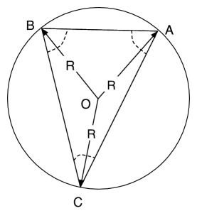
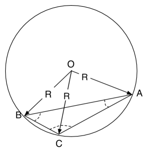
Figure 1: The triangles $T_{A}=\triangle BMC$, $T_{B}=\triangle CMA$, and $T_{C}=\triangle AMB$, in the cases of acute (left) and obtuse (right) triangle

Let $A$, $B$, $C$ be the vertices of the triangle $T$. By the same letters we shall denote the angles corresponding to the vertices of the triangle $T$. Without loss of generality, we may assume that $|AB|={\rm diam}\,T$, and, consequently, $C\geq A$ and $C\geq B$. Let $T_{A}$, $T_{B}$, and $T_{C}$ be triangles obtained by joining the point $M$ with the vertices $A$, $B$ and $C$ (see Figure 1).

Set

$$m(A):=\int\!\!\!\int\limits_{T_{A}}(R^{2}-x^{2}-y^{2})^{p}\,dx\,dy,$$

$$m(B):=\int\!\!\!\int\limits_{T_{B}}(R^{2}-x^{2}-y^{2})^{p}\,dx\,dy,$$

$$m(C):=\int\!\!\!\int\limits_{T_{C}}(R^{2}-x^{2}-y^{2})^{p}\,dx\,dy.$$

Note that in the case of non-obtuse triangles

$$d^{p}(\overline{Q},T,L_{p})=m(A)+m(B)+m(C),$$

and for obtuse triangles ($C>\frac{\pi}{2}$) we have

$$d^{p}(\overline{Q},T,L_{p})=m(A)+m(B)-m(\pi-C).$$

Let the triangle $T_{A}^{1}$ be homothetic to the triangle $T_{A}$ with the side, corresponding to the side $OB$, equal to $1$. From the definition of $m(A)$ it follows that

(27) $$m(A)=\displaystyle R^{2p+2}\int\!\!\!\int\limits_{T_{A}^{1}}(1-x^{2}-y^{2})^{p}\,dx\,dy=\displaystyle 2R^{2p+2}\left(\frac{A}{2p+2}-l(A)\right),$$

where

$$l(A)=\int\limits_{\cos{A}}^{1}x(1-x^{2})^{p}\arccos{\left(\frac{\cos{A}}{x}\right)}\,dx.$$

Note that $l(0)=0$, $l(\pi/2)=\displaystyle\frac{\pi}{4p+4}$ and

$$l^{\prime}(A)=\gamma(p)(\sin{A})^{2p+2},$$

where $\gamma(p)=\frac{1}{2}B\left(p+1,\,\frac{1}{2}\right)$.

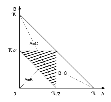
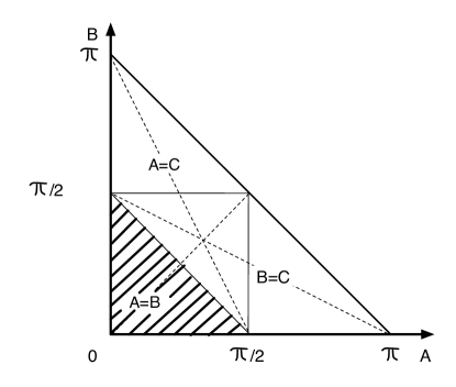
Figure 2: The domains $F_{1}$ (left) and $F_{2}$ (right)

Every triangle with unit area is uniquely determined by the pair of its angles $(A,B)$, which can be considered as the point in the plane with coordinates $(A,B)$. Let $F_{1}$ and $F_{2}$ be the sets of points, which corresponds to the sets of all acute and all obtuse triangles respectively (see Figure 2). Obviously, $F_{1}$ and $F_{2}$ are open sets in the usual topology of $\mathbb{R}^{2}$.

In view of Lemma 10, the infimum in (26) is achieved at some triangle $T_{1}$. Let $A_{1}$, $B_{1}$ and $C_{1}$be the angles of the triangle $T_{1}$.

First, assume that the triangle $T_{1}$ is acute. Taking into account the expression (27), in this case we have

$$d^{p}(\overline{Q},T,L_{p})=m(A)+m(B)+m(C)=2R^{2p+2}\left[\frac{\pi}{2p+2}-l(A)-l(B)-l(C)\right].$$

Since $|T|=1$, we obtain

$$R^{2}=\frac{2}{\sin{2A}+\sin{2B}+\sin{2C}}.$$

Hence,

(28) $$Z(A,B):=\frac{d^{p}(\overline{Q},T,L_{p})}{2^{p+2}}=\displaystyle\frac{\frac{\pi}{2p+2}-l(A)-l(B)-l(C)}{(\sin{2A}+\sin{2B}+\sin{2C})^{p+1}}.$$

Therefore, by the choice of the triangle $T_{1}$,

$$Z(A_{1},B_{1})=\inf_{(A,B)\in F_{1}}Z(A,B).$$

Since $T_{1}$ is an acute triangle, the necessary conditions of extremum have to be satisfied:

(29) $$\begin{array}[]{rclcl}\displaystyle\frac{\partial Z}{\partial A}&=&\left\{\displaystyle\frac{l^{\prime}(C)-l^{\prime}(A)}{(\sin{2A}+\sin{2B}+\sin{2C})^{p+1}}\right.&&\\[12.0pt] &&\;\;-\;\;\left.\left.\displaystyle\frac{(2p+2)(\cos{2A}-\cos{2C})\left[\frac{\pi}{2p+2}-l(A)-l(B)-l(C)\right]}{(\sin{2A}+\sin{2B}+\sin{2C})^{p+2}}\right\}\right|_{{A=A_{1}\atop B=B_{1}}}&=&0\end{array}$$

and

(30) $$\begin{array}[]{rclcl}\displaystyle\frac{\partial Z}{\partial B}&=&\left\{\displaystyle\frac{l^{\prime}(C)-l^{\prime}(B)}{(\sin{2A}+\sin{2B}+\sin{2C})^{p+1}}\right.&&\\[12.0pt] &&\;\;-\;\;\left.\left.\displaystyle\frac{(2p+2)(\cos{2B}-\cos{2C})\left[\frac{\pi}{2p+2}-l(A)-l(B)-l(C)\right]}{(\sin{2A}+\sin{2B}+\sin{2C})^{p+2}}\right\}\right|_{{A=A_{1}\atop B=B_{1}}}&=&0\end{array}$$

From equations (29) – (30) we derive that either the angle $C_{1}$ is equal to one of the other angles of the triangle $T_{1}$ ($C_{1}=A_{1}$ or $C_{1}=B_{1}$) or

$$\frac{l^{\prime}(C_{1})-l^{\prime}(A_{1})}{(\sin{C_{1}})^{2}-(\sin{A_{1}})^{2}}=\frac{l^{\prime}(C_{1})-l^{\prime}(B_{1})}{(\sin{C_{1}})^{2}-(\sin{B_{1}})^{2}}.$$

From the last equation with the help of the expression for $l^{\prime}(A)$ we have:

$$\frac{(\sin{C_{1}})^{2p+2}-(\sin{A_{1}})^{2p+2}}{(\sin{C_{1}})^{2}-(\sin{A_{1}})^{2}}=\frac{(\sin{C_{1}})^{2p+2}-(\sin{B_{1}})^{2p+2}}{(\sin{C_{1}})^{2}-(\sin{B_{1}})^{2}}$$

which can be true only if $A_{1}=B_{1}$. Therefore, if $T_{1}$ is acute then it is isosceles.

Now, if we assume that $T_{1}$ is obtuse then we similarly obtain that $T_{1}$ should be isosceles. Therefore, the triangle $T_{1}$ solving (26) must be either right or isosceles.

Now let us consider the case of right triangles. Then $C=\frac{\pi}{2}$. We shall show that the triangle solving the problem

$$d(\overline{Q},T,L_{p})\to\inf,\quad|T|=1,\;C=\frac{\pi}{2},$$

is isosceles. Indeed, in this case $B=\frac{\pi}{2}-A$ and

$$d^{p}(\overline{Q},T,L_{p})=m(A)+m\left(\frac{\pi}{2}-A\right)+m\left(\frac{\pi}{2}\right)=2\cdot\displaystyle\frac{\displaystyle\frac{\pi}{4p+4}-l(A)-l\left(\frac{\pi}{2}-A\right)}{(\sin{2A})^{p+1}}.$$

Lemma 11

The function

(31) $$L(A):=\displaystyle\frac{\displaystyle\frac{\pi}{4p+4}-l(A)-l\left(\frac{\pi}{2}-A\right)}{(\sin{2A})^{p+1}}$$

is non-increasing on the interval $(0,\pi/4]$.

Proof. Let us consider the derivative of the function $L$:

$$L^{\prime}(A)=\frac{[l^{\prime}(\pi/2-A)-l^{\prime}(A)]\sin{2A}-(2p+2)\cos{2A}\left[\displaystyle\frac{\pi}{4p+4}-l(A)-l(\pi/2-A)\right]}{(\sin{2A})^{p+2}}.$$

Taking into account the expression for $l^{\prime}(A)$, in order to show that $L^{\prime}(A)\leq 0$ on the interval $(0,\pi/4)$ it suffices to prove that

$$r(A):=\gamma(p)[(\cos{A})^{2p+2}-(\sin{A})^{2p+2}]\tan{2A}-(2p+2)\left[\frac{\pi}{4p+4}-l(A)-l(\pi/2-A)\right]\leq 0$$

on the interval $A\in(0,\pi/4)$.

Let us consider the derivative $r^{\prime}(A)$:

$$\begin{array}[]{rcl}r^{\prime}(A)&=&\gamma(p)\Big{\{}\displaystyle\frac{2}{(\cos{2A})^{2}}[(\cos{A})^{2p+2}-(\sin{A})^{2p+2}]\\[12.0pt] &&\begin{array}[]{ll}\quad\quad\;-&(2p+2){\tan}\,2A\sin{A}\cos{A}[(\sin{A})^{2p}+(\cos{A})^{2p}]\\[7.0pt] \quad\quad\;-&(2p+2)[(\cos{A})^{2p+2}-(\sin{A})^{2p+2}]\Big{\}},\end{array}\end{array}$$

where $\gamma(p)=\frac{1}{2}B\left(p+1,\,\frac{1}{2}\right)$.

Set $t={\rm tan}\,A$, and then $t\in(0,1]$. Obviously,

$$r^{\prime}(A)=\frac{\gamma(p)z(t)}{(\cos{A})^{2p+2}},$$

where

$$z(t)=pt^{2p+6}-2t^{2p+4}-(p+2)t^{2p+2}+(p+2)t^{4}+2t^{2}-p.$$

To prove that $r^{\prime}(A)\leq 0$ for all $A\in\left(0,\frac{\pi}{4}\right]$ we shall need the following proposition.

Proposition 1. Let $p\in(0,1)$. Then the function

$$z(t)=pt^{2p+6}-2t^{2p+4}-(p+2)t^{2p+2}+(p+2)t^{4}+2t^{2}-p$$

is non-positive for all $t\in[0,1]$.

Thus, we obtain that $r^{\prime}(A)\leq 0$ for all $A\in\displaystyle\left(0,\frac{\pi}{4}\right]$. Consequently, the function $r(A)$ is non-increasing, and hence $r(A)\leq r(+0)=0$. Hence, we have proved that the function $L(A)$ is non-increasing on the interval $(0,\pi/4]$, i.e.

$$L(A)\geq L(\pi/4)$$

for all $A\in(0,\pi/4)$. $\square$

Note that it can be shown similarly that the function $L(A)$ (see (31)) is non-decreasing on the interval $\displaystyle\left[\frac{\pi}{4},\frac{\pi}{2}\right)$. Therefore,

$$\inf\limits_{|T|=1,\,C=\frac{\pi}{2}}d(\overline{Q},T,L_{p})=d(\overline{Q},T_{2},L_{p}),$$

where $T_{2}$ is the isosceles right triangle.

Hence, we have proved that the triangle $T_{1}$ must be isosceles. Without loss of generality we may assume that $A=B$. Let us show that $T_{1}$ is equilateral. To this end let us consider the following problem

(32) $$d(\overline{Q},T,L_{p})\to\inf,\quad|T|=1,\;A=B.$$

Let us consider now the case when the triangle $T$ is isosceles non-obtuse triangle. Then $A\in\displaystyle\left[\frac{\pi}{4},\frac{\pi}{2}\right)$, and

$$d^{p}(\overline{Q},T,L_{p})=2m(A)+m(\pi-2A)=2^{p+2}\cdot\displaystyle\frac{\frac{\pi}{2p+2}-2l(A)-l(\pi-2A)}{(2\sin{2A}-\sin{4A})^{p+1}}.$$

Lemma 12

The function

$$S(A)=\displaystyle\frac{\frac{\pi}{2p+2}-2l(A)-l(\pi-2A)}{(2\sin{2A}-\sin{4A})^{p+1}}$$

is non-increasing for $A\in[\pi/4,\pi/3]$ and is non-decreasing for $A\in[\pi/3,\pi/2)$.

Proof. Let us consider the derivative of the function $S$

(33) $$\begin{array}[]{rcl}S^{\prime}(A)&=&\displaystyle\frac{8\cos{A}(\sin{A})^{3}[2l^{\prime}(\pi-2A)-2l^{\prime}(A)]}{(8\cos{A}(\sin{A})^{3})^{p+2}}\\[12.0pt] &&\;\;-\;\;\displaystyle\frac{8(p+1)\sin{A}\sin{3A}\left[\frac{\pi}{2p+2}-2l(A)-l(\pi-2A)\right]}{(8\cos{A}(\sin{A})^{3})^{p+2}}.\end{array}$$

Obviously, the denominator of the right hand side of (33) is positive in the considered region. In what follows we shall consider only the numerator of  (33). Then showing that $S^{\prime}(A)\leq 0$, when $A\in[\pi/4,\pi/3]$ and $S^{\prime}(A)\geq 0$ when $A\in[\pi/3,\pi/2)$, is equivalent to proving the inequality:

$$\begin{array}[]{rcl}q(A)&:=&2\gamma(p)\displaystyle\frac{\cos{A}\sin{A}}{3-4(\sin{A})^{2}}\Big{[}(\sin{2A})^{2p+2}-(\sin{A})^{2p+2}\Big{]}\\[12.0pt] &&\;\;-\;\;(p+1)\left[\displaystyle\frac{\pi}{2p+2}-2l(A)-l(\pi-2A)\right]\leq 0\end{array}$$

for all $A\in[\pi/4,\pi/2)$.

It is easy to see that $q(\pi/2-0)=0$ and

$$\begin{array}[]{rcl}q^{\prime}(A)&=&\displaystyle\frac{2\gamma(p)}{\left[3-4(\sin{A})^{2}\right]^{2}}\Big{\{}\left[(\sin{2A})^{2p+2}-(\sin{A})^{2p+2}\right]\\[7.0pt] &&\begin{array}[]{ll}\qquad\qquad\qquad\qquad\times&\Big{[}\cos{2A}\Big{(}3-4(\sin{A})^{2}\Big{)}+8(\cos{A})^{2}(\sin{A})^{2}\\[7.0pt] &\;\;-\;\;(p+1)\Big{(}3-4(\sin{A})^{2}\Big{)}^{2}\Big{]}\\[7.0pt] \qquad\qquad\qquad\qquad+&2(p+1)\cos{A}\sin{A}\Big{[}3-4(\sin{A})^{2}\Big{]}\\[7.0pt] &\;\;\times\;\;\left[2\cos{2A}(\sin{2A})^{2p+1}-\cos{A}(\sin{A})^{2p+1}\right]\Big{\}}.\end{array}\end{array}$$

Obviously,

$$q^{\prime}(A)=\frac{\gamma(p)}{\left[3-4(\sin{A})^{2}\right]^{2}}z(t),\quad t=2\cos{A}\in(0,\sqrt{2}],$$

where

$$\begin{array}[]{rcl}z(t)&:=&(t^{2p+2}-1)\cdot\Big{[}(t^{2}-2)(t^{2}-1)+t^{2}(4-t^{2})-2(p+1)(t^{2}-1)^{2}\Big{]}\\[7.0pt] &&\qquad\qquad\qquad\;\;+\;\;(p+1)t(t^{2}-1)\Big{[}2(t^{2}-2)t^{2p+1}-t\Big{]}\\[7.0pt] &=&-(2p+1)t^{2p+4}+2(p+2)t^{2p+2}+(p+1)t^{4}-(3p+4)t^{2}+2p.\end{array}$$

We shall need the following proposition to show that $z(t)$ changes its sign exactly once.

Proposition 2. Let $p\in(0,1)$. Then the function

$$z(t)=-(2p+1)t^{2p+4}+2(p+2)t^{2p+2}+(p+1)t^{4}-(3p+4)t^{2}+2p$$

has exactly one point of sign change (from positive to negative) on the segment $[0,2]$, and this point is located inside the interval $(0,1)$.

Therefore, $z(t)$ changes its sign on the segment $[0,\sqrt{2}]$ exactly once from positive to negative. Since variable $A$ increases when variable $t$ decreases, the function $q^{\prime}(A)$ changes sign exactly once as well, from negative to positive. Hence,

$$q(A)\leq\min\left\{q(\pi/4);\,q(\pi/2-0)\right\}=0,$$

whenever $q(\pi/4)=\gamma(p)(1-2^{-p-1})-(p+1)\left[\frac{\pi}{4p+4}-2l(\pi/4)\right]\leq 0$ (this will be shown in the proof of Lemma 13). Hence, we have proved that $S^{\prime}(A)\leq 0$ for $A\in[\pi/4,\pi/3]$, and $S^{\prime}(A)\geq 0$ for $A\in[\pi/3,\pi/2)$. $\square$

Let us turn now to the case of isosceles obtuse triangles $T$. In this case $A\in\left(0,\frac{\pi}{4}\right)$, and

$$d^{p}(\overline{Q},T,L_{p})=2m(A)-m(2A)=2^{p+2}\cdot\displaystyle\frac{-2l(A)+l(2A)}{(2\sin{2A}-\sin{4A})^{p+1}}.$$

Lemma 13

The function

$${\widetilde{S}}(A)=\displaystyle\frac{-2l(A)+l(2A)}{(2\sin{2A}-\sin{4A})^{p+1}}$$

is non-increasing on the interval $\left(0,\frac{\pi}{4}\right]$.

Proof. Let us consider the derivative of the function $\widetilde{S}$

$$\begin{array}[]{rcl}{\widetilde{S}}^{\prime}(A)&=&\displaystyle\frac{8\cos{A}(\sin{A})^{3}[2l^{\prime}(2A)-2l^{\prime}(A)]}{(8\cos{A}(\sin{A})^{3})^{p+2}}\\[12.0pt] &&\;\;-\;\;\displaystyle\frac{8(p+1)\sin{A}\sin{3A}[-2l(A)+l(2A)]}{(8\cos{A}(\sin{A})^{3})^{p+2}}.\end{array}$$

We shall show that ${\widetilde{S}}^{\prime}(A)\leq 0$ when $A\in(0,\,\pi/4]$ or, equivalently, that ${\tilde{q}}(A)\leq 0$ for all $A\in(0,\,\pi/4]$ where

$$\begin{array}[]{rcl}{\tilde{q}}(A)&:=&2\gamma(p)\displaystyle\frac{\cos{A}\sin{A}}{3-4(\sin{A})^{2}}\Big{[}(\sin{2A})^{2p+2}-(\sin{A})^{2p+2}\Big{]}\\[12.0pt] &&\;\;-\;\;(p+1)[-2l(A)+l(2A)].\end{array}$$

The derivative of ${\tilde{q}}(A)$ can be written as:

$$\begin{array}[]{rcl}{\tilde{q}}^{\prime}(A)&=&\displaystyle\frac{2\gamma(p)}{\left[3-4(\sin{A})^{2}\right]^{2}}\Big{\{}\left[(\sin{2A})^{2p+2}-(\sin{A})^{2p+2}\right]\\[7.0pt] &&\begin{array}[]{ll}\qquad\qquad\qquad\quad\times&\Big{[}\cos{2A}\Big{(}3-4(\sin{A})^{2}\Big{)}+8(\cos{A})^{2}(\sin{A})^{2}\\[7.0pt] &\;\;-\;\;(p+1)\Big{(}3-4(\sin{A})^{2}\Big{)}^{2}\Big{]}\\[7.0pt] \qquad\qquad\qquad\quad+&2(p+1)\cos{A}\sin{A}\Big{[}3-4(\sin{A})^{2}\Big{]}\\[7.0pt] &\;\;\times\;\;\left[2\cos{2A}(\sin{2A})^{2p+1}-\cos{A}(\sin{A})^{2p+1}\right]\Big{\}}\end{array}\\[7.0pt] &=&\displaystyle\frac{\gamma(p)}{\left[3-4(\sin{A})^{2}\right]^{2}}z(t),\end{array}$$

where $t=2\cos{A}\in[\sqrt{2},\,2)$ and

$$z(t)=-(2p+1)t^{2p+4}+2(p+2)t^{2p+2}+(p+1)t^{4}-(3p+4)t^{2}+2p.$$

In view of Proposition 2, it follows that $z(t)\leq 0$ for all $t\in[\sqrt{2},\,2)$. Hence, ${\tilde{q}}^{\prime}(A)\leq 0$ on the segment $(0,\,\pi/4]$. Therefore, ${\tilde{q}}(A)\leq{\tilde{q}}(+0)=0$ (in particular, $q(\pi/4)={\tilde{q}}(\pi/4)\leq 0$) and ${\tilde{S}}(A)$ is non-increasing on the segment $(0,\,\pi/4]$. $\square$

Combining Lemmas 12 and 13 we conclude that

$$\inf_{|T|=1,\,A=B}d(\overline{Q},T,L_{p})=d(\overline{Q},T_{3},L_{p}),$$

where $T_{3}$ is equilateral triangle. Moreover, $T_{3}$ is the only triangle which solves (32). Since the triangle $T_{1}$ solves (26) and is isosceles, we obtain that $T_{1}=T_{3}$, which finishes the proof.

Department of Mathematical Analysis
Dnepropetrovsk National University
Institute of Applied Mathematics and Mechanics of NAS of Ukraine
pr. Gagarina, 72,
Dnepropetrovsk, UKRAINE, 49050
Phone: +380567609461
Email: babenko.vladislav@gmail.com

Department of Mathematics and Statistics
Sam Houston State University
Box 2206
Huntsville, TX, USA 77340-2206
Phone: 936.294.4884
Fax: 936.294.1882
Email: babenko@shsu.edu

Department of Mathematical Analysis
Dnepropetrovsk National University
pr. Gagarina, 72
Dnepropetrovsk, UKRAINE, 49050
Email: dmitriy.skorokhodov@gmail.com

References

[1]
V. Babenko, Yu. Babenko, A. Ligun, A. Shumeiko, On asymptotical behavior of the optimal linear spline
interpolation error of functions, East J. Approx., V. 12, N. 1 (2006), 71–101.
[2]
Yu. Babenko, On the asymptotic behavior of the optimal error of spline interpolation of multivariate functions, PhD thesis, 2006.
[3]
K. Brczky, Approximation of general smooth convex bodies, Adv. in Math.,
153 (2000) 325–341.
[4]
K. Brczky, M. Ludwig, Approximation of Convex Bodies and a Momentum Lemma
for Power Diagrams, Monatshefte fr Mathematik, V. 127, N. 2, (1999) 101–110.
[5]
L. Chen, P. Sun, J. Xu Optimal anisotropic meshes for minimizing interpolation errors in -norm,
Math. Comp.,
[6]
E. F. D’Azevedo, R. B. Simpson, On optimal interpolation triangle incidences. SIAM J. Sci. Statist.
Comput. 10 (1989), no. 6, 1063–1075.
[7]
L. Fejes Toth, Lagerungen in der Ebene, auf der Kugel und im Raum, 2nd edn. Berlin: Springer, 1972.
[8]
P. Gruber, Volume approximation of convex bodies by inscribed polytopes, Math. Ann., V. 281, 1988,
pp.229–245.
[9]
E. Nadler, Piecewise linear best approximation on triangles, in: Chui, C.K., Schumaker, L.L. and
Ward, J.D. (Eds.), Approximation Theory V, Academic Press, (1986) 499–502.
[10]
H. Pottmann, R. Krasauskas, B. Hamann, K. Joy, W. Seibold, On piecewise linear approximation of quadratic
functions, J. Geom. Graph. 4, no. 1, (2000) 31–53.