Impact of background flow on dissolution trapping of carbon dioxide injected into saline aquifers

Abstract.

While there has been a large interest in studying the role of dissolution-driven free convection in the context of geological sequestration, the contribution of forced convection has been largely ignored. This manuscript considers CO₂ sequestration in saline aquifers with natural background flow and uses theoretical arguments to compute the critical background velocity needed to establish the forced convective regime. The theoretical arguments are supported by two dimensional high-resolution numerical simulations which demonstrate the importance of forced convection in enhancing dissolution in aquifers characterised by low Rayleigh numbers.

1. Introduction

Geological storage of carbon dioxide in deep saline aquifers is considered to be one of the key technological solutions to mitigating carbon emissions in the near future (IPCC (2005)). Under the thermodynamic conditions at which CO₂ is injected into subsurface formations, CO₂ exists in a supercritical state with a density that is lower than that of brine in the medium. Due to this difference in density, CO₂ rises to the top of the domain and containment is achieved by the presence of an overlying low-permeability caprock.

Due to the tremendous importance of understanding the processes leading to storage security of injected carbon dioxide, there has been a large body of published literature exploring the different trapping mechanisms. The physical processes that play a role at increasing timescales are $(i)$ physical trapping due to the caprock, $(ii)$ residual trapping of bubbles of CO₂ in the porous rock, $(iii)$ dissolution trapping due to the slow dissolution of CO₂ into the brine and $(iv)$ mineral trapping due to chemical reactions between dissoved carbon dioxide and host rocks. The work presented in this manuscript is concerned with dissolution trapping mechanism under different aquifer flow conditions. Experimental data has shown that the dissolution of CO₂ into brine produces a weak density contrast, with CO₂ saturated brine being slightly denser than unsaturated brine. Most recent work in this area has focused on the free convective mixing that can arise due to this difference in density.

One of the effects that has so far been neglected is the contribution of background flow to the rate of dissolution of CO₂ into the brine in the aquifer. The only exception we are aware of is the work by Hassanzadeh et al. (2009), where the authors have analysed the role of additional dispersion due to the background flow. For a finite sized CO₂ plume in the supercritical state, the background flow leads to the development of a boundary layer in which horizontal advection balances the diffusion of dissolved carbon dioxide. We will henceforth refer to the dissolution occuring due to the background flow as forced convection. A compilation of reservoir characteristics for potential sites in western Canada by Bachu et al. (2004) suggests that the Rayleigh numbers are going to be fairly low for a large number of storage sites. Recent computations (Rapaka et al. (2008)) as well as experiments (Backhaus et al. (2011)) in analogous systems have shown that the free convective mechanism (fingering) can take very long to establish under such conditions. It is possible that forced convection can play the dominant role in enhancing storage security in this scanario. However, in the context of geological storage of carbon dioxide, the conditions under which forced convection is the preferred state have not yet been explored. In this manuscript, we will provide simple theoretical arguments for the background flow conditions under which forced convection establishes itself and support these predictions with high resolution numerical simulations.

2. Governing Equations and Solution Procedure

We consider the dynamics of CO₂ dissolution and transport in a aquifer of depth $H^{*}$ with an overlying source of CO₂ of length $L^{*}$. We assume the presence of a horizontal background aquifer flow $\mathbf{u}^{*}_{0}=(u^{*}_{0},0)$, the magnitude of which determines whether the system is in a free or forced convective regime.

The equations needed to describe the system are those describing conservation of mass, momentum (Darcy’s law) and an advection-diffusion equation for the concentration of dissolved CO₂. Experimental data has shown that the density of brine increases linearly with the concentration of dissolved CO₂, with a maximum increase (under saturated conditions) of the order of 1% (Pruess and Spycher (2006)). Hence, we utilize the Boussinesq model, where the density of brine is taken to be a constant everywhere except in the buoyancy term. The governing equations are:

$$\frac{\mu^{*}}{k^{*}}\mathbf{u}^{*} =-\nabla^{*}P^{*}+\rho_{f}^{*}g\mathbf{e}_{y},$$ (1)

$$\nabla^{*}\cdot\mathbf{u}^{*} =0,$$ (2)

$$\frac{\partial(\phi C^{*})}{\partial t^{*}}+\nabla^{*}\cdot\left(\mathbf{u}^{*}C^{*}\right) =\nabla^{*}\cdot\phi D^{*}\nabla^{*}C^{*},$$ (3)

$$\rho_{f}^{*} =\rho_{0}^{*}+\Delta\rho^{*}\left(\frac{C^{*}}{C_{0}^{*}}\right),$$ (4)

where, $\mathbf{u}^{*}=\left(u^{*},v^{*}\right)$ is the velocity of the fluid, $C^{*}$ is the concentration of dissolved carbon dioxide, $P^{*}$ is the fluid pressure, $g$ is the acceleration due to gravity, $k^{*}$ is the permeability of the rock, $\rho_{0}^{*}$ is the density of unsaturated brine, $\Delta\rho^{*}$ is the density difference between brine saturated with CO₂ and pure brine, $\mu^{*}$ is the viscosity of brine, $\phi$ is the porosity of the medium and $D^{*}$ is the diffusivity of CO₂ in brine.

We now non-dimensionalize the equations choosing a convective velocity scale $U_{r}=k^{*}\Delta\rho^{*}g/\mu^{*}$, the system depth as a length scale $L_{r}=H^{*}$, and a convective time scale $T_{r}=L_{r}/U_{r}$. Concentrations are non-dimensionalized using $C_{0}^{*}$, the maximum solubility of CO₂ in brine at the conditions in the aquifer. The non-dimensional equations obtained are:

$$\mathbf{u} =-\nabla P+C\mathbf{e}_{y}$$ (5)

$$\nabla\cdot\mathbf{u} =0$$ (6)

$$\frac{\partial C}{\partial t}+\nabla\cdot\left(\mathbf{u}C\right) =\frac{1}{Ra}\nabla^{2}C$$ (7)

The non-dimensional paramerer $Ra$ is the ratio of the convective flux to the diffusive one:

$$Ra =\frac{k^{*}\Delta\rho^{*}gH^{*}}{\mu^{*}\phi D^{*}}$$ (8)

The initial conditions are given by $C=0,u=u_{0}$ and $v=0$ everywhere. The CO₂ concentration is fixed on the top boundary to be $C=1$ for a source region of length $L$, and a no-flux boundary condition is applied for the remainder of the top boundary and the entire bottom boudary. On the left boundary, we have $C=0,u=u_{0}$ and $v=0$ and an outflow boundary condition is applied on the right boundary. A schematic of the geometry considered is shown in Fig. (1).

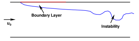
Figure 1. Schematic illustration of the problem geometry considered in this manuscript. The red part of the top boundary denotes the footprint of CO₂ plume in supercritical state. A mean horizontal flow of magnitude $u_{0}$ is taken to be flowing through the system.

Depending on the magnitude of the background flow $u_{0}$, CO₂ dissolution can be enhanced by free convection (low $u_{0}$, sufficiently high $Ra$), forced convection (high $u_{0}$) or be a purely diffusion-driven process (low $u_{0}$, low $Ra$). The case of free convection (especially in the absence of any background flow) has received a great amount of attention in the recent past (see for instance Ennis-King et al. (2005), Xu et al. (2006), Riaz et al. (2006), Hassanzadeh et al. (2007), Rapaka et al. (2008) and Slim and Ramakrishnan (2010)). There is an extensive body of published research on forced convection in porous media over the last four decades, and it is not possible to present present an overview of even the most important contributions within the scope of this paper. The reader is referred to the book by Nield and Bejan (2006) where a comprehensive account of the existing body of work is presented. However, in the context of geological storage of carbon dioxide, we are not aware of any manuscript that points out the conditions under which forced convection plays a dominant role in enhancing the dissolution of injected CO₂. For sufficiently large background flow rates, we expect to see a forced convective regime achieving a steady-state dissolution rate. Using the commonly made assumption of $\frac{\partial^{2}C}{\partial x^{2}}<<\frac{\partial^{2}C}{\partial y^{2}}$ in the boundary layer and assuming that the basic velocity field is of the form $u=u_{0},v=0$, the steady state advection diffusion equation can be reduced to:

$$u_{0}\frac{\partial C}{\partial x} =\frac{1}{Ra}\frac{\partial^{2}C}{\partial y^{2}}$$ (9)

Looking for similarity solutions of the form $1-C(x,y)=f(\xi)$ in terms of the similarity variable $\xi=y/\sqrt{x}$, it is easy to show that $f(\xi)$ satisfies the following differential equation:

$$f^{\prime\prime}+\frac{1}{2}Rau_{0}f^{\prime}\xi=0$$ (10)

where, primes denote differentiation with respect to the similarity variable. The solution of this equation can be shown to be:

$$f(\xi) =erf(\xi\sqrt{Rau_{0}}/2)$$ (11)

giving the dissolution rate at the top boundary as

$$-\frac{\partial C}{\partial y}(y=0) =\frac{\sqrt{Rau_{0}}}{2\sqrt{x}}.$$ (12)

Integrating this expression from $x=0$ to $L$, we get the total dissolution rate to be $Nu=\sqrt{Rau_{0}L}=\sqrt{Pe}$, where $Pe=u_{0}L^{*}/\phi D$ is the Peclet number based on the size of the CO₂ plume.

It can be seen that the total dissolution rate under conditions of forced convection scales with the length of the plume as $\sqrt{L}$. In the free convection regime however, the total dissolution rate scales linearly with $L$. We expect the presence of a critical velocity $u_{c}(L)$ such that, for slow background flows characterized by $u_{0}<u_{c}(L)$, the system will be in a state of free (mixed) convection, whereas for $u_{0}>u_{c}(L)$, we will transition to the forced convection regime.

To determine the critical background flow velocity $u_{c}(L)$, we need an expression for the mean dissolution rate as a function of Rayleigh number under free convective conditions. Recent studies have looked at the time-averaged Nusselt number under free convective conditions and proposed scalings of the form $Nu\sim Ra^{\alpha}$. Neufeld et al. (2010) have used scaling arguments and experiments to suggest $\alpha=0.8$, while Backhaus et al. (2011) have used experiments to obtain a best-fit exponent of $\alpha=0.76$. However, the experiments by both authors were performed under conditions of very high Rayleigh numbers, of the order of $10^{4}$ or higher. In this study, we will use a simpler model given by

$$Nu=\frac{RaL}{40}$$ (13)

which is the well-known relation between Nusselt number and Rayleigh numbers for steady convection when $Ra$ is close to the critical Rayleigh number (Elder (1967)). This relation is known to overpredict the Nusselt number for large $Ra$, but is in good agreement with experimental data for $Ra<250$. Since the focus of this manuscript is on aquifers with lower permeabilities, we use this relation as a useful approximation whose accuracy will be examined a posteriori. Requiring the free and forced convective fluxes to agree at $u_{0}=u_{c}(L)$, we get

$$u_{c}(L) =\frac{RaL}{1600}.$$ (14)

We now look at some values for the parameters characteristic of real formations. We use data from Bachu et al. (2004), where a vast amount of information about the potential sites in western Canada is presented. Using the data from Pruess and Spycher (2006), we estimate the density increase $\Delta\rho^{*}$ to be $5kg/m^{3}$ (corresponding to a salt mass fraction of 0.1). Assuming $k^{*}=10mD,g=10m/s^{2},H^{*}=50m,\mu^{*}=0.5mPa.s,\phi=0.2$ and $D^{*}=1\times 10^{-9}$, we get the Rayleigh number to be $Ra=250$. The convective velocity scale is $U_{r}=k^{*}\Delta\rho^{*}g/\mu^{*}=3cm/year.$ Assuming a CO₂ plume size of $2km$, we can compute the critical background flow velocity needed to transition to a forced convective regime as $u_{c}^{*}=20cm/year$ (where the asterisk denotes dimensional quantity).

2.1. Computational Method

To investigate the transition from free to forced convective flow, we developed a highly efficient solver for the governing equations. The numerical solution of forced convection problems becomes computationally very expensive due to the large linear systems which need to be solved for the velocity field. We have overcome this difficulty by using an eigenfunction expansion in the vertical direction using a Fourier sine series.

The equations to be solved are Eqns.(5-7) subject to the initial and boundary conditions mentioned above. The velocity field is solved obtained using a streamfunction formulation, where the streamfunction $\psi$ is defined using the relation $\mathbf{u}=\nabla\times\psi\mathbf{e}_{z}$. Applying the curl operator to Eqn. (5), we get the following Poisson equation for the velocity field:

$$\nabla^{2}\psi =-\frac{\partial C}{\partial x}$$ (15)

The boundary conditions are given by $\psi=0$ at $y=0$, $\psi=u_{0}$ at $y=1$, $\psi=u_{0}y$ along the left boundary and $\partial\psi/\partial x=0$ along the outflow boundary. We now expand the streamfunction in a Fourier sine-expansion in the vertical direction as:

$$\psi(x,y) =u_{0}y+\sum_{n=1}^{N}\widehat{\psi}_{n}(x)sin(n\pi y)$$ (16)

Substituting this expansion in Eqn. (15) followed by a multiplication with $sin(m\pi y)$ and integration in the vertical direction, we get:

$$\frac{d^{2}\widehat{\psi}_{m}}{dx^{2}}-n^{2}\pi^{2}\widehat{\psi}_{m} =-2\int_{0}^{1}\frac{\partial C}{\partial x}sin(m\pi y)dy$$ (17)

This solution method depends crucially on a theorem about Fourier transforms which guarantees convergence of the term-by-term integral of a Fourier series, even if the original series is divergent (see Theorem 9.8.1 from Prosperetti (2011)). This issue is important to consider since the integrand $\frac{\partial C}{\partial x}$ may not necessarily vanish at the boundaries.

Eqn. (17) is now a set of $N_{y}$ ordinary differential equations in the horizontal direction, where $N_{y}$ is the number of vertical grid-points. These equations can be discretised using the standard second-order finite difference method, resulting in a set of tridiagonal equations that can be solved efficiently. Once the velocity field is obtained from the streamfunction, the concentration field is updated using a second order explicit Adams-Bashforth method. During the very first time step, we use a second order Runge-Kutte method for advancing the concentration solution.

The simulations are performed using 128 uniformly spaced nodes in the vertical direction and $L\times 128$ uniformly spaced nodes in the horizontal direction. The variables are located on the grid in a staggered fashion, with concentrations evaluated at the center of the cells and velocities evaluated on the faces. The streamfunction is defined at the top-right corner of each cell. We use constant intervals for timestepping, with a nondimensional timestep of $\Delta t=10^{-4}$, chosen to satisfy both the diffusive stability condition $\frac{1}{Ra}\frac{\Delta t}{\Delta x^{2}}<\frac{1}{2}$ and the Courant-Friedrichs-Levy condition $\frac{u_{0}\Delta t}{\Delta x}<1$ (Ferziger and Peric (2001)).

3. Results

We have used the computational technique described above to investigate the transition from free to forced convection for $Ra=50,100,200$ and $400$, and for $u_{0}$ varying between $0.1$ and $10.0$. The length of the CO₂ source was varied between $L=10$ to $L=40$. In Fig. (3), we plot the Nusselt numbers computed for the simulations scaled with $RaL$, where the Nusselt number is defined as:

$$Nu =\int_{x=0}^{L}-\frac{\partial C}{\partial y}(y=0)dx$$ (18)

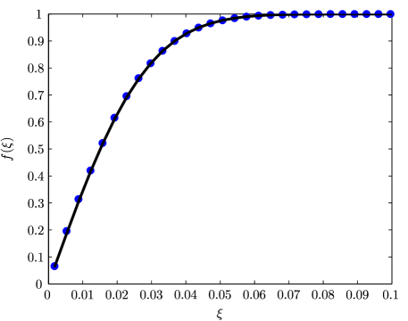
Figure 2. Comparison between the theoretically predicted concentration profile $C(x,y)=1-erf(y\sqrt{Rau_{0}}/2\sqrt{x})$ (black line) and that computed from a simulation (blue symbols)) with $Ra=400,u_{0}=10$ along a line at the center of the CO₂ source.

We first verify that the grid spacing used in the simulations is fine enough to resolve the boundary layer by performing a simulation with $Ra=400$ and $u_{0}=10$ ( the highest values for both parameters considered in this manuscript). We compare the profile of dissolved carbon dioxide in the vertical direction at the center of the plate with the similarity solution given by Eqn. (11). In Fig. (2), we plot the computed boundary layer profile using blue symbols and the analytical solution using the black line. The simulations are seen to match the theoretical solution well, confirming that the resolution is fine enough to resolve the boundary phenomena.

From the scaling arguments presented in the previous section, $Nu/RaL=1/40$ in the free convection regime for low Rayleigh numbers and $Nu/RaL=\sqrt{u_{0}/RaL}$ in the forced convective regime. These scalings are plotted using dashed lines in Fig. (3). It must be noted that the parameter combination $RaL$ that occurs in the analysis is a Rayleigh-number that is based on choosing the size of the CO₂ source as a length scale instead of the depth of the medium. The simulations are performed upto time $T=10$ and the Nusselt number is computed by averaging the instantaneous values from $t=9.5$ to $t=10$, and these average values are plotted using blue circles. It can be seen that both the computed Nusselt numbers and the critical velocity agree very well with those predicted using theoretical arguments.

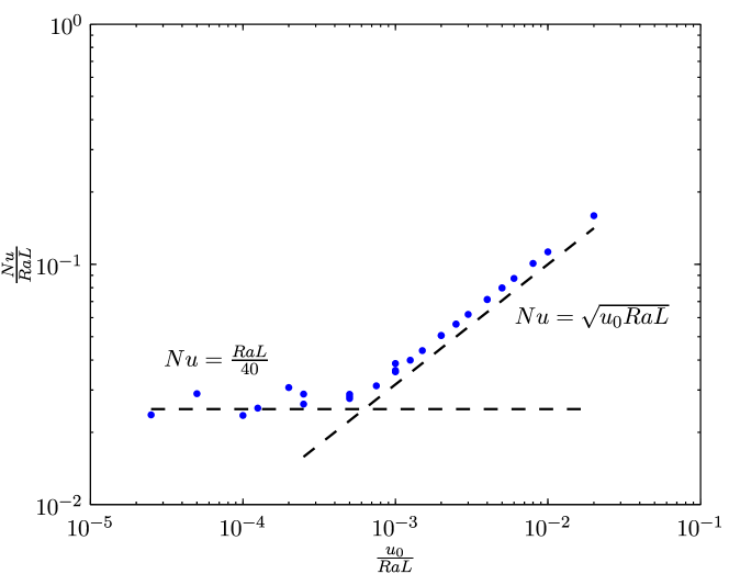
Figure 3. Comparison of scaled Nusselt number, $\frac{Nu}{RaL}$ computed from simulations (blue circles) and the theoretical predictions for free and forced convective regimes (dashed lines) for different background flow rates, scaled as $\frac{u_{0}}{RaL}$

For concreteness, we present contours of the dissolved concentration of CO₂ for simulations fixed with $Ra=400$ and $L=10$ in Fig. (4) for background flow velocities of $u_{0}=1,2,3,4,5$ and $10$. The predicted critical velocity for transition to forced convection is $u_{c}=2.5$. The contours show instantaneoous snapshots of the system at $t=10$. It is seen that for velocities $u_{0}>u_{c}$, the flow resembles forced convective behavior closely. Also presented in Fig. (5) are the computed $Nu/RaL$ at different times for this problem with $u_{0}=2$ (blue line) and $u_{0}=3$ (black line). The simulation with $u_{0}=2$ is slightly below the critical velocity and demonstrates free-convective behavior which can be identified using the distinct minima in the dissolution rate followed by an enhancement due to the effect of fingering. The case with $u_{0}=3$ on the other hand achieves a steady state dissolution rate and does not display the minima. The dashed lines represent average Nusselt numbers that were used in Fig. (4). The fluctuations in the Nusselt number are due to the fact that the simulations are continuously forced (once every 100$\Delta t$), to produce fingering phenomena when that is the preferred state of the system. In the absence of continous forcing, the simulations can reach an artificial steady state even when fingering is the preferred state after the initial perturbations have been flushed out of the domain by the background flow.

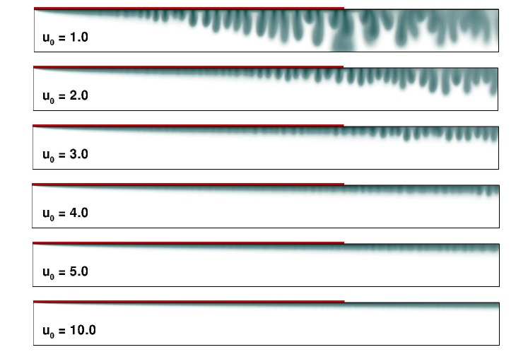
Figure 4. Contours of concentration of dissolved CO₂ for simulations with $Ra=400$ and $L=10$. The predicted critical velocity is $u_{c}=2.5$, beyond which the dynamics near the CO₂ source are predicted to resemble forced convection. The location of the CO₂ source is marked in red.

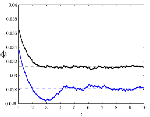
Figure 5. Nusselt number at different times for two simulations with $Ra=400$ and $u_{0}=2.0$ (blue line) and $u_{0}=3.0$ (black line). The critical velocity from theory is $u_{0}=2.5$.

4. Discussion

The results presented in this manuscript describe how the presence of a background flow alters the dynamics of CO₂ dissolution in saline aquifers. The main implications of these results are:

1. An accurate understanding of the magnitude and direction of background flows is needed to locate monitoring wells. In the presence of a reasonably strong background flow, monitoring wells located right under the CO₂ plume to investigate dissolved carbon content might never record fluid with meaningful concentrations of carbon dioxide. In the presence of experimental data on existing background flow conditions, these simulations can be used to suggest suitable locations to place monitoring wells.

2. For low Rayleigh number systems, forced convection can result in far higher dissolution rates than free convection. Further, the magnitude of the rates of dissolution can be estimated quite accurately using the well-known theoretical formulae. Another benefit of the constant dissolution rate due to forced convection has to do with upscaling into larger reservoir simulators where the boundary layer cannot be resolved.

3. In this work, we have not explicitly included the role of either hydrodynamic dispersion, or anisotropy of the permeability tensor. In the context of the simple theoretical arguments presented in this paper, hydrodynamic dispersion essentially serves to define an effective (higher) diffusion coefficient which will push the critical velocity lower and the Nusselt number under conditions of forced convection higher. Similarly, the presence of a permeability anisotropy with higher horizontal permeability will tend to make forced convection even more efficient than suggested in this manuscript.

5. Acknowledgements

This work was supported by the US Department of Energy through the Zero Emissions Research and Technology (ZERT) Project.

References

- Bachu et al. [2004] S. Bachu, J. M. Nordbotten, and M. A. Celia. Evaluation of the spread of acid gas plumes injected in deep saline aquifers in western canada as an analogue to co2 injection in continental sedimentary basins. In D. W. K. E. S. Rubin and C. F. Gilboy, editors, Proceedings of 7th International Conference on Greenhouse Gas Control Technologies, pages 449–457. Elsevier, 2004.
- Backhaus et al. [2011] S. Backhaus, K. Turitsyn, and R. E. Ecke. Convective instability and mass transport of diffusion layers in a hele-shaw geometry. Phys. Rev. Lett., (Submitted), 2011.
- Elder [1967] J. W. Elder. Steady free convection in a porous medium heated from below. J. Fluid Mech., 27:29–48, 1967.
- Ennis-King et al. [2005] J. Ennis-King, I. Preston, and L. Paterson. Onset of convection in anisotropic porous media subject to a rapid change in boundary conditions. Phys. Fluids, 17(8):084107, 2005.
- Ferziger and Peric [2001] J. H. Ferziger and M. Peric. Computational Methods for Fluid Dynamics. Springer, 2001.
- Hassanzadeh et al. [2007] H. Hassanzadeh, P. M. Darvish, and D. W. Keith. Scaling behavior of convective mixing, with application to geological storage of CO2. AIChE J., 53(5):1121–1131, 2007.
- Hassanzadeh et al. [2009] H. Hassanzadeh, M. Pooladi-Darvish, and D. W. Keith. The effect of natural flow of aquifers and associated dispersion on the onset of buoyancy-driven convection in a saturated porous medium. AIChE J., 55(2):475–485, 2009. doi: 10.1002/aic.11664.
- IPCC [2005] IPCC. IPCC Special Report on Carbon Dioxide Capture and Storage. Prepared by Working Group III of the Intergovernmental Panel on Climate Change [B. Metz, O. Davidson, H. C. de Coninck, M. Loos and L. A. Meyer]. Cambridge University Press, 2005.
- Neufeld et al. [2010] J. A. Neufeld, M. A. Hesse, A. Riaz, M. A. Hallworth, H. A. Tchelepi, and H. E. Huppert. Convective dissolution of carbon dioxide in saline aquifers. Geophys. Res. Lett., 37(L22404), 2010.
- Nield and Bejan [2006] D. A. Nield and A. Bejan. Convection in Porous Media. Springer, 3rd edition, 2006.
- Prosperetti [2011] A. Prosperetti. Advanced Mathematics for Applications. Cambride University Press, 2011.
- Pruess and Spycher [2006] K. Pruess and N. Spycher. ECO2N: A new TOUGH2 fluid property module for studies of CO2 storage in saline aquifers. In TOUGH Symposium 2006. Lawrence Berkeley National Laboratory, Berkeley CA, 2006.
- Rapaka et al. [2008] S. Rapaka, S. Chen, R. J. Pawar, P. H. Stauffer, and D. Zhang. Nonmodal growth of perturbations in density-driven convection in porous media. J. Fluid Mech., 609:285–303, 2008.
- Riaz et al. [2006] A. Riaz, M. Hesse, H. A. Tchelepi, and F. M. Orr. Onset of convection in a gravitationally unstable diffusive boundary layer in porous media. Journal of Fluid Mechanics, 548:87–111, 2006.
- Slim and Ramakrishnan [2010] A. Slim and T. S. Ramakrishnan. Onset and cessation of time-dependent, dissolution-driven convection in porous media. Phys. Fluids, 22(124103), 2010.
- Xu et al. [2006] X. Xu, S. Chen, and D. Zhang. Convective stability analysis of the long-term storage of carbon dioxide in deep saline aquifers. Adv. Water Resour., 29:397–407, Mar 2006.