Efficiency for preforming molecules from mixtures of light Fermi and heavy Bose atoms in optical lattices: the strong-coupling-expansion method

Abstract

We discuss the application of a strong-coupling expansion (perturbation theory in the hopping) for studying light-Fermi-heavy-Bose (like ⁴⁰K-⁸⁷Rb) mixtures in optical lattices. We use the strong-coupling method to evaluate the efficiency for pre-forming molecules, the entropy per particle and the thermal fluctuations. We show that within the strong interaction regime (and at high temperature), the strong-coupling expansion is an economical way to study this problem. In some cases, it remains valid even down to low temperatures. Because the computational effort is minimal, the strong-coupling approach allows us to work with much larger system sizes, where boundary effects can be eliminated, which is particularly important at higher temperatures. Since the strong-coupling approach is so efficient and accurate, it allows one to rapidly scan through parameter space in order to optimize the pre-forming of molecules on a lattice (by choosing the lattice depth and interspecies attraction). Based on the strong-coupling calculations, we test the thermometry scheme based on the fluctuation-dissipation theorem and find the scheme gives accurate temperature estimation even at very low temperature. We believe this approach and the calculation results will be useful in the design of the next generation of experiments, and will hopefully lead to the ability to form dipolar matter in the quantum degenerate regime.

I Introduction

In recent years, there has been much interest in ultra-cold polar molecules Carr , as they have the promise for being a new state of quantum degenerate matter, with unique properties. In order to have a large dipole moment, the polar molecules must be in their rovibrational ground state, where further cooling can ultimately lead to quantum degenerate dipolar matter Jin_chem . Such polar molecules can have long-range, anisotropic or three-body interactions key-5 , which may lead to novel quantum phases Santos ; Pupillo and new applications in quantum information science DeMille . In most ultra-cold polar molecule experiments, one starts with a mixture of ultra-cold gases of atoms of different species, for example various isotopic combinations of K and Rb Minardi ; Demille_o ; Jin_Fesh ; key-7 ; Bongs . These atoms can form a weakly bound state through a magnetic field sweep over the Feshbach resonance grimm ; Jin_Fesh . To create molecules with significantly higher dipolar moments, the loosely bound Feshbach molecules are coherently transferred to a ground state with very high efficiency through stimulated Raman adiabatic passage (STIRAP) PJulienne ; DJin ; Jin_science ; Carl .

Although the rate of transferring a Feshbach molecule to the ground state is very high, the overall efficiency for forming dipolar molecules is still low due to the low efficiency of forming the loosely bound Feshbach molecules during the field sweep. In Ref. Jin_science , the fermionic ⁴⁰K and the bosonic⁸⁷Rb atoms are trapped by an optical trap. The efficiency to form the Feshbach molecule depends on the phase-space density of the two species. But, because the Fermi cloud stops shrinking once it reaches the quantum degenerate regime, and the Bose cloud continues to shrink as it Bose condenses, this phase space density is low at low temperature, and never reaches appreciable sizes at higher temperatures, as the clouds become more diffuse. On the other hand, if the mixture is first loaded onto an optical lattice, the motion of the atoms can be more strongly confined, and it is possible to create a large area where exactly one atom of each species sits at the same lattice site, leading to a reduced three body loss grimm and almost unit efficiency jim_eff for pre-forming the molecules.

When mixtures of ⁴⁰K and ⁸⁷Rb are loaded into an optical lattice, the atoms of each species are influenced by the optical lattice differentlyLMathey . With the same optical lattice depth, the heavy atoms usually have much lower tunneling rate than the light atoms because of their significantly larger mass. In Ref. jim_eff , it was shown that for sufficient lattice depths, the hopping rate of Rb is more than an order of magnitude less than that of K. It is therefore reasonable to ignore the quantum effects of the tunneling of the heavy bosonic atoms while allowing the light fermionic atoms to hop between nearest neighbors (a classical effect of the motion of the Rb atoms is taken into account by averaging over all energetically favorable distributions of Rb atoms). Such systems can be described by the Fermi-Bose Falicov-Kimball model Falicov-Kimball ; heavy-light-Fermi ; Bose-Fermi_Iskin . Using this model, we quantitatively determine the probability of having exactly one atom of each species per lattice site in order to optimize the formation of dipolar molecules.

For the Falicov-Kimball model, the phenomena of pre-forming molecules has been discussed for Fermi-Fermi mixtures or Fermi-hard-core-Bose mixtures Gruber on a homogeneous lattice and Fermi-Fermi mixtures in a harmonic trap maciej_jim . In previous work jim_eff , we considered the Fermi-soft-core-Bose mixtures in a harmonic trap and determined the efficiency for pre-forming molecules as the probability to have exactly one atom of each species per site. We used inhomogeneous dynamical mean-field theory (IDMFT) and Monte Carlo (MC) techniques to calculate the efficiency as well as the density profile and the entropy per particle. Both of these methods have advantages and disadvantages. The IDMFT approach is approximate for two-dimensional systems, but it can calculate both the efficiency and the entropy per particle. The MC method is numerically exact after it reaches thermal equilibrium, but it can not calculate the contributions to entropy coming from the heavy particles. Both methods require large computational times to calculate properties of a trapped system of reasonable size. Using these methods, we have shown that the efficiency is significantly increased by first loading onto an optical lattice before forming the molecules and near unit efficiency can be achieved with parameters that are realistic for current experiments.

The efficiency of pre-formed molecules is also likely to be affected by the heating (the temperature increase) induced by loading onto an optical lattice Bloch_many_body_RMP_entropy ; entropy_adiabaticloading_trey ; temperature_Loadinglattice_entropy . Considering that thermal fluctuations generally destroy the ordering and the localization of the particles, it is reasonable to expect that the efficiency of having exactly one Rb atom and one K atom per site should be reduced if the temperature becomes too high. On the other hand, if the temperature is low enough, the presence of the lattice significantly increases the efficiency, almost to unity in the case of deep lattices. The temperature of the lattice system, however, remains difficult to measure in experiment Thermo_Qi ; Thermo_BH ; thermo2_DeMarco_exp ; Thermo4_nstat_Svistunov ; themo1_troyer . Instead, it is often assumed that the process of loading atoms onto optical lattices is adiabatic and therefore the total entropy of the system is conserved temperature_Loadinglattice_entropy ; adiabatic_loading ; Bloch_many_body_RMP_entropy ; entropy_adiabaticloading_trey ; entropy_const . Determined based on the thermal properties of the gas before adding lattices, the entropy per particle is then used as an effective temperature scale for the lattice system entropy_cooling_theory ; Bloch_many_body_RMP_entropy . There are also several proposals for directly determining the temperature for systems of bosonic atoms Numfluc_Temp_BH ; onsite_numfluc_T_BH ; TOF_SC_Therm_Pelster , fermionic atoms Ketterle_nfluc_thermF or the magnetic systems Ketterle_Spin_gradient . In Ref. Thermo_Qi , a general thermometry scheme is derived based on the fluctuation-dissipation theorem. Through quantum MC simulation, this proposal is shown to be applicable to the non-interacting fermionic systems Thermo_Qi and interacting bosonic systems Thermo_Qi_Troyer .

In our paper, we discuss light-Fermi-heavy-Bose mixtures in optical lattices based on the strong-coupling (SC) expansion method (perturbation theory in the hopping). The calculation is oriented to develop an efficient way of estimating the efficiency of pre-forming molecules for a given experimental system. With the SC expansion method, we obtain analytical expressions for the efficiency of pre-forming molecules, the entropy per particle and the local charge compressibilities. The behavior of the efficiency is studied both as a function of entropy per particle and temperature. The determination of temperature is further studied by applying the thermometry proposal in Ref. Thermo_Qi to the Fermi-Bose mixture. To benchmark the accuracy, we compare the SC calculation with the IDMFT and MC calculations for all parameters considered. Overall, we find excellent agreement between the three methods. Such agreement even extends to the low temperature region when the interaction is strong enough. This is particularly useful, given the fact that the SC expansion calculation is significantly faster than the IDMFT and MC calculations. Such a speedup makes it possible to consider much larger lattice sizes to eliminate the boundary effects, to scan the large parameter space for optimal parameter regions for pre-formed molecules and to estimate the density fluctuations and other properties.

The paper is organized as follows: in Sec. II, we discuss the Fermi-Bose Falicov-Kimball model and define the efficiency for pre-forming molecules; in Sec. III, we discuss the formalism for evaluating the efficiency, the entropy, and other related quantities; in Sec. IV, we discuss our result for various parameters and benchmark the SC expansion calculation with the IDMFT and MC calculations; in Sec. V, we discuss the application of the fluctuation-dissipation theorem for determining the temperature and we present our conclusions in Sec. VI.

II Fermi-Bose Falicov-Kimball model

For mixtures of heavy bosons and light fermions, such as ⁸⁷Rb/⁴⁰K mixtures, the hopping parameter for the heavy bosons (⁸⁷Rb) is usually more than an order of magnitude less than the hopping parameter for the light fermions (⁴⁰K) when one takes reasonable lattice depths (greater than 15 Rb recoil energies) jim_eff . In this case, we can ignore the quantum-mechanical effects of the hopping of the heavy bosons and describe such mixtures with the Fermi-Bose Falicov Kimball model in the presence of a trap potential. The Hamiltonian of this model is written as

$$H=H_{0}+H_{h}=\sum_{j}H_{0j}+H_{h},$$ (1)

with

$$H_{0j} = (V_{j}-\mu_{f})f_{j}^{\dagger}f_{j}+U_{bf}f_{j}^{\dagger}f_{j}b_{j}^{\dagger}b_{j}$$ (2)

$$+ (V_{j}-\mu_{b})b_{j}^{\dagger}b_{j}+\frac{1}{2}U_{bb}b_{j}^{\dagger}b_{j}(b_{j}^{\dagger}b_{j}-1),$$

and

$$H_{h}=-\sum_{jj^{\prime}}t_{jj^{\prime}}f_{j}^{\dagger}f_{j^{\prime}}.$$ (3)

Here, $j$, $j^{\prime}$ label the sites of a two-dimensional square lattice, with a lattice constant, $a$. The symbols $f_{j}^{\dagger}$ and $f_{j}$ denote the creation and annihilation operators for the fermions at lattice site $j$, respectively. The symbols $b_{j}^{\dagger}$ and $b_{j}$ denote the creation and annihilation operators for the bosons at lattice site $j$, respectively. The fermionic operators satisfy the canonical anticommutation relation $\{f_{j},f_{j^{\prime}}^{\dagger}\}=\delta_{j,j^{\prime}}$ and the bosonic operators satisfy the canonical commutation relation $[b_{j},b_{j^{\prime}}^{\dagger}]=\delta_{j,j^{\prime}}$. The quantity $V_{j}$ is the trap potential, which is assumed to be a simple harmonic-oscillator potential centered at the center of the finite lattice. We assume that the $j$th site has the coordinate $(x_{j},y_{j})$, so that $V_{j}$ can be written as

$$V_{j}=t\left[\frac{\hbar\Omega}{2ta}\right]^{2}\left(x_{j}^{2}+y_{j}^{2}\right),$$ (4)

where $\Omega$ is the trap frequency. The quantity $\mu_{f}$ is the chemical potential for fermions and $\mu_{b}$ is the chemical potential for bosons. Combining the trap potential and the chemical potentials, we can define an effective position dependent local chemical potential for the fermions, $\mu_{f,j}=\mu_{f}-V_{j}$, and for the bosons, $\mu_{b,j}=\mu_{b}-V_{j}$. $U_{bf}$ is the interaction energy between fermions and bosons and $U_{bb}$ is the interaction energy between the soft-core bosons. The symbol $-t_{jj^{\prime}}$ is the hopping energy for fermions to hop from site $j^{\prime}$ to site $j$. We consider a general $t_{jj^{\prime}}$ for the formal developments in the earlier part of the next section, but later specialize to the case of nearest-neighbor hopping with amplitude $t$, which we will take to be the energy unit. We also set the lattice constant, $a$ equal to one.

The efficiency for pre-forming molecules is defined as the averaged joint probability of having exactly one boson and exactly one fermion on a lattice site,

$$\mathcal{E}=\frac{1}{N}\sum_{j}\langle\hat{P}_{1,1}^{j}\rangle=\frac{1}{N}\sum_{j}\mathrm{Tr}\left(\hat{P}_{1,1}^{j}e^{-\beta H}\right),$$ (5)

with $\beta=(k_{B}T)^{-1}$ the inverse temperature. We define the projection operator $\hat{P}_{1,1}^{j}$ for having exactly one boson and one fermion at site $j,$

$$\hat{P}_{1,1}^{j}=|n_{b,j}=1,n_{f,j}=1\rangle\langle n_{b,j}=1,n_{f,j}=1|,$$ (6)

and $N$ is the smaller value in the total numbers of bosons and fermions, $N_{b}$ and $N_{f}$. In our case, we assume equal number of bosons and fermions, therefore $N=N_{b}=N_{f}$.

In general, one can obtain $\mathcal{E}$ directly from Eq. (5) for a readily diagonalized Hamiltonian. In our case, the efficiency $\mathcal{E}$ is derived by distinguishing the contribution from terms corresponding to $n_{b,j}=1$ in the expression for the density of fermions. We assume that the density of bosons and fermions at site $j$, $\rho_{b,j}$ and $\rho_{f,j}$, can both be written as a series in terms of the occupation number of bosons at site $j$ in the following way,

$$\rho_{b,j}=\langle b_{j}^{\dagger}b_{j}\rangle=\sum_{n_{b,j}}\mathcal{W}_{j}(n_{b,j})n_{b,j},$$ (7)

and

$$\rho_{f,j}=\langle f_{j}^{\dagger}f_{j}\rangle=\sum_{n_{b,j}}\mathcal{W}_{j}(n_{b,j})\widetilde{n}_{f,j}(n_{b,j}).$$ (8)

Here $n_{b,j}$ is the occupation number of bosons on site $j$, $n_{b,j}=0,1,...$. The coefficient $\mathcal{W}_{j}(n_{b,j})$ is the probability of having exactly $n_{b,j}$ bosons at site $j$ and the coefficient $\widetilde{n}_{f,j}(n_{b,j})$ is the probability for having one fermion on site $j$ for the occupation number $n_{b,j}$. The joint probability of having exactly one boson and one fermion at site $j$ can be written as

$$\mathcal{E}_{j}=\mathcal{W}_{j}(n_{b,j}=1)\widetilde{n}_{f,j}(n_{b,j}=1),$$ (9)

and the efficiency $\mathcal{E}$ is the average of $\mathcal{E}_{j}$ over all sites,

$$\mathcal{E}=\frac{\sum_{j}\mathcal{E}_{j}}{N}=\frac{\sum_{j}\mathcal{W}_{j}(n_{b,j}=1)\widetilde{n}_{f,j}(n_{b,j}=1)}{N}.$$ (10)

It can be shown that the expression for the efficiency obtained in this way is the same as from Eq. (5). Now, the efficiency is obtained directly from the density of bosons and fermions, which can be easily derived from the partition function $\mathcal{Z}$ by taking derivatives with respect to the appropriate chemical potentials,

$$\rho_{b,j}=\frac{1}{\beta}\frac{\partial\mathrm{\ln}(\mathcal{Z})}{\partial\mu_{b,j}},$$ (11)

and

$$\rho_{f,j}=\frac{1}{\beta}\frac{\partial\mathrm{\ln}(\mathcal{Z})}{\partial\mu_{f,j}}.$$ (12)

To study the behavior of the efficiency as a function of the entropy per particle, we evaluate the entropy per particle by dividing the total entropy by the total number of particles,

$$s = S/(N_{b}+N_{f})$$ (13)

$$= \left(k_{B}\mathrm{\ln}(\mathcal{Z})-\beta k_{B}\frac{\partial\mathrm{\ln(\mathcal{Z})}}{\partial\beta}\right)/(N_{b}+N_{f}).$$

It is worthwhile noticing that the formalism development in this section is based on the grand-canonical ensemble. This ensemble is appropriate because we assume that in the lattice system both the energy and the number of particles fluctuate. This may seem in contradiction with the use of the entropy per particle as an effective temperature scale, because strictly speaking entropy is used as a parameter only for the micro-canonical ensemble. This contradiction is resolved because the entropy per particle is assumed to be conserved during the process of turning on the optical lattice. It is a conserved quantity when comparing the systems before and after turning on the optical lattice, which is particularly useful from the experimental point of view, since the experiments often start without the optical lattices. For the lattice system itself, assuming it is in thermal equilibrium, it is more reasonable to consider it with the grand-canonical ensemble, allowing the energy and number fluctuations. The difference between the different ensembles of course is not problematic if we assume the system is large enough to be in the thermodynamical limit, where all three ensembles are equivalent.

III strong-coupling expansion formalism

In this section, we explain the SC expansion formalism. We first discuss the evaluation of the partition function $\mathcal{Z}$, approximated by the second-order expansion in terms of the hopping, $H_{h}$. From the partition function, we derive the expressions for the density of fermions shown in Eqs. (32) to (34), the density of bosons in Eqs. (35) to (37), the efficiency in Eqs. (38) to (40) and the entropy per particle in Eqs. (44) to (47). For readers who prefer to see the final expressions, we suggest skipping the following derivation and referring to the equations listed above for the corresponding quantities.

The evaluation of the partition function in the SC approach starts with the exact solution of the atomic Hamiltonian $H_{0}$. Hence, we use an interaction picture with respect to $H_{0}$, where for any operator $\mathcal{A}$, we define the (imaginary) time-dependent operator $\mathcal{A}(\tau)=e^{\tau H_{0}}\mathcal{A}e^{-\tau H_{0}}$. The partition function is written using the standard relation,

$$\mathcal{Z}=\mathrm{Tr}\left(e^{-\beta H}\right)=\mathrm{Tr}\left(e^{-\beta H_{0}}\mathcal{U}(\beta,0)\right).$$ (14)

Here, $\mathcal{U}(\beta,0)=\mathcal{T}_{\tau}\exp\left[\int_{0}^{\beta}H_{h}(\tau)d\tau\right]$ is the evolution operator with $\mathcal{T}_{\tau}$ being the time-ordering operator for imaginary times. Expanding the exponential in $\mathcal{U}(\beta,0)$ up to second order in $H_{h}(\tau)$ and evaluating the resulting traces with respect to equilibrium ensembles of $H_{0}$, we have

$$\mathcal{U}(\beta,0) \simeq 1+$$ (15)

$$+ \frac{1}{2}\int_{0}^{\beta}d\tau_{1}\int_{0}^{\beta}d\tau_{2}\mathcal{T_{\tau}}H_{h}(\tau_{1})H_{h}(\tau_{2}).$$

Here, the first order correction to the partition function vanishes because the hopping connects different sites. Substituting Eq. (15) into Eq. (14), we can write the partition function as,

$$\mathcal{Z}=\mathcal{Z}^{(0)}(1+\mathcal{Z}^{(2)}),$$ (16)

where $\mathcal{Z}^{(0)}$ is the partition function in the atomic limit ($t=0$),

$$\mathcal{Z}^{(0)}=\mathrm{Tr}\left(e^{-\beta H_{0}}\right),$$ (17)

and $\mathcal{Z}^{(2)}$ corresponds to the second-order term in the expansion of $\mathcal{U}$ divided by $\mathcal{Z}^{(0)}$,

$$\mathcal{Z}^{(2)}=\frac{1}{2\mathcal{Z}^{(0)}}\mathrm{Tr}\left[e^{-\beta H_{0}}\int_{0}^{\beta}\int_{0}^{\beta}d\tau_{1}d\tau_{2}\mathcal{T}_{\tau}H_{h}(\tau_{1})H_{h}(\tau_{2})\right].$$ (18)

To simplify the notation, we introduce $\bar{\mu}_{f,j}(n_{b,j})$ to represent the negative of the fermionic part of the Hamiltonian $H_{0j}$ [Eq. (2)] when there is a fermion at site j,

$$\bar{\mu}_{f,j}(n_{b,j})\equiv\mu_{f}-V_{j}-U_{bf}n_{b,j},$$ (19)

and $\bar{\mu}_{b,j}(n_{b,j})$ for the negative of the bosonic part of the Hamiltonian $H_{0j}$,

$$\bar{\mu}_{b,j}(n_{b,j})\equiv(\mu_{b}-V_{j})n_{b,j}-U_{bb}n_{b,j}(n_{b,j}-1)/2.$$ (20)

Both $\bar{\mu}_{f,j}$ and $\bar{\mu}_{b,j}$ depend on the number of bosons at site $j$. The effective fugacities for bosonic and fermionic particles can then be written as the exponential of $\bar{\mu}_{f,j}$ and $\bar{\mu}_{b,j}$ respectively,

$$\phi_{f,j}(n_{b})=\exp\left[\beta\bar{\mu}_{f,j}(n_{b,j})\right],$$ (21)

and

$$\phi_{b,j}(n_{b})=\exp\left[\beta\bar{\mu}_{b,j}(n_{b,j})\right].$$ (22)

The atomic partition function $\mathcal{Z}^{(0)}$ can then be written in terms of the effective fugacities as,

$$\mathcal{Z}^{(0)} = \Pi_{j}\mathcal{Z}_{j}^{(0)},$$ (23)

where $\mathcal{Z}_{j}^{(0)}$ is the atomic partition function at site $j$,

$$\mathcal{Z}_{j}^{(0)}=\sum_{n_{b,j}}\phi_{b,j}(n_{b,j})(1+\phi_{f,j}(n_{b,j})).$$ (24)

Now we evaluate the second term in the partition function, $\mathcal{Z}^{(2)}$ of Eq. (31). To satisfy the total number conservation, only terms with $j=k^{\prime}$ and $j^{\prime}=k$ in $H_{h}(\tau_{1})H_{h}(\tau_{2})$ are non-zero after the trace and $\mathcal{Z}^{(2)}$ is reduced into a sum of products of the fermionic annihilation and creation operators at the same site,

$$\mathcal{Z}^{(2)} = \frac{1}{2}\int_{0}^{\beta}\int_{0}^{\beta}d\tau_{1}d\tau_{2}\sum_{jk}t_{jk}t_{kj}$$ (25)

$$\times\mathrm{Tr}\left[\mathcal{T_{\tau}}e^{-\beta H_{0j}}f_{j}^{\dagger}(\tau_{1})f_{j}(\tau_{2})\right]/\mathcal{Z}_{j}^{(0)}$$

$$\times\mathrm{Tr}\left[\mathcal{T}_{\tau}e^{-\beta H_{0k}}f_{k}(\tau_{1})f_{k}^{\dagger}(\tau_{2})\right]/\mathcal{Z}_{k}^{(0)}.$$

Using the cyclic permutation relationship of the trace, the products can be represented by the local atomic Green’s function,

$$G_{jj}(\tau)=-\mathrm{Tr}\left[\mathcal{T_{\tau}}e^{-\beta H_{0j}}f_{j}(\tau)f_{j}^{\dagger}(0)\right]/\mathcal{Z}_{j}^{(0)},$$ (26)

and $\mathcal{Z}^{(2)}$ is expressed as integrations of the atomic Green’s functions in terms of their relative times,

$$\mathcal{Z}^{(2)}=-\frac{1}{2}\int_{0}^{\beta}\int_{0}^{\beta}d\tau_{1}d\tau_{2}\sum_{jk}t_{jk}t_{kj}G_{kk}(\tau_{1}-\tau_{2})G_{jj}(\tau_{2}-\tau_{1}).$$ (27)

Solving the Heisenberg equation of motion for the annihilation operator $f_{j}(\tau$),

$$\frac{\partial f_{j}(\tau)}{\partial\tau}=e^{H_{0}\tau}\left[H_{0},f_{j}\right]e^{-H_{0}\tau}$$ (28)

one easily finds the expression for the annihilation operator $f_{j}(\tau$) in the interaction picture,

$$f_{j}(\tau)=e^{\bar{\mu}_{f,j}(n_{b,j})\tau}f_{j}(0),$$ (29)

Substituting Eq. (29) into Eq. (26), we obtain the atomic Green’s function in terms of the effective fugacities as,

$$G_{jj}(\tau)=\left\{\begin{array}[]{cc}-\sum_{n_{b}}\frac{\phi_{b,j}(n_{b})}{\mathcal{Z}_{j}^{(0)}}e^{\tau\bar{\mu}_{f,j}},&\tau>0\\ \sum_{n_{b}}\frac{\phi_{b,j}(n_{b})\phi_{f,j}(n_{b})}{\mathcal{Z}_{j}^{(0)}}e^{\tau\bar{\mu}_{f,j}}.&\tau<0\end{array}\right.$$ (30)

We now perform the integration over $\tau_{1}$ and $\tau_{2}$ in $\mathcal{Z}^{(2)}$ and obtain the final expression for $\mathcal{Z}^{(2)}$,

$$\mathcal{Z}^{(2)}=\frac{1}{2}\sum_{jk}t_{jk}t_{kj}\sum_{n_{b,j}n_{b,k}}\frac{\phi_{b,j}(n_{b,j})\phi_{b,k}(n_{b,k})}{\mathcal{Z}_{j}^{(0)}\mathcal{Z}_{k}^{(0)}}\frac{\beta\left[\phi_{f,j}(n_{b,j})-\phi_{f,k}(n_{b,k})\right]}{\bar{\mu}_{f,j}(n_{b,j})-\bar{\mu}_{f,k}(n_{b,j})}.$$ (31)

Note that the partition function we derived here is not limited to the case of nearest-neighbor hopping with a uniform hopping parameter $t$. Eq. (31) can be applied to describe hopping between arbitrary sites $j$ and $k$ and the hopping parameter $t_{jk}$ can vary over different sites of the lattice.

Observables are evaluated by taking appropriate derivatives of the partition function. In calculating the derivatives, we truncate all final expressions to include only terms through the order of $t_{jk}^{2}$. Also note that because sites $j$ and $k$ are different sites, we do not normally have denominators equal to zero in Eq. (31), but in any case, the formulas are always finite as can be verified by l’Hôpital’s rule. During numerical calculations of the observables, the denominator, $\bar{\mu}_{f,j}(n_{b,j})-\bar{\mu}_{f,k}(n_{b,j})$, can become too small and cause numerical errors. In our calculations, we use the Taylor expansion in terms of $\bar{\mu}_{f,j}(n_{b,j})-\bar{\mu}_{f,k}(n_{b,j})$ around zero when the absolute value of $\bar{\mu}_{f,j}(n_{b,j})-\bar{\mu}_{f,k}(n_{b,j})$ is less than $10^{-5}$.

The density distribution is evaluated by taking the derivative of the partition function with respect to the appropriate local chemical potential [Eqs. (12) and (11)]. For the density of fermions at site $j$, the expression constitutes two terms corresponding to derivatives from $\mathcal{Z}^{(0)}$ and $\mathcal{Z}^{(2)}$,

$$\rho_{f,j} = \frac{1}{\beta}\frac{\partial\mathrm{In}(\mathcal{Z})}{\partial\mu_{f,j}}=\rho_{f,j}^{(0)}+\rho_{f,j}^{(2)},$$ (32)

where $\rho_{f,j}^{(0)}$ is the density of fermions in the atomic limit,

$$\rho_{f,j}^{(0)}=\frac{1}{\beta}\frac{\partial\mathrm{In}\left(\mathcal{Z}_{j}^{(0)}\right)}{\partial\mu_{f}}=\frac{\sum_{n_{b,j}}\phi_{f,j}(n_{b,j})\phi_{b,j}(n_{b,j})}{\mathcal{Z}_{j}^{(0)}},$$ (33)

and $\rho_{f,j}^{(2)}$ is the total contribution to the density at site $j$ from particles hopping from all possible sites,

$$\rho_{f,j}^{(2)} = \sum_{k}t_{jk}t_{kj}\sum_{n_{b,j}n_{b,k}}\left\{\frac{\phi_{b,j}(n_{b,j})\phi_{b,k}(n_{b,k})}{\mathcal{Z}_{j}^{(0)}\mathcal{Z}_{k}^{(0)}}\right.$$ (34)

$$\times \left[\beta\frac{(1-\rho_{j,k}^{(0)})\phi_{f,j}(n_{b,j})+\rho_{j,k}^{(0)}\phi_{f,k}(n_{b,k})}{\bar{\mu}_{f,j}(n_{b,j})-\bar{\mu}_{f,k}(n_{b,j})}\right.$$

$$+ \left.\left.\frac{\phi_{f,k}(n_{b,j})-\phi_{f,j}(n_{b,k})}{\left[\bar{\mu}_{f,j}(n_{b,j})-\bar{\mu}_{f,k}(n_{b,j})\right]^{2}}\right]\right\}.$$

Similarly, the density of bosons at site $j$ is written as a sum of the atomic density and the hopping contribution as,

$$\rho_{b,j} = \frac{1}{\beta}\frac{\partial\ln(\mathcal{Z})}{\partial\mu_{b,j}}=\rho_{b,j}^{(0)}+\rho_{b,j}^{(2)},$$ (35)

where

$$\rho_{b,j}^{(0)}=\frac{1}{\beta}\frac{\partial\mathrm{In\left(\mathcal{Z}_{j}^{(0)}\right)}}{\partial\mu_{b,j}}=\frac{\sum_{n_{b,j}}n_{b,j}\phi_{b,j}(n_{b,j})\left[1+\phi_{f,j}(n_{b,j})\right]}{\mathcal{Z}_{j}^{(0)}},$$ (36)

and

$$\rho_{b,j}^{(2)} = \sum_{k}t_{jk}t_{kj}\sum_{n_{b,j}n_{b,k}}\left[(n_{b,j}-\rho_{b,j}^{(0)})\frac{\phi_{b,j}(n_{b,j})\phi_{b,k}(n_{b,k})}{\mathcal{Z}_{j}^{(0)}\mathcal{Z}_{k}^{(0)}}\right.$$ (37)

$$\times \left.\frac{\beta[\phi_{f,j}(n_{b,j})-\phi_{f,k}(n_{b,k})]}{\bar{\mu}_{f,j}(n_{b,j})-\bar{\mu}_{f,k}(n_{b,j})}\right].$$

The expression for the efficiency is obtained from the density distributions of the fermions and bosons. Similar to the expression for the densities, the efficiency consists of two terms, one corresponding to the atomic limit and one corresponding to the contributions from the hopping,

$$\mathcal{E}_{j}=\mathcal{E}_{j}^{(0)}+\mathcal{E}_{j}^{(2)},$$ (38)

where

$$\mathcal{E}_{j}^{(0)}=\frac{\phi_{b,j}(n_{b,j})\phi_{f,j}(n_{b,j})|_{n_{b,j=1}}}{\mathcal{Z}_{j}^{(0)}},$$ (39)

and

$$\mathcal{E}_{j}^{(2)} = \sum_{k}\sum_{n_{b,j},n_{b,k}}\frac{\phi_{b,j}(n_{b,j})\phi_{b,k}(n_{b,k})}{\mathcal{Z}_{j}^{(0)}\mathcal{Z}_{k}^{(0)}}\times$$ (40)

$$\left\{-\left(\frac{\phi_{b,j}(n^{\prime}_{b,j})\phi_{f,j}(n^{\prime}_{b,j})}{\mathcal{Z}_{j}^{(0)}}\right)_{n^{\prime}_{b,j}=1}\right.$$

$$\times\frac{\beta\left[\phi_{f,j}(n_{b,j})-\phi_{f,k}(n_{b,k})\right]}{\bar{\mu}_{f,j}(n_{b,j})-\bar{\mu}_{f,k}(n_{b,j})}$$

$$+\delta_{n_{b,j},1}\left[\beta\frac{\phi_{f,j}(n_{b,j})}{\bar{\mu}_{f,j}(n_{b,j})-\bar{\mu}_{f,k}(n_{b,j})}\right.$$

$$\left.\left.+\frac{\phi_{f,k}(n_{b,j})-\phi_{f,j}(n_{b,k})}{\left[\bar{\mu}_{f,j}(n_{b,j})-\bar{\mu}_{f,k}(n_{b,j})\right]^{2}}\right]\right\}.$$

For the trapped system, the local chemical potential $\mu_{j}$ includes both the global chemical potential $\mu$ and the trapping potential $V_{j}$. The derivatives with regard to the local chemical potential or the chemical potential leads to different physical quantities. For the Fermi-Bose mixture considered here, the cross-derivatives should also be evaluated. Specifically, the derivative with regard to the global chemical potential $(\mu_{b}+\mu_{f}$) corresponds to the total number fluctuations,

$$\kappa = \frac{\partial^{2}\ln\mathcal{Z}}{\partial^{2}(\mu_{b}+\mu_{f})}$$ (41)

$$= \beta\left[\langle\left(\hat{N}_{f}+\hat{N}_{b}\right)^{2}\rangle-\langle\hat{N}_{f}+\hat{N}_{b}\rangle^{2}\right].$$

Here we define the total number operators, $\hat{N}_{f}=\sum_{j}f_{j}^{\dagger}f_{j}$ and $\hat{N}_{b}=\sum_{j}b_{j}^{\dagger}b_{j}$. The global compressibility is introduced as the response of the local density to the change of the global chemical potentials,

$$\kappa_{j}^{g} = \frac{\partial^{2}\ln\mathcal{Z}}{\partial(\mu_{f,j}+\mu_{b,j})\partial(\mu_{b}+\mu_{f})}$$ (42)

$$= \beta\left[\langle\left(f_{j}^{\dagger}f_{j}+b_{j}^{\dagger}b_{j}\right)\left(\hat{N_{f}}+\hat{N}_{b}\right)\rangle\right.$$

$$\left.-\langle f_{j}^{\dagger}f_{j}+b_{j}^{\dagger}b_{j}\rangle\langle\hat{N_{f}}+\hat{N}_{b}\rangle\right].$$

And the local compressibility, or the onsite number fluctuation, is determined from the derivatives with regard to the local chemical potential,

$$\kappa_{j}^{l} = \frac{\partial^{2}\ln\mathcal{Z}}{\partial^{2}(\mu_{b,j}+\mu_{f,j})}$$ (43)

$$= \beta\left[\langle\left(f_{j}^{\dagger}f_{j}+b_{j}^{\dagger}b_{j}\right)^{2}\rangle-\langle f_{j}^{\dagger}f_{j}+b_{j}^{\dagger}b_{j}\rangle^{2}\right].$$

Both the global and local compressibilities are derivatives of the density distributions and can be obtained from the density expressions above.

Finally, we obtain the expression for the entropy per particle defined in Eq. (13) by averaging the total entropy of the system and we again write the entropy per particle in terms of the atomic limit expression and the contributions from the hopping,

$$s = \frac{1}{N}\sum_{j}S_{j}^{(0)}+\frac{1}{N}\sum_{j}S_{j}^{(2)}.$$ (44)

Here $S_{j}^{(0)}$ is the entropy at site $j$ in the atomic limit,

$$S_{j}^{(0)}/k_{B} = \ln\left(\mathcal{Z}_{j}^{(0)}\right)-\beta\epsilon_{j},$$ (45)

where the parameter $\epsilon_{j}$ corresponds to the onsite energy at site $j$ in the atomic limit,

$$\epsilon_{j} = \frac{\partial\ln(\mathcal{Z}^{(0)})}{\partial\beta}$$ (46)

$$= \frac{1}{\mathcal{Z}_{j}^{(0)}}\sum_{n_{b,j}}\left\{\bar{\mu}_{b,j}(n_{b,j})\phi_{b,j}(n_{b,j})\left[1+\phi_{f,j}(n_{b,j})\right]\right.$$

$$+\left.\bar{\mu}_{f,j}(n_{b,j})\phi_{b,j}(n_{b,j})\phi_{f,j}(n_{b,j})\right\}.$$

The averaged contributions from the hopping at site $j$ is $S_{j}^{(2)},$

$$S_{j}^{(2)}/k_{B} = \ln(1+\mathcal{Z}^{(2)})-\beta\frac{\partial\ln(1+\mathcal{Z}^{(2)})}{\partial\beta}$$ (47)

$$= -\frac{\beta^{2}}{2}\sum_{k}\sum_{n_{b,j}n_{b,k}}\frac{\phi_{b,j}(n_{b,j})\phi_{b,k}(n_{b,k})}{\mathcal{Z}_{j}^{(0)}\mathcal{Z}_{k}^{(0)}\left[\bar{\mu}_{f,j}(n_{b,j})-\bar{\mu}_{f,k}(n_{b,j})\right]}$$

$$\times\left\{\left[\phi_{f,j}(n_{b,j})-\phi_{f,k}(n_{b,k})\right]\right.$$

$$\times\left[\bar{\mu}_{b,j}(n_{b,j})+\bar{\mu}_{b,k}(n_{b,k})-\epsilon_{j}-\epsilon_{k}\right]$$

$$+\left.\bar{\mu}_{f,j}(n_{b,j})\phi_{f,j}(n_{b,j})-\bar{\mu}_{f,k}(n_{b,k})\phi_{f,k}(n_{b,j})\right\}.$$

This ends the discussion on the derivation of the SC expansion method formulas. In general, the expressions obtained above are accurate in the case when the hopping is much smaller than interaction strength and the temperature is very high ($\beta t$ is small). In this parameter region, the SC method can evaluate physical quantities, like the density distribution, efficiency, compressibility and entropy, very efficiently. The total number of particles is fixed by varying the chemical potentials, $\mu_{b}$ and $\mu_{f}$. To maximize the efficiency and reduce three body loss, we consider the low density region with attractive interspecies interactions and repulsive bosonic interactions. For other strong-coupling regions, the formulas developed above are equally applicable but not further discussed in this paper.

IV Results

IV.1 Comparison with the IDMFT and MC calculations

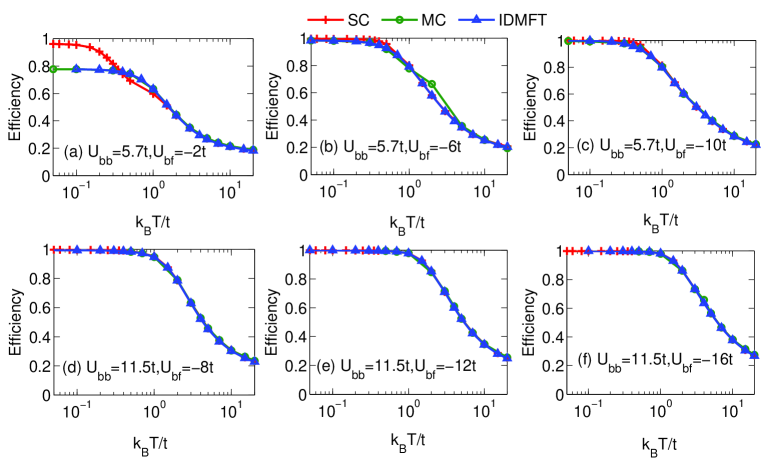
Figure 1: (Color on-line) Efficiency $\mathcal{E}$ as a function of temperature calculated by the SC (red cross), IDMFT (blue triangle) and MC (green circle) methods. The interaction parameters, $U_{bb}$ and $U_{bf}$, are shown in each plot. In (a), the SC calculation differs from the other two methods for $T<1t/k_{B}$. For this region, the SC expansion formulas derived here are no longer accurate. In (b)-(f), all three methods give almost identical results. These calculations also show that almost 100% efficiency is reached for relatively strong attraction, $U_{bf}\geq-6t$, at low temperature, $T<t/k_{B}$.

For a perturbative method like the SC expansion method, it is always necessary to determine the parameter regions where the approximation is valid. Here, we use the previous results obtained from IDMFT and MC methods jim_eff as a reference to determine the accuracy of the SC calculation. It is also worthwhile to notice that the three methods require substantially different computational times. The SC calculation usually takes less than 1 CPU hour while for the same system the IDMFT calculation takes on the order of $10^{5}$ CPU hours. We consider all the parameters used in the previous work jim_eff . The lattice is $50\times 50$ square lattice with the trap frequency $\Omega$ for both species fixed at $\hbar\Omega/2ta=1/11$. The parameters $U_{bf}$ and $U_{bb}$ are chosen based on a typical experimental setup : $U_{bf}/t=-8,\,-12,\,-16$ for $U_{bb}/t=11.5$ and $U_{bf}/t=-2,\,-6,\,-10$ for $U_{bb}=5.7$. The total number of bosons and fermions are set to be 625. We consider the temperature range $0.05t/k_{B}$ to $20t/k_{B}.$

In Fig. 1, we show the efficiency as a function temperature calculated with the three methods. Overall, we find excellent agreement between the SC result and the IDMFT and MC calculations and it is clear that high (unit) efficiency can be achieved when the temperature is low ($T\sim 0.1t/k_{B}$) and the interaction is large compared with $t$. In the case of $U_{bf}=-2t$ and $U_{bb}=5.7t$, the SC calculation starts to deviate greatly from the IDMFT and MC calculation when $T\leq 1t/k_{B}$. It is worth noting that for $T>1t/k_{B}$, the SC calculations agree nicely with the other methods even for a relatively weak cross-species interaction, $U_{bf}=-2t$.

The difference between the SC calculation and the other two methods can be understood from the fact that the SC method is a perturbative method based on the atomic limit of the Hamiltonian, $t=0$ and that the properties derived from the SC expansion are dominated by the atomic-limit behavior with relatively small corrections from the hopping. In the atomic limit, bosons and fermions are completely localized and the only density fluctuations are due to thermal fluctuations. For the low density case considered here, the bosons always form a plateau of unit filling at the center of trap at low temperature and the fermions are attracted by the bosons one by one and form an almost identical plateau. The efficiency therefore always converges to unity as temperature deceases. In Fig. 1, we indeed find the efficiency from the SC calculation always goes to one at low temperatures. The convergence to unity is also true for the IDMFT and MC calculations for all the parameters except for $U_{bf}/t=-2$ and $U_{bb}/t=5.7$. That’s where the SC calculation differs from the IDMFT and MC calculation. It is reasonable to assume that the SC calculation can be applied to the region where the ground state of the system is a localized, Mott insulator like state.

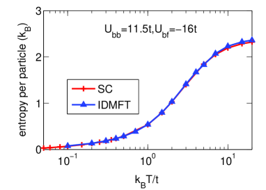
Figure 2: (Color on-line) (a) Entropy per particle as a function of temperature $T$. The SC calculation is marked with red crosses and the IDMFT calculation by the blue line. We find excellent agreement between the SC calculation and the IDMFT calculation.

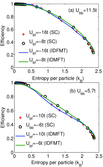
Figure 3: (Color on-line) Efficiency as a function of entropy per particle for different interaction parameters. Note here that we didn’t include the case of $U_{bf}=-2t$, because it is already shown in Fig. 1 that the SC calculation is not accurate for low temperatures in this case. In (a) and (b), we consider two different bosonic interaction strengths and five different inter-species interaction strengths. For all parameters, the efficiency reaches $100\%$ when the entropy is very low. For an intermediate entropy, with an entropy per particle around $1k_{B}$, the efficiency is around $80\%$.

The SC calculation of the entropy per particle is also compared with the IDMFT and MC calculations for all the parameters using Eqs. (44-47). The conclusion of the comparison is similar with the efficiency calculation, that the SC calculation is accurate except for $U_{bf}=-2t$. In Fig. 2 we use one example, $U_{bb}=11.5t$ and $U_{bf}=-16t$, to represent all the cases where the SC calculation agrees with the IDMFT calculation. As the temperature increases, the entropy per particle starts to saturate at around $\sim 2.3k_{B}$. In the next section, we will show that this saturation is actually the result of finite-size effects.

In Fig. 3, we show the behavior of the efficiency as a function of the entropy per particle. This figure can be compared with Fig. 2 in Ref. jim_eff , where the IDMFT calculation is discussed. We verify the findings from the previous work that for strongly attractive inter-species interactions, an efficiency of $100\%$ can be achieved at low temperature (low entropy) region. For an entropy per particle around $1k_{B}$, a $80\%$ efficiency can still be reached. This efficiency is much higher than what has been achieved in experiment Jin_science .

In the following discussion on the SC calculation result, we no longer consider the case of $U_{bf}=-2t$. This is also based on the consideration that the interaction of $U_{bf}=-2t$ is too weak to achieve the desired high efficiency of pre-formed molecules and therefore is not in the parameter region of the main interest in this paper.

IV.2 Finite-size effects

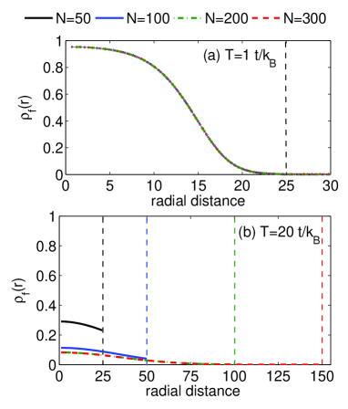
Figure 4: (Color on-line) Finite-size effects on the radial density profile. We assume a two-dimensional $N\times N$ square lattice with hard-wall boundary conditions. The dotted lines indicate the boundaries of different lattices.The interaction parameters are $U_{bf}=-16t$, $U_{bb}=11.5t$. We use the density distribution of the fermionic particle to represent the general dependence of density on the lattice size. In (a), we consider the case of low temperature, $T=t/k_{B}$. Here, the density distribution is concentrated at the center of the trap and there is no difference between different lattice sizes. In (b), we consider the case of high temperature at $T=20t/k_{B}$. Here, the density is confined mainly by the size of the lattice. For $N=50$, the density is confined at the edge of the lattice, $r=25$. For $N=100$, the density is again confined at the edge, $r=50$. For both $N=200$ and $300$, the density goes to zero before reaching the edge of the lattice and the two distributions overlap with each other. We estimate that finite-size effects are eliminated for the $300\times 300$ square lattice for the trap frequency and number of particles considered here.

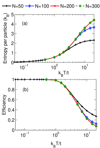
Figure 5: (Color on-line) Finite-size effects on the entropy per particle and the efficiency. We assume a two-dimensional $N\times N$ square lattice with hard-wall boundary conditions. The interaction parameters are $U_{bf}=-16t$, $U_{bb}=11.5t$. In (a), we show the behavior of the entropy per particle as a function of temperature for different system sizes. We see the entropy is significantly affected by the finite size when the lattice is smaller than around $200\times 200$. The finite-size effect is not noticeable at lower temperature ($T<1t/k_{B}$).

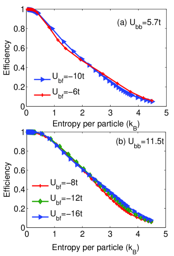
Figure 6: (Color on-line) Efficiency as a function of entropy per particle for a $300\times 300$ square lattice system. We consider 625 atoms for each species. Compared with Fig. 3, the efficiency is significantly higher for the same value of the entropy per particle in the $300\times 300$ lattice system when the entropy per particle is large. On the other hand, the behavior is similar in both lattice systems when the entropy per particle is less than 1$k_{B}$. The unit efficiency is reached roughly when the entropy per particle is less than 0.5$k_{B}.$

In our calculations, we always assume a hard-wall boundary condition at the edge of the lattice. In experiments, however, the atoms are confined only by the trapping potential. This additional confinement imposed by the boundary condition can potentially affect the accuracy of our calculation. This finite-size effect can be neglected if the system is so large that the atoms trapped by the trapping potential almost never reach the edge the system. This, however, is not always the case for the $50\times 50$ lattice. This problem is difficult to address with the IDMFT and MC methods, because of the high computational costs. The SC method, on the other hand, can calculate much larger systems for a fraction of the cost.

In this section, we discuss our calculation for different lattice sizes and discuss finite-size effects for different lattice sizes. To benchmark the SC calculations, the trap frequency and the total number of particles are fixed for all different lattice sizes. We assume the largest lattice sizes are sufficient to neglect the finite-size effects. In Fig. 4, we show the density profile as a function of the lattice size at two temperatures, $T=1t/k_{B}$ (a) and $T=20t/k_{B}$ (b). Here Fig. 4 (a) represents the scaling behavior in the low-temperature region, where there is no significant difference between different lattice sizes and Fig. 4 (b) represents the scaling behavior in the high-temperature region, where the system of small lattice size is highly affected by the boundary effect. Note that the horizontal axes are different scales in the two panels. The parameters used in the plots are $U_{bf}=-16t$ and $U_{bb}=11.5t$. We find similar behavior of the density profile for all the other parameters.

In Fig. 5 (a), we show entropy per particle as a function of temperature at different lattice sizes. In this plot, we find that for small lattices, the entropy per particle becomes saturated at high temperature, while for large lattices it keep increasing as the temperature increases. The saturation is understood as the result of the finite-size effects. When the temperature is high, atoms tend to expand to a larger area in the trap, which leads to a large cloud size and higher entropy. When atoms expand to the edge of the lattice, the possible occupied sites are now constrained and the entropy stays similar even though the temperature increases, hence the saturation. When the lattice is sufficiently large, atoms can freely expand as the temperature increases and the entropy keeps increasing.

The confinement of the atomic cloud in high temperature also affects the efficiency calculation. In Fig. 5 (b), we find that the efficiency saturates to a higher value for smaller lattices. This is because the confinement increases the density overlap between the two species. In the low temperature region, the atoms are close to unit filling at the center of the trap and the efficiency is similar for all difference lattice sizes.

We find that a lattice of $300\times 300$ sites is sufficient to eliminate the finite-size effects for our parameter regions. Hence, we use this lattice size for the efficiency and entropy per particle calculations. In fig. 6, we show the result for the efficiency as a function of the entropy per particle. We estimate the calculation result from the $50\times 50$ lattice is accurate when the temperature is around or below $T=1.25t/k_{B}$.

V Thermometry

V.1 Temperature and Density fluctuations

Based on the fluctuation-dissipation theorem, the compressibility can be related to the density fluctuations as Thermo_Qi ,

$$\kappa=\frac{\partial\rho(r)}{\partial\mu}=\frac{1}{k_{B}T}\left[\langle\rho(r)N\rangle-\langle\rho(r)\rangle\langle N\rangle\right],$$ (48)

where $\rho(r)$ is the radial density profile, $\mu$ is the chemical potential and $N$ is the total number of particles. For a system with a spherically symmetric harmonic trapping potential, $-V_{t}r^{2}$, the local chemical potential at a radial distance $r$ is $\mu-V_{t}r^{2}$. Within the local density approximation, the trapping potential is interpreted as a variance in the chemical potential and the compressibility in the trapped system can be re-written as a function of the density gradient,

$$\frac{\partial\rho(r)}{\partial\mu}=-\frac{1}{2V_{t}r}\frac{\partial\rho(r)}{\partial r}.$$ (49)

These two equations lead to a simple relationship between the density gradient and the density fluctuations in the trapped system,

$$-\frac{1}{2V_{t}r}\frac{\partial\rho(r)}{\partial r}=\frac{1}{k_{B}T}\left[\langle\rho(r)N\rangle-\langle\rho(r)\rangle\langle N\rangle\right].$$ (50)

Based on this relationship, one can determine the temperature from the independently measured density gradient and density fluctuations. For a two dimensional system, a simplified relationship can be found by integrating the above equation over all the two dimensional plane,

$$\frac{\pi}{V_{t}}\rho(0)=\frac{1}{k_{B}T}\left(\langle N^{2}\rangle-\langle N\rangle^{2}\right).$$ (51)

Here, $\rho(0)$ stands for the density at the center of the trap.

With the development of in situ measurements, it is now possible to measure the density gradient and the fluctuations Ketterle_nfluc_thermF ; chin in experiment and this thermometry scheme has shown promise to be a reliable way of estimating the temperature Thermo_Qi ; Thermo_Qi_Troyer . Here we test this method for the Bose-Fermi mixtures and Eqs. (50 and 51) are extended to mixtures by considering the density as the total density of both species and the total number as the total number of both species. With the SC method, we calculate the density gradient directly from the density profile expressions. To simulate the fluctuations measured in the experiments, we use a simplified MC simulation explained in the next section.

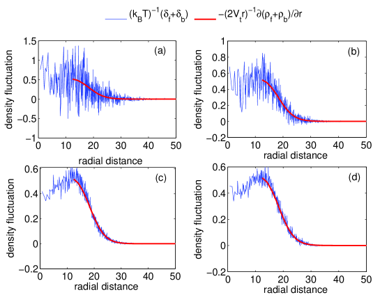
Figure 7: (Color on-line) Density fluctuations averaged over different numbers of samples. The density fluctuations shown here are the total density fluctuations divided by the input temperature, $T=2tk_{B}^{-1}$. All the fluctuations are compared with $-(2V_{t}r)^{-1}\partial(\rho_{b}+\rho_{f})/\partial r$. According to Eq. (50), these two quantities should be equal to each other. In (a)-(c), the total number of configuration generated is $2\times 10^{5}$, with a different sampling strategy. In (a), one sample is taken at every $10^{3}$ configurations, which gives a total of 200 samples to average over. The statistical error in this case is very large. In (b), one sample is taken at every $100$ configurations, which gives a total of 2000 samples. The statistical error is reduced compared with (a). In (c), the total number of samples is $2\times 10^{4}$. The statistical error is the smallest among (a) to (c). In (d), a total of $2\times 10^{6}$ configurations are generated and $2\times 10^{4}$ samples are taken at every 100 configurations.

V.2 Fluctuation calculation

The MC simulation method generates a large collection of states (or configurations) that satisfies the thermal equilibrium criteria. Such collection of states constitutes a thermal ensemble. In the ensemble, each state (or configuration) gives one density distribution, analogous to one single shot image of the density in the experiment. By averaging over all configurations, one obtains the averaged distribution of particles. Deviations between different configurations are the fluctuations. In our simplified MC method, we use the SC method to determine the density distribution for a given temperature and then use the probability as a reference for configuration generation. The ensemble of configurations is decided to be large enough if it can reproduce the input probabilities.

Determining the joint probability : the joint probability, $P_{n,m}^{j}$, is the joint probability of having $n$ bosons and $m$ fermions at site $j$. For $m=1$, the joint probability of having $n$ bosons and $1$ fermion at site $j$ can be found from the fermionic density distribution, similar to the calculation of the local efficiency $\mathcal{E}_{j}$ (indeed, $\mathcal{E}_{j}=P_{1,1}^{j}$),

$$P_{n,1}^{j} = P_{n,1}^{j(0)}-P_{n,1}^{j(1)}+P_{n,1}^{j(2)},$$ (52)

where we again write the probability as a sum of the probability in the atomic limit,

$$P_{n,1}^{j(0)} = \frac{\phi_{b,j}(n)\phi_{f,j}(n)}{\mathcal{Z}_{j}^{(0)}},$$ (53)

and the contributions from the hopping,

$$P_{n,1}^{j(1)} = \beta\sum_{k}\frac{\phi_{b,j}(n)\phi_{f,j}(n)}{\mathcal{Z}_{j}^{(0)}}\times$$ (54)

$$\sum_{n_{b,j},n_{b,k}}\left[\frac{\phi_{b,j}(n_{b,j})\phi_{b,k}(n_{b,k})}{\mathcal{Z}_{j}^{(0)}\mathcal{Z}_{k}^{(0)}}\right.$$

$$\times\left.\frac{\phi_{f,j}(n_{b,j})-\phi_{f,k}(n_{b,k})}{\bar{\mu}_{f,j}(n_{b,j})-\bar{\mu}_{f,k}(n_{b,k})}\right]$$

$$P_{n,1}^{j(2)} = \sum_{k}\sum_{n_{b,k}}\frac{\phi_{b,j}(n)\phi_{b,k}(n_{b,k})}{\mathcal{Z}_{j}^{(0)}\mathcal{Z}_{k}^{(0)}}\times\left[\frac{\beta\phi_{f,j}(n)}{\bar{\mu}_{f,j}(n)-\bar{\mu}_{f,k}(n_{b,k})}\right.$$ (55)

$$+\left.\frac{\phi_{f,k}(n)-\phi_{f,j}(n_{b,k})}{\left[\bar{\mu}_{f,j}(n)-\bar{\mu}_{f,k}(n_{b,k})\right]^{2}}\right].$$

Once the joint probability $P_{n,1}^{j}$ is determined, the complementary probability $P_{n,0}^{j}$ is found based on the relationship in the atomic limit,

$$\sum_{n}\left[P_{n,1}^{j(0)}+\frac{\phi_{b,j}(n)}{\mathcal{Z}_{j}^{(0)}}\right]=1.$$ (56)

Taking into the account the hopping contributions, we can write $P_{n,0}^{j}$ as,

$$P_{n,0}^{j} = \frac{\phi_{b,j}(n)}{\mathcal{Z}_{j}^{(0)}}+P_{n,1}^{j(1)}-P_{n,1}^{j(2)}.$$ (57)

We assume each lattice site is independent and the joint probability at site $j$ is sufficient to determine the density distribution at site $j$. The joint probabilities are evaluated for all the lattice sites and stored in a table before the MC procedure.

Simulation procedure: we use a random number generator to generate configurations with reference to the joint probability table. Specifically the simulation includes the following steps:

1) Create a table for the values of $\widetilde{P}_{n,m}^{j}$ corresponding to the sum of the joint probability of having up to $n$ bosons and up to $m$ fermions at site $j=1$, i.e.

$$\widetilde{P}_{n,m}^{j}=\sum_{k=0}^{n}\sum_{l=0}^{m}P_{k,l}^{j}.$$ (58)

2) Generate a random number $x$ between 0 and 1.

3) Find the smallest $\widetilde{P}_{n^{\prime},m^{\prime}}^{j}$ that is larger than $x$. The number of bosons and fermions at site $j$ is then equal to $n^{\prime}$ and $m^{\prime}$.

4) Repeat steps (2) and (3) to another site, $j=2$, until all the lattice sites are considered. Store the configuration.

5) Repeat steps (2)-(4) $\mathcal{N}$ times to generate $\mathcal{N}$ configurations.

To avoid auto-correlation between adjacent configurations, we choose every other $\mathcal{M}\gg 1$ configurations as samples. The total number of samples is then $N_{s}=\mathcal{N}/\mathcal{M}$. Averaging over all the samples, we obtain the fermionic and bosonic part of the density fluctuation as

$$\delta_{f(b)}(r)=\langle\rho_{f(b)}(r)(N_{f}+N_{b})\rangle-\langle\rho_{f(b)}(r)\rangle\langle N_{f}+N_{b}\rangle,$$ (59)

and the total density fluctuation is the sum of $\delta_{f}$ and $\delta_{b}$. The total number fluctuation is defined as

$$\Delta=\langle\left(N_{f}+N_{b}\right)^{2}\rangle-\langle N_{f}+N_{b}\rangle^{2}.$$ (60)

Here the bracket stands for the averaging over all samples in analogy to the experimental measurement of the fluctuations.

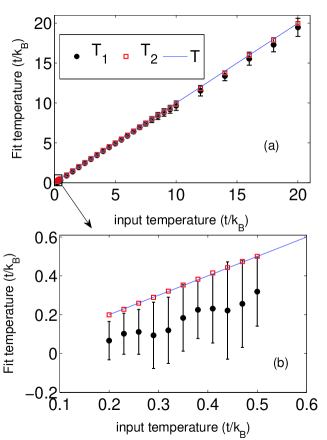
Figure 8: (Color on-line) Extracted temperature as a function of the input temperature. The fluctuations are obtained from $2\times 10^{4}$ samples out of $2\times 10^{6}$ configurations. The value of $T_{1}$ is the mean of $T_{1}(r)$ averaged over $12<r/a<25$ and the error-bar for $T_{1}$ is the standard deviation in $T_{1}(r)$ [Eq. (61)]. The value of $T_{2}$ is obtained through Eq. (62). The input temperature $T$ is drawn as a straight blue line in both plots. In (a), we show our result for the full range of the input temperature, from $T=0.2t/k_{B}$ to $20t/k_{B}$. In this plot, we find very good overall agreement of $T_{1}$ and $T_{2}$ with the input temperature for the temperature range considered, particularly for $T>1t/k_{B}$. In (b), we blow-up the area inside the black square in (a), which corresponds to the low temperature region, where $T=0.2t/k_{B}$ to $0.5t/k_{B}$. In this region, we find that $T_{1}$ shows large relative fluctuations (deviation) from the mean value and the mean value of $T_{1}$ differs relatively greater from $T$. The extracted temperature $T_{2}$ however still shows excellent agreement with the input temperature.

V.3 Results

The fluctuation calculation is carried out for a $300\times 300$ lattice with all five sets of parameters. Overall we find very similar behavior for all the parameters and we use parameters $U_{bb}=11.5t$ and $U_{bf}=-16t$ as an example. In our simulation, the fluctuations between different configurations are from both the random number generator and the thermal fluctuations. The difference between them is that the thermal fluctuations are independent of ensemble sizes and the sampling size. We find that the correct thermal fluctuation calculation requires a large number of samples ($\sim 10^{4}$) and large ensemble sizes ($\sim 10^{6}$). Because of the similarity between the simulation and experimental measurement, this may suggest that a large number of shots are needed in the experiments to obtain the correct thermal fluctuations. Note that we consider here the results from a single plane as one shot, not the averaged results over many planes as reported in Ref. Thermo_Qi_Troyer .

In Fig. 7, we discuss the sampling effects by comparing the fluctuations obtained from different samples with the compressibility calculated from the density gradient $(2V_{t}r)^{-1}\partial\left[\rho_{f}(r)+\rho_{b}(r)\right]/\partial r$. When the number of samples are small, the fluctuations are largely random deviations from the average value. In Fig. 7 (a), the fluctuations can be equally positive and negative, which does not even satisfy the condition that the total fluctuations should be always positive. As the number of samples grows, the random noise starts to be averaged out and the fluctuations start to agree with the fluctuation-dissipation theorem. In Fig. 7 (c), the fluctuations agree very nicely with the relationship predicted by Eq. (50). To show that $10^{4}$ samples are sufficient, we consider an even larger ensemble, with $2\times 10^{6}$ configurations [Fig. 7(d)] and find that the two ensembles produce almost identical results. This shows that the fluctuation calculations obtained in this way are independent of the ensemble size and should correspond to the thermal fluctuations of the system.

With Eqs. (50) and (51), we define two extracted temperatures, $T_{1}$ and $T_{2}$. Let $T_{1}(r)$ be the extracted temperature obtained in terms of the density fluctuations and the density gradient,

$$k_{B}T_{1}^{\prime}(r)=\frac{\delta_{f}(r)+\delta_{b}(r)}{(2V_{t}r)^{-1}\partial(\rho_{f}(r)+\rho_{b}(r))/\partial r},\,12<r/a<25.$$ (61)

Here, we choose the radial distance to be larger than 12 lattice sites because the quantity $(2V_{t}r)^{-1}\partial(\rho_{f}(r)+\rho_{b}(r))/\partial r$ diverges as $r\rightarrow 0$ for a finite density gradient and for small $r$, it goes to zero as the density develops a plateau at unit filling at low temperature. The radial distance is less than 25 lattice sites, because the density is almost zero in the outer regions and that increases the relative error. Together, we find that $r$ between 12 and 25 sites to be the best region to fit the fluctuation and the compressibility with each other. We also note that Eq. (50) still holds if one considers just the fermionic or bosonic part of the system, i.e. keep only the index $f$ or $b$ in $\delta$ and $\rho$.

The temperature $T_{2}$ is obtained based on Eq. (51), which translates into the following expression for the Bose-Fermi mixture,

$$k_{B}T_{2}=\frac{\Delta}{\pi V_{t}^{-1}\left[\rho_{f}(0)+\rho_{b}(0)\right]}.$$ (62)

Here $\rho_{f}(0)$ is the density of fermions at the center of the trap and $\rho_{b}(0)$ the density of bosons at the center of the trap.

In Fig. 8, we show $T_{1}$ and $T_{2}$ as a function of input temperature. Overall, we find very good agreement between $T_{1}$ and $T_{2}$ with the input temperature [Fig. 8 (a)]. We also find in the low temperature region, $T_{2}$ generally fits better with the input temperature [Fig. 8 (b)]. This finding suggests that the statistical error introduced by the numerically generated ensemble is lower in the calculation of $T_{2}$ and this could be because the calculation of $T_{2}$ only involves the first-order observable, the density and the total number fluctuation, whereas, for the calculation of $T_{1}$, we need to calculate the second-order observable, the density fluctuation, which may be more susceptible to statistical errors in the numerical simulation.

VI Conclusion

The SC expansion method is a very efficient way of studying thermal properties of strongly interacting systems. Through comparison with the IDMFT and MC calculations, we show that the strong coupling expansion method can be used for a wide range of parameters even at low temperature when the attractive interaction between the two species is relatively strong. We use the SC method to evaluate the finite-size effects in our previous calculations. This leads to important modifications of the efficiency and the entropy per particle at high temperature. The SC calculation also provides a way to simulate experimental measurements of the fluctuations. Based on the simulation, we find that the thermometry proposal based on the fluctuation-dissipation theorem is accurate for heavy-bose-light-fermi mixtures. This scheme suggests an effective thermometry scheme that works in the extreme low temperature in the deep lattice region. Overall, our work shows a promising way of creating strongly interacting quantum degenerate dipolar matter by loading the mixtures onto an optical lattice before the molecule formation. In addition to higher efficiency, the molecules created in this way are already situated in the optical lattice and can be directly adjusted to realize the novel quantum phases that require the presence of a lattice. It is also worth noting that the SC approach can be used to study other mixtures with modifications. For Fermi-Fermi mixtures like ⁶Li-⁴⁰K, it would require just truncating the heavy bosonic states. For Bose-Bose mixtures like ⁸⁷Rb-¹³³Cs Nagerl , the modification requires allowing for the superfluid order to occur.

- (1) L. D. Carr, D. DeMille, R. V. Krems, and J. Ye, New J. Phys. 11, 055049 (2009).
- (2) S. Ospelkaus, K.-K. Ni, D. Wang, M. H. G. de Miranda, B. Neyenhuis, G. Quéméner, P. S. Julienne, J. L. Bohn, D. S. Jin, J. Ye, Science 327, 853 (2010).
- (3) H. P. Büchler, A. Micheli and P. Zoller, Nature Physics 3, 726 (2007).
- (4) L. Santos, G. V. Shlyapnikov, P. Zoller, and M. Lewenstein, Phys. Rev. Lett. 85, 1791(2000); K. Góral, L. Santos, and M. Lewenstein, Phys. Rev. Lett. 88, 170406 (2002).
- (5) B. Capogrosso-Sansone, C. Trefzger, M. Lewenstein, P. Zoller, and G. Pupillo, Phys. Rev. Lett. 104, 125301 (2010).
- (6) D. DeMille, Phys. Rev. Lett. 88, 067901 (2002).
- (7) C. Ospelkaus, S. Ospelkaus, L. Humbert, P. Ernst, K. Sengstock, and K. Bongs, Phys. Rev. Lett. 97, 120402 (2006).
- (8) J. J. Zirbel, K.-K. Ni, S. Ospelkaus, T. L. Nicholson, M. L. Olsen, P. S. Julienne, C. E. Weiman, J. Ye, and D. S. Jin, Phys. Rev. A 78, 013416 (2008).
- (9) J. M. Sage, S. Sainis, T. Bergeman, and D. DeMille, Phys. Rev. Lett. 94, 203001 (2005).
- (10) C. Weber, G. Barontini, J. Catani, G. Thalhammer, M. Inguscio, and F. Minardi, Phys. Rev. A 78, 061601(R) (2008).
- (11) J. J. Zirbel, K.-K. Ni, S. Ospelkaus, J. P. D’Incao, C. E. Wieman, J. Ye, and D. S. Jin, Phys. Rev. Lett. 100, 143201 (2008).
- (12) G. Thalhammer, K. Winkler, F. Lang, S. Schmid, R. Grimm, and J. H. Denschlag, Phys. Rev. Lett. 96, 050402 (2006); K. Pilch, A. D. Lange, A. Prantner, G. Kerner, F. Ferlaino, H.-C. Nägerl, and R. Grimm, Phys. Rev. A 79, 042718 (2009).
- (13) K. M. Jones, E. Tiesinga, P. D. Lett, and P. S. Julienne, Rev. Mod. Phys. 78, 483 (2006).
- (14) S. Ospelkaus, A. Pe’er, K.-K. Ni, J. J. Zirbel, B. Neyenhuis, S. Kotochigova, P. S. Julienne, J. Ye and D. S. Jin, Nature Physics 4, 622 (2008).
- (15) K.-K. Ni, S. Ospelkaus, M. H. G. de Miranda, A. Pe’er, B. Neyenhuis, J. J. Zirbel, S. Kotochigova, P. S. Julienne, D. S. Jin, J. Ye, Science 322, 231 (2008).
- (16) D. Jaksch, V. Venturi, J. I. Cirac, C. J. Williams, and P. Zoller, Phys. Rev. Lett. 89, 040402 (2002).
- (17) J. K. Freericks, M. M. Maśka, A. Hu, T. M. Hanna, C. J. Williams, P. S. Julienne and R. Lemański, Phys. Rev. A 81, 011605 (2010); ibid. 82, 039901(E) (2010).
- (18) L. Mathey, S.-W. Tsai, and A. H. Castro Neto, Phys. Rev. Lett. 97, 030601 (2006).
- (19) L. M. Falicov and J. C. Kimball, Phys. Rev. Lett. 22, 997 (1969).
- (20) C. Ates and K. Ziegler, Phys. Rev. A 71, 063610 (2005).
- (21) M. Iskin and J. K. Freericks, Phys. Rev. A 80, 053623 (2009).
- (22) C. Gruber and N. Macris, Helv. Phys. Acta 69, 850 (1996); J. Jedrzejewski and R. Lemański, Acta Phys. Pol. B 32, 3243 (2001).
- (23) M. M. Maśka, R. Lemański, J. K. Freericks, and C. J. Williams, Phys. Rev. Lett. 101, 060404 (2008).
- (24) L. Pollet, C. Kollath, K. V. Houcke, and M. Troyer, New J. Phys. 10, 065001 (2008);
- (25) I. Bloch, J. Dalibard, and W. Zwerger, Rev. Mod. Phys. 80, 885 (2008).
- (26) P. B. Blakie and J. V. Porto, Phys. Rev. A 69, 013603 (2004).
- (27) F. Gerbier, Phys. Rev. Lett. 99, 120405 (2007); D. McKay, M. White, and B. DeMarco, Phys. Rev. A 79, 063605 (2009); A. Hoffmann and A. Pelster, Phys. Rev. A 79, 053623 (2009); D. Baillie and P. B. Blakie, Phys. Rev. A 80, 033620 (2009).
- (28) L. Pollet, C. Kollath, K. V. Houcke, and M. Troyer, New J. Phys. 10, 065001 (2008).
- (29) D. McKay, M. White, and B. DeMarco, Phys. Rev. A 79, 063605 (2009).
- (30) B. Capogrosso-Sansone, E. Kozik, N. Prokof’ev, and B. Svistunov, Phys. Rev. A 75, 013619 (2007).
- (31) Q. Zhou, T.-L. Ho, arXiv:0908.3015.
- (32) M. Olshanii and D. Weiss, Phys. Rev. Lett. 89, 090404 (2002).
- (33) F. Gerbier, A. Widera A, S. Fölling, O. Mandel, T. Gericke and I. Bloch, Phys. Rev. Lett. 95 050404(2005);
- (34) M. Popp, J.-J. Garcia-Ripoll, K. G. Vollbrecht, and J. I. Cirac, Phys. Rev. A 74, 013622 (2006); T.-L. Ho and Q. Zhou, Proc. Natl. Acad. Sci. U.S.A. 106, 6916 (2009); J.-S.Bernier, C. Kollath, A. Georges, L. De Leo, F. Gerbier, C. Salomon, and M. Köhl , Phys. Rev. A 79, 061601(R) (2009).
- (35) B. Capogrosso-Sansone, E. Kozik, N. Prokof’ev, and B. Svistunov, Phys. Rev. A 75, 013619 (2007).
- (36) G. Pupillo, C. J. Williams, and N. V. Prokof’ev, Phys. Rev. A 73, 013408 (2006).
- (37) A. Hoffmann and A. Pelster, Phys. Rev. A 79, 053623 (2009).
- (38) C. Sanner, E. J. Su, A. Keshet, R. Gommers, Y. Shin, W. Huang, and W. Ketterle, Phys. Rev. Lett. 105, 040402 (2010).
- (39) D. M. Weld, P. Medley, H. Miyake, D. Hucul, D. E. Pritchard, and W. Ketterle, Phys. Rev. Lett. 103, 245301 (2009).
- (40) P. N. Ma, L. Pollet, M. Troyer, Phys. Rev. A 82, 033627 (2010).
- (41) N. Gemelke, X. Zhang, C. Hung and C. Chin, Nature 460, 995 (2009).
- (42) A. D. Lercher, T. Takekoshi, M. Debatin, B. Schuster, R. Rameshan, F. Ferlaino, R. Grimm and H. C. Nägerl, arXiv:1101.1409.