Seeing jets in heavy-ion collisions

Abstract

In these proceedings, we briefly review how jets can be reconstructed in heavy-ion collisions. The main point we address is the subtraction of the large contamination from the underlying event background. We first present the main ingredients needed to define the jets and perform the background subtraction and then discuss the efficiency of the subtraction for different jet algorithms and background-estimation methods.

1 Introduction

Jets, naively seen as a proxy for the hard partons produced in a final state, have always been powerful tools in collider physics. Recently, interest has grown in using jets in heavy-ion (HI) collisions as a probe of the properties of the dense medium created in these collisions.

The main limitation to reconstruct jets in HI collisions is the fact that they have to be isolated from the large Underlying Event (UE), of ${\cal O}(100-300)$ GeV per unit of $y-\phi$ area. This UE contamination to the jet has to be subtracted if one wants to reconstruct its momentum correctly and obtain an unbiased measurement of the effects of the medium.

In practice, both RHIC and the LHC have already accumulated a large amount of data and have tried various approaches to address that issue (see e.g. [1, 2, 3, 4]).

Here, we describe a jet-based method [5] for full jet reconstruction derived from the original proposal [6] for pileup subtraction in $pp$ collisions. We shall first present the method (see eq. (1) below) and describe its main elements: defining a jet, defining its area and estimating the background density per unit area. We shall then study using Monte-Carlo simulations what kind of performances one might expect in practice.

Most of the effects we shall describe below can be estimated analytically. However, since this often involves rather technical arguments, we will not reproduce them in these proceedings and redirect the interested reader to Ref. [5]. Furthermore, we shall concentrate on the situation at the LHC. Similar results are obtained for RHIC and can be found in [5].

2 Defining background-subtracted jets

Master formula

If the background one wants to subtract from the jets is sufficiently uniform, one can characterise it by two numbers: its average transverse-momentum density per unit area $\rho$ and its fluctuations per unit area $\sigma$. For a given jet, the contamination due to the additional background will thus be $\rho A_{\rm jet}\pm\sigma\sqrt{A_{\rm jet}}$, where $A_{\rm jet}$ is a measurement of the area of that jet. To correct for the background contamination, we can thus define a (4-vector) subtracted jet momentum as

$$p_{j}^{\mu,{\rm sub}}=p_{j}^{\mu}-\rho A_{j}^{\mu}\,.$$ (1)

In order to apply that master formula, three building blocks, described below, are necessary: define jets, define their area and estimate the background density $\rho$.

Before getting to that, let us mention that eq. (1) is incomplete in two major aspects. The first one comes from the fluctuations of the background, leaving an uncertainty of the order of $\sigma\sqrt{A_{\rm jet}}$. The second source is referred to as back reaction [7]: since background particles have a non-vanishing momentum, they can affect the clustering of the “hard” particles; this means, on top of the pure background contamination ($\rho A_{\rm jet}$), the hard contents of the jet can change when considering it together with the background. We will show some examples of these effects in Section 3.

Jet definitions

Defining jets from a list of input objects — e.g. particles or calorimeter towers — has been the topic of many discussions over the last few decades (see e.g. [8]). Here, we shall concentrate on recombination-type algorithms that define the distances

$$d_{ij} = {\rm min}(k_{t,i}^{2p},k_{t,j}^{2p})\left(\Delta\phi_{ij}^{2}+\Delta y_{ij}^{2}\right),$$ (2)

$$d_{iB} = k_{t,i}^{2p}R^{2},$$ (3)

respectively between any pair of particles and for a single particle. The clustering works by successively identifying the smallest distance; if it is a $d_{ij}$ recombine particles $i$ and $j$, otherwise, call $i$ a jet.

The geometric factor in $d_{ij}$ basically ensures that collinear particles will be clustered in the same jet. The $k_{t}$-dependent prefactor varies from one algorithm to another: the $k_{t}$ algorithm [9, 10, 11] has $p=1$ so that soft QCD emissions are clustered early in the sequence; the simple case $p=0$ corresponds to the Cambridge/Aachen (C/A) algorithm [12, 13], useful e.g. for jet substructure studies; the anti-$k_{t}$ algorithm [14], $p=-1$, will cluster jets around hard objects, producing hard jets with rigid, circular, shapes. Note that the anti-$k_{t}$ algorithm is the default choice for most of the LHC experiments. All these algorithms are accessible using the FastJet package [15, 16] and we shall fix $R=0.4$ in what follows.

Recently, a lot of progress has been made that involve making use of the substructure of the jets. To illustrate that, we shall consider, on top of the 3 algorithms introduced above, the C/A algorithm supplemented with a filter (C/A(filt)) [17]. The latter works by reclustering each individual jet with a smaller radius (we shall use $R/2$) and only keep the 2 hardest subjets. Because of the collinear nature of QCD branchings, the filtering procedure is expected to keep most of the QCD part of the jet and reject part of the Underlying-Event contamination.

Jet areas

Practically, the area of a jet is defined [7] as the region in which it captures (infinitely) soft particles (ghosts). Here, we will use the active area of jets determined by adding a dense coverage of ghosts to the event, each carrying a “quantum” of area, clustering them together with the jets, and obtain the area by summing the ghost it contains. This procedures mimics the addition of a background to the event with the exception that ghosts are infinitely soft.

The precise details of how the jet area is defined are largely irrelevant. However, we would like to stress that for the computation of the background density (see below), we advise the use of the explicit_ghost option of FastJet [15] to correctly handle empty regions of the event.

Background estimation

In [6], the following method has been suggested: first cluster the event with the $k_{t}$ or C/A algorithm with a radius $R_{\rho}$ to use, as an estimator for the background density per unit area,

$$\rho=\mathrm{median}\left\{\frac{p_{j,t}}{A_{j,t}}\right\},$$ (4)

where the computation of the median includes all the jets up to a maximal rapidity $y_{\rm max}$. We refer to that choice as the global range below.

To better take into account the non-uniformities of the background, we have realised that there is some interest in using only jets in the vicinity of the jet we want to subtract:

$$\rho_{{\cal R(j)}}=\mathrm{median}\left\{\frac{p_{j^{\prime},t}}{A_{j^{\prime},t}}\right\}_{j^{\prime}\in{\cal R(j)}},$$ (5)

where the subscript ${\cal R(j)}$ explicitly refers to the fact that we use a local range centred on the jet $j$ for which we want to estimate the background.

We have considered 3 different options: a CircularRange($\Delta$) keeping jets within a distance $\Delta$ (we used $\Delta=3R$) of the jet, a DoughnutRange($\delta,\Delta$) keeping jets with a distance from the jet between $\delta$ and $\Delta$ (we used $\delta=R$, and $\Delta=2R$ or $3R$) and a StripRange($\Delta$) being a rapidity strip extending between $y_{\rm jet}-\Delta$ and $y_{\rm jet}+\Delta$ (we used $\Delta=2R$ or $3R$).

The use of a median in (4) and (5) rather than an average is made to reduce the effect of the hard jets on the estimation of $\rho$. In order to further reduce that bias, we have also tested the exclusion of the two hardest jets in the event from the jets used for the median computation.

3 Expected performances

Framework

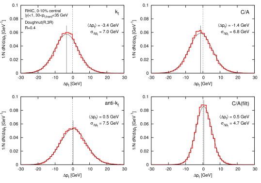
Figure 1: Distribution of $\Delta p_{t}$ (red histograms) at RHIC for each of our 4 jet algorithms, together with a Gaussian (black curve) whose mean (solid vertical line) and dispersion are equal to $\left\langle\Delta p_{t}\right\rangle$ and $\sigma_{\Delta p_{t}}$ respectively.

In this Section, we study how the method presented above performs in practice.

To achieve that, we shall embed $pp$ hard events in HI background, apply our background-subtraction method and see how precisely the original hard jets are reconstructed. The $pp$ events will be generated using Pythia 6.4 [18] and for the $AA$ events we have used Hydjet 1.6 [19]. We note that, for 0-10% central collisions, the HI background has an average density $\langle\rho\rangle$ of about 100 GeV at RHIC and 310 GeV at the LHC, with fluctuations $\langle\sigma\rangle$ around 8 and 20 GeV, respectively.

Jets are reconstructed and subtracted for both the hard event alone and the hard event embedded in the heavy-ion background (which we shall refer to as the full event). We have concentrated on the two hardest jets in the hard event. For each of them, we search for a matching full jet in the full event by requiring that the hard contents of the full jet accounts for at least 50% of the original hard jet.

For a matching pair of jets, we consider the difference between the subtracted full jet and the subtracted hard jet:

$$\Delta p_{t}=p_{t}^{AA,sub}-p_{t}^{pp,sub}.$$ (6)

An efficient background subtraction would directly translate into small $\Delta p_{t}$. Though we could obtain the full distribution of $\Delta p_{t}$, see Fig. 1 for RHIC kinematics, they can be considered as sufficiently Gaussian for the purpose of comparing different background-estimation ranges and jet-reconstruction algorithms, and we shall concentrate on its average $\left\langle\Delta p_{t}\right\rangle$ and dispersion

$$\sigma_{\Delta p_{t}}=\sqrt{\left\langle\Delta p_{t}^{2}\right\rangle-\left\langle\Delta p_{t}\right\rangle^{2}}.$$

An effective subtraction would then be characterised by small values of $\left\langle\Delta p_{t}\right\rangle$ and $\sigma_{\Delta p_{t}}$.

For the results presented below, the $k_{t}$ algorithm with a radius $R_{\rho}=0.5$ has been used for the median-based estimation of the background density.

Choice of range

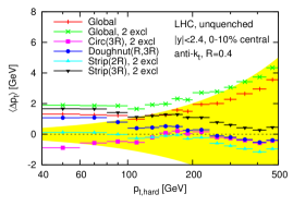
Figure 2: Effect of the choice of range on the average $p_{t}$ shift, $\Delta p_{t}$, as defined in eq. (6), for LHC kinematics. In this figure and those that follow, the yellow band corresponds to 1% of the $p_{t}$ of the hard jet. The label “2 excl” means that the two hardest jets of the event have been excluded from the median computation.

We start our investigation by looking at how the choice of the range made to estimate the background density affect the subtraction. On Fig. 2, we see that for all the ranges we consider, the average uncertainty on the reconstructed jet transverse momentum is $\lesssim$ 1%, with a small preference for local ranges at large $p_{t}$.

In choosing the range, there is a tension between remaining in the vicinity of the jet one wants to subtract and having enough jets in the range to estimate the median properly. As a rule of thumb, it can be shown that a local range needs to contain at least 9 jets to give a reasonable estimate of $\rho$.

For what follows, we shall use the DoughnutRange($R,3R$) as a default choice.

Choice of algorithm

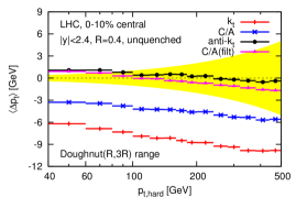
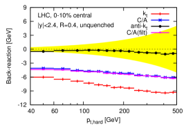
Figure 3: Left: average shift $\left\langle\Delta p_{t}\right\rangle$, as a function of $p_{t,\rm hard}$, shown for the LHC. Right: contribution to $\left\langle\Delta p_{t}\right\rangle$ due to back-reaction. Note that the back-reaction results are independent of the range used for estimating $\rho$ in the heavy-ion event.

We now focus on the dependence on the specific choice of algorithm and first consider the average shift $\left\langle\Delta p_{t}\right\rangle$. It is plotted on Fig. 3(left) for the four algorithms under consideration. We see that while the anti-$k_{t}$ and C/A(filt) algorithms give an average shift close to zero, the $k_{t}$ and C/A algorithms have a larger, negative, shift.

Since the estimation of the background density $\rho$ is common to all 4 algorithms, this can actually be traced back to a difference in back-reaction as seen on Fig. 3 (right). For all except C/A(filt), the differences observed in the average shift correspond to differences in back-reaction and the fact that the anti-$k_{t}$ has a small shift is a direct consequence of its rigidity. In the case of the C/A(filt) the final small shift can be explained by a (fortuitous) cancellation between the offset due to back-reaction and a filtering bias.

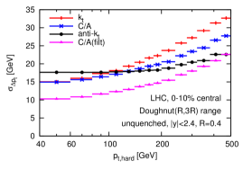
Figure 4: Dispersion $\sigma_{\Delta p_{t}}$ for the LHC kinematics.

Finally, we turn to the dispersion $\sigma_{\Delta p_{t}}$. The observed dispersions for the LHC are shown on Fig. 4. While anti-$k_{t}$ was the more robust in terms of average shift, when we consider the dispersion, C/A(filt) shows better performances. What we really see here is precisely the effect of filtering which practically reduces the area of the jet, thus reducing the dispersion which is proportional to $\sqrt{A_{\rm jet}}$. With our choice of parameters, the area after filtering is about $1/2$ of the original C/A-jet area and we may thus expect a decrease of a factor $1/\sqrt{2}$ in the dispersion, which is consistent with what is observed on the figure at low $p_{t}$.

Additional remarks

To conclude this Section, we want to make a few remarks on other tests that can be performed (see [5] for more details).

First, to test the robustness of our results, we have checked the effect of quenching on the embedded hard events. This can been done e.g. by running PyQuen [20] on the Pythia jets. We have noticed a negligible effect on the results obtained with the anti-$k_{t}$ algorithm and an effect smaller than 2% for the C/A(filt) case.

Then, we can investigate if our conclusions hold for more peripheral collisions, where flow effects may increase the fluctuations. For the average quantities presented here, we have checked that our conclusions remain unchanged in the case of non-central collisions. However, it is interesting to mention that if we study the average shift $\left\langle\Delta p_{t}\right\rangle$ as a function of the azimuthal angle between the jet and the reaction plane, we see oscillations of a few GeV. The use of a range with a finite azimuthal coverage, like the DoughnutRange, reduces these oscillations compared to a StripRange, but further developments would be needed to reduce them completely.

4 Conclusions

To conclude, we have studied the possibility to use the jet-area-based subtraction method initially proposed in [6] to reconstruct full jets in heavy-ion collisions.

We have found that the use of local ranges to reduce the non-uniformities of the background (like its rapidity dependence) improves the background subtraction. It would be interesting to see if using different ranges (bearing in mind that they should contain at least $\sim$9 jets to give a reliable estimate of $\rho$) could help obtaining an unceratinty on the estimation of $\rho$.

We have studied subtraction performances by embedding Pythia events in Hydjet heavy-ion events and measured for the two hardest jets in each event $\Delta p_{t}$, the transverse momentum difference between the original (subtracted) hard jet and the embedded/full jet after subtraction. While knowledge of the full $\Delta p_{t}$ distribution is relevant, e.g. for unfolding purposes [21], we have chosen to focus only on its average and dispersion.

For the average shift $\left\langle\Delta p_{t}\right\rangle$, we have observed that the anti-$k_{t}$ (because of its rigidity) and the C/A algorithm supplemented with a filter give a result close to zero, though one has to notice that for the latter, this is the result of a cancellation between two effects.

In terms of dispersion the C/A(filt) algorithm, which has a smaller sensitivity to the UE, as a consequence of its reduced area, shows better performances than the other algorithms.

Finally, we have noticed (see [5] for more details) that these results also hold when quenched jets are embedded or when one considers more peripheral collisions. In this last case, there is a residual shift when one considers the shift as a function of the azimuthal angle between the jet and the reaction plane that is left for further studies. We also note that, though the C/A filt algorithm has a smaller dispersion, it may be more affected by quenching than the anti-$k_{t}$ algorithm (e.g. because of jet broadening) and it may thus be helpful to consider both to obtain the most complete and valuable information.

Acknowledgements

I am grateful to the organisers of the Hard Probes conference for the opportunity to discuss the results presented here. I also want to thank M. Cacciari, J. Rojo and G. Salam which have contributed to the physics results presented in these proceedings.

References

- [1] S. Salur, Full Jet Reconstruction in Heavy Ion Collisions, Nucl. Phys. A830 (2009) 139c–146c. arXiv:0907.4536, doi:10.1016/j.nuclphysa.2009.09.016.
- [2] M. Ploskon, Inclusive cross section and correlations of fully reconstructed jets in 200 GEV Au+Au and p+p collisions, Nucl. Phys. A830 (2009) 255c–258c. arXiv:0908.1799, doi:10.1016/j.nuclphysa.2009.10.095.
- [3] Y.-S. Lai, Direct jet reconstruction in p + p and Cu + Cu at PHENIXarXiv:0911.3399.
- [4] T. A. Collaboration, Observation of a Centrality-Dependent Dijet Asymmetry in Lead-Lead Collisions at sqrt(S(NN))= 2.76 TeV with the ATLAS Detector at the LHCarXiv:1011.6182.
- [5] M. Cacciari, J. Rojo, G. P. Salam, G. Soyez, Jet Reconstruction in Heavy Ion CollisionsarXiv:1010.1759.
- [6] M. Cacciari, G. P. Salam, Pileup subtraction using jet areas, Phys. Lett. B659 (2008) 119–126. arXiv:0707.1378, doi:10.1016/j.physletb.2007.09.077.
- [7] M. Cacciari, G. P. Salam, G. Soyez, The Catchment Area of Jets, JHEP 04 (2008) 005. arXiv:0802.1188, doi:10.1088/1126-6708/2008/04/005.
- [8] G. P. Salam, Towards Jetography, Eur. Phys. J. C67 (2010) 637–686. arXiv:0906.1833, doi:10.1140/epjc/s10052-010-1314-6.
- [9] S. Catani, Y. L. Dokshitzer, M. H. Seymour, B. R. Webber, Longitudinally invariant clustering algorithms for hadron hadron collisions, Nucl. Phys. B406 (1993) 187–224.
- [10] S. Catani, Y. L. Dokshitzer, M. Olsson, G. Turnock, B. R. Webber, New clustering algorithm for multi - jet cross-sections in annihilation, Phys. Lett. B269 (1991) 432–438.
- [11] S. D. Ellis, D. E. Soper, Successive combination jet algorithm for hadron collisions, Phys. Rev. D48 (1993) 3160–3166. arXiv:hep-ph/9305266.
- [12] Y. L. Dokshitzer, G. D. Leder, S. Moretti, B. R. Webber, Better jet clustering algorithms, JHEP 08 (1997) 001. arXiv:hep-ph/9707323.
- [13] M. Wobisch, T. Wengler, Hadronization corrections to jet cross sections in deep- inelastic scatteringarXiv:hep-ph/9907280.
- [14] M. Cacciari, G. P. Salam, G. Soyez, The anti- jet clustering algorithm, JHEP 04 (2008) 063. arXiv:0802.1189, doi:10.1088/1126-6708/2008/04/063.
- [15] M. Cacciari, G. P. Salam, Dispelling the myth for the jet-finder, Phys. Lett. B641 (2006) 57–61. arXiv:hep-ph/0512210.
- [16] M. Cacciari, G. P. Salam, G. Soyez, http://www.fastjet.fr/.
- [17] J. M. Butterworth, A. R. Davison, M. Rubin, G. P. Salam, Jet substructure as a new Higgs search channel at the LHC, Phys. Rev. Lett. 100 (2008) 242001. arXiv:0802.2470, doi:10.1103/PhysRevLett.100.242001.
- [18] T. Sjostrand, S. Mrenna, P. Z. Skands, PYTHIA 6.4 Physics and Manual, JHEP 05 (2006) 026. arXiv:hep-ph/0603175, doi:10.1088/1126-6708/2006/05/026.
- [19] I. P. Lokhtin, et al., Heavy ion event generator HYDJET++ (HYDrodynamics plus JETs), Comput. Phys. Commun. 180 (2009) 779–799. arXiv:0809.2708, doi:10.1016/j.cpc.2008.11.015.
- [20] I. P. Lokhtin, A. M. Snigirev, A model of jet quenching in ultrarelativistic heavy ion collisions and high-p(T) hadron spectra at RHIC, Eur. Phys. J. C45 (2006) 211–217. arXiv:hep-ph/0506189, doi:10.1140/epjc/s2005-02426-3.
- [21] P. Jacobs, These proceedings.