Analysis of a growing dynamic length scale in a glass-forming binary hard-sphere mixture

Abstract

We examine a length scale that characterizes the spatial extent of heterogeneous dynamics in a glass-forming binary hard-sphere mixture up to the mode-coupling volume fraction $\phi_{c}$. First, we characterize the system’s dynamics. Then, we utilize a new method [Phys. Rev. Lett. 105, 217801 (2010)] to extract and analyze the ensemble independent dynamic susceptibility $\chi_{4}(t)$ and the dynamic correlation length $\xi(t)$ for a range of times between the $\beta$ and $\alpha$ relaxation times. We find that in this time range the dynamic correlation length follows a volume fraction independent curve $\xi(t)\sim\ln(t)$. For longer times, $\xi(t)$ departs from this curve and remains constant up to the largest time at which we can determine the length accurately. In addition to the previously established correlation $\tau_{\alpha}\sim\exp[\xi(\tau_{\alpha})]$ between the $\alpha$ relaxation time, $\tau_{\alpha}$, and the dynamic correlation length at this time, $\xi(\tau_{\alpha})$, we also find a similar correlation for the diffusion coefficient $D\sim\exp[\xi(\tau_{\alpha})^{\theta}]$ with $\theta\approx 0.6$. We discuss the relevance of these findings for different theories of the glass transition.

I Introduction

It is becoming increasingly apparent that growing length scales can be associated with the dramatic slowing down of the dynamics in glass-forming systems. One such length scale characterizes the spatial extent of the so-called dynamic heterogeneity. It has been found that upon approaching the glass transition the particles’ motion becomes increasingly heterogeneous and the particles can be divided into ”slow” and ”fast” sub-sets Sillescu (1999); Ediger (2000); Glotzer et al. (2000); Richert (2002); Andersen (2005). These sub-sets can be seen as distinct peaks in the probability of the logarithm of single particle displacements $P[\log_{10}(\delta r);t]$ Flenner and Szamel (2005a); Reichman et al. (2005); Saltzman and Schweizer (2008). Importantly, the slow and fast particles are not uniformly distributed in space, but form clusters whose size increases as the dynamics slows. The average spatial extent of the clusters of slow particles can be defined as a dynamic correlation length. This dynamic correlation length and other closely related lengths have been studied in simulations Donati et al. (1999); Lacevic et al. (2003); Whitelam et al. (2004); Berthier (2004); Stein and Andersen (2008); Flenner and Szamel (2009); Karamakar et al. (2009); Karamakar et al. (2010a), experiments Berthier et al. (2005a); Dalle-Ferrier et al. (2007); Crauste-Thibierge et al. (2010), and discussed theoretically Biroli and Bouchaud (2004); Biroli et al. (2006); Berthier et al. (2007a, b); Szamel (2008); Szamel and Flenner (2010).

One convenient way to characterize the spatial extent of the clusters is to identify the slow particles and then determine their spatial correlations. In simulational investigations this is typically done by analyzing the so-called four-point dynamic structure factors $S_{4}(q;t)$. The four-point structure factor quantifies spatial correlations between the slow particles. The label “four-point” refers to the fact that $S_{4}(q;t)$ is a correlation function of two two-point functions that are used to characterize particles’ dynamics and to define slow particles. Examples of these two point functions are the microscopic intermediate scattering functions and overlap functions, but other functions have also been used in the literature. Of particular interest are two quantities that can be expressed in terms of $S_{4}(q;t)$: the dynamic susceptibility, $\chi_{4}(t)=\lim_{q\rightarrow 0}S_{4}(q;t)$, which is a measure of the overall strength of the dynamic heterogeneity, and the dynamic correlation length, $\xi(t)$, which characterizes its spatial extent. The relationship between $\chi_{4}(t)$ and $\xi(t)$ provides insight into the fractal dimension of the slow particles clusters.

In spite of a relatively straightforward definition of $\chi_{4}(t)$, its direct simulational evaluation suffers from a technical difficulty. The difficulty originates from the fact that in a typical simulational ensemble some global fluctuations are suppressed. For example, in most simulations of glass-forming liquids the number of particles and the volume is kept constant, thus the density of the system is constant and global density fluctuations do not contribute to the direct simulational calculation of $\chi_{4}(t)$. Berthier et al. Berthier et al. (2005a) proposed that these suppressed fluctuations can be calculated utilizing a procedure derived by Lebowitz et al. Lebowitz et al. (1967). This procedure results in a two-part expression for the dynamic susceptibility, $\chi_{4}(t)=\chi_{4}(t)|_{\mathbf{x}}+\mathcal{X}(t)$ where $\chi_{4}(t)|_{\mathbf{x}}$ is the susceptibility in an ensemble with $\mathbf{x}$ kept fixed (which can readily be obtained from simulations) and $\mathcal{X}(t)$ is a correction term.

Berthier et al. Berthier et al. (2005a) furthermore noted that while $\chi_{4}(t)|_{\mathbf{x}}$ cannot be easily determined experimentally, the correction term $\mathcal{X}(t)$ can. This fact, together with the positive definite character of the former term, $\chi_{4}(t)|_{\mathbf{x}}>0$, provides an experimental lower bound for $\chi_{4}(t)$. However, the relative size of $\chi_{4}(t)$ and the correction term remained an open question. In addition, even if the experimental lower bound was a good estimate of $\chi_{4}(t)$, there was no reliable correlation between $\chi_{4}(t)$ and the dynamic correlation length $\xi(t)$.

The relative size of the two terms contributing to $\chi_{4}(t)$ was investigated by Berthier et al. Berthier et al. (2007a, b) and by Brambilla et al. Brambilla et al. (2009). The main conclusion was that as the dynamics slows, the correction term becomes an increasingly better approximation for the ensemble independent $\chi_{4}(t)$. The assessment and extension of this result is one of the subjects of the present paper.

There were several earlier simulational investigations Lacevic et al. (2003); Whitelam et al. (2004); Berthier (2004); Stein and Andersen (2008); Flenner and Szamel (2009); Karamakar et al. (2009) of the correlation between the dynamic susceptibility $\chi_{4}(t)$ and the correlation length $\xi(t)$ and between the average dynamics (as characterized by, e.g. the $\alpha$ relaxation time, $\tau_{\alpha}$) and $\xi(t)$, but their results, by and large, disagreed Karamakar et al. (2010b). Recently, it has been realized that in order to get reliable results for $\chi_{4}(t)$ and $\xi(t)$ one has to simulate systems considerably larger than was customary Karamakar et al. (2010a, b). In an earlier short note Flenner and G. (2010), we described an application of the method of Lebowitz et al. Lebowitz et al. (1967) to facilitate the determination of $\xi(\tau_{\alpha})$ using large scale, $80\,000$ particles, simulations. We found that $\xi(\tau_{\alpha})\sim\ln(\tau_{\alpha})$ over the full range of densities studied. This slower, logarithmic growth of $\xi(\tau_{\alpha})$ with $\tau_{\alpha}$ is more consistent with experimental findings than the power law growth found in many previous simulations.

In the present paper we give details omitted in Ref. Flenner and G. (2010) due to length restrictions. In addition, we analyze the time dependence of both the dynamic susceptibility and correlation length, and investigate additional correlations between the length and the average dynamics.

We describe the system and simulation method in Sec. II and we briefly characterize the system’s dynamics in Sec. III. Since there is no accepted theory of the glass transition, examination of the system’s dynamics can get bogged down with an extensive number of different fits and fit parameters. Throughout much of the paper we refer to two regimes: a mode-coupling like regime where power laws describe the data well, and a different dynamic regime where the mode-coupling like power laws are not applicable. We discuss this characterization of the data and describe the relevant fits in Appendix A. After describing the system’s dynamics, in Sec. IV we investigate the dynamic susceptibility $\chi_{4}(t)$ and the dynamic correlation length $\xi(t)$. The technical details of the calculation of $\chi_{4}(t)$ and $\xi(t)$ are given in Appendix B. In Sec. V we explore the connections between the dynamic correlation length and the average dynamics. We finish with a discussion in Sec. VI.

II Simulation Details

We simulated a system introduced by Brambilla et al. Brambilla et al. (2009): a 50:50 binary hard-sphere mixture where the diameter $d_{2}$ of the larger sphere is $1.4$ times larger than the diameter $d_{1}$ of the smaller sphere. The size difference is chosen to inhibit crystallization. We studied systems with $N=(N_{1}+N_{2})=80\,000$ particles at volume fractions $\phi=\pi(N_{1}d_{1}^{3}+N_{2}d_{2}^{3})/6V$ equal to 0.4, 0.45, 0.5, 0.52, 0.55, 0.56, 0.57, 0.58, and 0.59 and systems with $10\,000$ particles at volume fractions $\phi$ equal to 0.54, 0.575, 0.58, 0.585, and 0.59. Additional simulations were performed at slightly different volume fractions and concentrations to obtain the derivatives needed in this work. To determine the derivatives with respect to $\phi$, we performed simulations at $\phi\pm\delta\phi$ where $\delta\phi=0.001$ for $\phi\leq 0.58$ and $\delta\phi=0.0005$ for $\phi\geq 0.585$. To determine the derivatives with respect to concentration $c=N_{1}/N$, we performed simulations at $c=0.5\pm 0.05$ for $\phi\leq 0.58$. The concentration derivatives had very little $\phi$ dependence over the range we examined. We found that they were not necessary to obtain accurate correlation lengths and susceptibilities for $\phi\geq 0.56$. Thus we did not determine the concentration derivatives for $\phi\geq 0.585$.

We performed Monte Carlo simulations with the local trial displacements of particles randomly chosen from a cube of length $0.1d_{1}$. It has been shown that Monte Carlo dynamics reproduces well the long time dynamics of glass forming systems Berthier and Kob (2007). Moreover, Brambilla et al. Brambilla et al. (2009) have shown that the present system with this particular Monte Carlo dynamics reproduces well the long-time dynamics of their experimental system - a dense poly-disperse hard sphere system in which hydrodynamic interactions can be neglected.

The simulations were run for at least $100\tau_{\alpha}$ ($\tau_{\alpha}$ is defined in Section III) after the systems stopped aging. To check for the presence of aging, we examined two point and four point quantities to see if they significantly depended on the initial time of the calculation. We found that the dynamic susceptibility $\chi_{4}(t)|_{\phi,c}$ is very sensitive to aging, thus providing a good test of equilibration. We ran at least four production runs at each volume fraction, and the results are an average over those runs. Results are presented in reduced units where the unit of length is $d_{1}$ and the unit of time $t$ is one Monte Carlo step (a Monte Carlo step is one attempted move per particle). Since the center of mass of the system can drift, all positions are calculated with respect to the center of mass (for the calculation of the center of mass position masses of all the particle were taken as identical).

III Single Particle Dynamics

In this section we examine the slowing down of the average dynamics. In addition, we show that there is an indication of dynamic heterogeneity in two-point functions, and the dynamic heterogeneity is increasing with volume fraction.

We start by examining the volume fraction dependence of the $\alpha$ relaxation time, $\tau_{\alpha}$, determined by a characteristic decay time of an average overlap function. The average overlap function is defined as

$$F_{o}(t)=\frac{1}{N}\left<\sum_{n=1}^{N}w_{n}(t)\right>,$$ (1)

where $w_{n}(t)$ is a microscopic overlap function,

$$w_{n}(t)=\Theta[a-|\mathbf{r}_{n}(t)-\mathbf{r}_{n}(0)|].$$ (2)

Here $\Theta(x)$ is Heaviside’s step function and $\mathbf{r}_{n}(t)$ is the position of particle $n$ at a time $t$. The microscopic overlap function $w_{n}(t)$ select particles that did not move farther than $a$ from their original positions during the time $t$. In this work we use $a=0.3$. Correspondingly, the average overlap function $F_{o}(t)$ measures the average fraction of particles which did not move farther than $a$ from their original positions during the time $t$. We will refer to particles which did not move farther than $a$ during time $t$ as the slow particles. Thus,

$$N_{s}(t)=\sum_{n=1}^{N}w_{n}(t)$$ (3)

is the number of slow particles during time $t$, and $\left<N_{s}(t)\right>=NF_{o}(t)$ is the average number of slow particles during time $t$.

$F_{o}(t)$ encodes similar information as the self intermediate scattering function $F_{s}(q;t)=N^{-1}\left<\sum_{n}e^{-\mathbf{q}\cdot[\mathbf{r}_{n}(t)-\mathbf{r}_{n}(0)]}\right>$. Thus, it displays similar characteristics. At high densities a pleateau region develops in the time dependence of $F_{o}(t)$. Moreover, an early $\beta$ relaxation regime can be identified as the decay to the plateau, and then the late $\beta$ regime can be seen as a decay from the plateau. The characteristic time of the final decay from the plateau is referred to as the $\alpha$ relaxation time $\tau_{\alpha}$. We define $\tau_{\alpha}$ adopting the formula used before for the self-intermediate scattering function, $F_{o}(\tau_{\alpha})=e^{-1}$. Consequently, according to this definition the average fraction of slow particles during time $\tau_{\alpha}$ is about 37%.

Shown in Fig. 1(a) is $F_{o}(t)$ for $\phi=0.4$, 0.45, 0.5, 0.52, 0.54, 0.55, 0.56, 0.57, 0.575, 0.58, 0.585, and 0.59 listed from left to right. For small volume fractions the decay is nearly exponential. At higher volume fractions the long time decay follows a stretched exponential form $\exp[-(t/\tau)^{\beta}]$ with a weakly $\phi$ dependent $\beta\approx 0.55$. The stretched exponential relaxation is usually interpreted as an indication of dynamic heterogeneity.

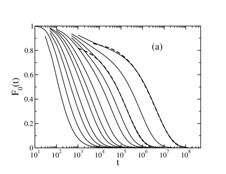
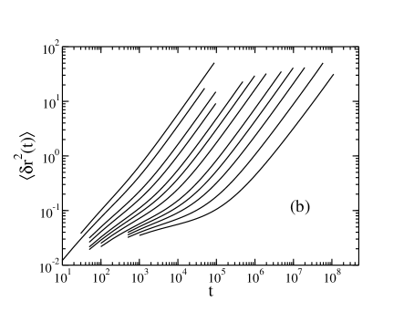
Figure 1: (a): The average overlap function $F_{o}(t)$ for $\phi=0.4$, 0.45, 0.5, 0.52, 0.54, 0.55, 0.56, 0.57, 0.575, 0.58, 0.585, and 0.59 listed from left to right. The dashed lines are stretched exponential, $\exp[-(t/\tau)^{\beta}]$, fits at $\phi=0.58$ ($\beta=0.56$) and $\phi=0.59$ ($\beta=0.54$). (b): The mean square displacement $\left<\delta r^{2}(t)\right>$ for $\phi=0.4$, 0.45, 0.5, 0.52, 0.54, 0.55, 0.56, 0.57, 0.575, 0.58, 0.585, and 0.59 listed from left to right.

The other common way to examine the average dynamics is to investigate the mean square displacement displacement

$$\left<\delta r^{2}(t)\right>=N^{-1}\left<\sum_{n}[\mathbf{r}_{n}(t)-\mathbf{r}_{n}(0)]^{2}\right>,$$ (4)

which is shown in Fig. 1(b). Again, for large $\phi$ a plateau forms at intermediate times, then at long times $\left<\delta r^{2}(t)\right>=6Dt$ where $D$ is the self diffusion coefficient. Both the previously mentioned plateau in the average overlap function $F_{o}(t)$ and the plateau in the mean square displacement $\left<\delta r^{2}(t)\right>$ are associated with the so-called cage effect where particles are temporarily trapped by cages of neighboring particles. We use the long time limiting behavior of $\left<\delta r^{2}(t)\right>$ to obtain the self diffusion coefficient $D$. We define the $\beta$ relaxation time $\tau_{\beta}$ as the inflection point of $\ln[\left<\delta r^{2}(t)\right>]$ versus $\ln(t)$ (we found that it is easier to determine $\tau_{\beta}$ from the $\ln[\left<\delta r^{2}(t)\right>]$ inflection point rather than from the $F_{o}(t)$ inflection point). This inflection point could only be determined for $\phi\geq 0.5$.

Shown in Fig. 2 is the volume fraction dependence of the relaxation time, $\tau_{\alpha}$, and the inverse of the self-diffusion coefficient, $1/D$. As in many glass forming systems, there is an range of volume fractions in which power laws provide good fits to the simulation data. Since the mode-coupling theory predicts power law divergences of both $\tau_{\alpha}$ and $1/D$ Götze (1991), the volume fraction where the power law fits diverge is referred to as the mode-coupling volume fraction $\phi_{c}$. However, there is no true divergence at $\phi_{c}$, the mode-coupling transition is said to be avoided, and there is emergence of new behavior beyond $\phi_{c}$. To quantitatively identify a mode-coupling like region of the dynamics we fit $\tau_{\alpha}$ and $1/D$ to power laws $a(\phi_{c}-\phi)^{-\gamma_{\{\tau,D\}}}$ where $\gamma_{\tau}$ and $\gamma_{D}$ denote the power law exponents for $\tau_{\alpha}$ and $1/D$, respectively (see Appendix A for a detailed description of the fits). We found that power laws describe our data well for $0.55\leq\phi\leq 0.58$ with $\phi_{c}=0.59$. These fits are shown as dashed lines in Fig. 2. We also find that our results for the relaxation time are consistent with a fit suggested by Berthier and Witten Berthier and Witten (2009) and later used by Brambilla et al. Brambilla et al. (2009), $\tau_{\alpha}=\tau_{\infty}\exp[B/(\phi_{0}-\phi)^{2}]$. This fit is shown as the solid line in Fig. 2 (again, see Appendix A for a detailed description of this fit)

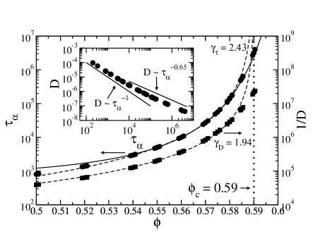
Figure 2: The relaxation time $\tau_{\alpha}$ and the inverse diffusion coefficient $1/D$. The dashed lines are power law fits $a(\phi_{c}-\phi)^{-\gamma}$ and the solid line is a fit suggested by Berthier and Witten Berthier and Witten (2009), $\tau_{\infty}\exp[B/(\phi_{0}-\phi)^{2}]$. Inset: Stokes-Einstein violation: for small volume fractions $D\sim\tau_{\alpha}^{-1}$, whereas for higher volume fraction $D\sim\tau_{\alpha}^{-0.65}$.

In the inset in Fig. 2 we investigate the relation between two quantities discussed above, the $\alpha$ relaxation time and the self-diffusion coefficient. For small $\phi$ we find that $D\sim\tau_{\alpha}^{-1}$ and thus the Stokes-Einstein relation is obeyed. With increasing $\phi$ there appears to be a crossover to a weaker dependence of the self-diffusion coefficient on the $\alpha$ relaxation time. Thus, the Stokes-Einstein relation is violated. The breakdown of this relations is considered to be one of the hallmarks of dynamic heterogeneity.

Quantitatively, we find that for large volume fractions $D\sim\tau_{\alpha}^{-\sigma}$ where $\sigma\approx 0.65$. We should note that for even larger $\phi$ it may be found that $\sigma<0.65$, and our result should be considered an upper bound. A value of $\sigma=0.77$ was found in an experimental glass-former Swallen et al. (2003), and kinetically-constrained lattice-gas models predict a fragility dependent $\sigma$ with values between 0.58 and 0.88 Pan et al. (2005). The Random-First-Order theory also predicts a fragility dependent $\sigma$ Xia and Wolynes (2001).

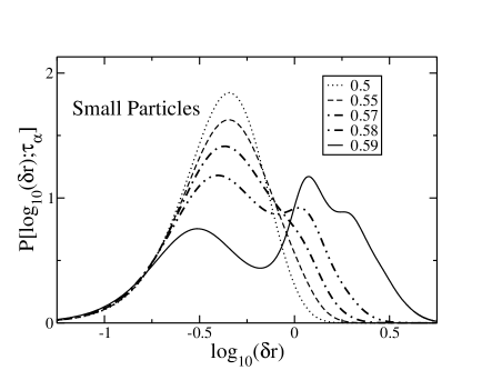
Figure 3: The probability of the logarithm of single particle displacement for the small particles calculated at $\tau_{\alpha}$ for several representative volume fractions. For larger volume fractions there appears a multi-peak structure of $P[\log_{10}(\delta r);t]$ which indicates the existence of sub-populations of slow and fast particles.

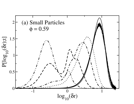
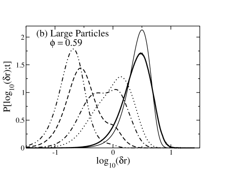
Figure 4: The probability of the logarithm of single particle displacements for $\phi=0.59$ at $0.1\tau_{\alpha}$, $\tau_{\alpha}$, $5\tau_{\alpha}$, $10\tau_{\alpha}$, and $50\tau_{\alpha}$ listed from left to right. The thin solid line is $P[\log_{10}(\delta r);t]$ at $50\tau_{\alpha}$ calculated for a Gaussian distribution of displacements with the same $\left<\delta r^{2}\right>$ as measured in the simulation. (a) small particles. (b) large particles.

To further explore the heterogeneous dynamics we examined the probability of the logarithm of single particles displacements, $P[\log_{10}(\delta r);t]$ at $\tau_{\alpha}$. This probability distribution is related to the self van Hove correlation function, $G_{s}(\delta r;t)=\left<\delta\mathbf{r}-\left[\mathbf{r}_{n}(0)-\mathbf{r}_{n}(t)\right]\right>$, through the relationship $P[\log_{10}(\delta r);t]=\ln(10)4\pi\delta r^{3}G_{s}(\delta r;t)$. The advantage of examining $P[\log_{10}(\delta r);t]$ is that for Fickian diffusion (i.e. for a Gaussian distribution of single particle displacements) its shape is independent of time and its peak value is constant and approximately equal to 2.13 Flenner and Szamel (2005a). Thus, the time-dependence of the shape of $P[\log_{10}(\delta r);t]$ is clear evidence of non-Fickian motion. Furthermore, a multi-peak structure of $P[\log_{10}(\delta r);t]$ is indication of the presence of distinct sub-populations of particles and, thus, heterogeneous dynamics.

Shown in Fig. 3 is $P[\log_{10}(\delta r);\tau_{\alpha}]$ calculated for the small particles at $\phi=0.5$, 0.55, 0.57, 0.58, and 0.59. The behavior is similar to what has been observed in other simulated glass-formers Flenner and Szamel (2005a, b); Reichman et al. (2005); Saltzman and Schweizer (2008) in that multiple peaks emerge close to and at $\phi_{c}$. These peaks correspond to slow and fast particles. In Fig. 4 we show the time dependence of $P[\log_{10}(\delta r);t)]$ for the small particles (a) and large particles (b) for $\phi=0.59$. Shown are times equal to $0.1\tau_{\alpha}$, $\tau_{\alpha}$, $5\tau_{\alpha}$, $10\tau_{\alpha}$, and $50\tau_{\alpha}$. The multiple peaks are evident for both types of particles. The peaks are less pronounced and occur at later times for the large particles.

For long times we would expect the particles to undergo Fickian diffusion. To compare the measured $P[\log_{10}(\delta r);\tau_{\alpha}]$ with those corresponding to Fickian motion we show in Fig. 3 the probability distributions calculated at $50\tau_{\alpha}$ assuming Gaussian distributions of displacements with the same $\left<\delta r^{2}(t)\right>$. It is clear that while for the small particles the difference between the measured distribution and the Fickian one is relatively small, a pronounced difference is observed for the large particles. Thus, even at the relatively long time, $50\tau_{\alpha}$, large particles’ motion is significantly non-Fickian. It should be emphasized that this conclusion cannot be obtained by only investigating the time dependence of the mean square displacement which grows approximately linearly with time on this time scale. Finally, we recall that in an earlier study we showed that in a binary Lennard-Jones system the time scale associated with the onset of Fickian diffusion increases faster with decreasing temperature than the $\alpha$ relaxation time Szamel and Flenner (2006). We expect that a corresponding result, i.e. that the time scale for the onset of Fickian diffusion grows faster with increasing volume fraction than the $\alpha$ relaxation time, holds for the present system.

While one sees clear indications of different sub-populations of slow and fast particles at the higher volume fractions from the results presented in Figs. 3 and 4, one cannot determine how these slow and fast particles are distributed in space. In the next section we examine the spatial correlations amongst the slow particles. As we mentioned in the opening paragraph of the introduction, these particles form clusters and a dynamic correlation length can be associated with the average spatial extent of the clusters.

IV Dynamic Susceptibility and Correlation Length

To examine the spatial extent of the heterogeneous dynamics, we start with a somewhat qualitative approach and look at clusters of slow particles during $\tau_{\alpha}$ utilizing a somewhat arbitrary definition. To visualize these clusters we define the slow particles as those whose displacement $|\mathbf{r}(t)-\mathbf{r}(0)|$ was less than $a=0.3$ over a time $t=\tau_{\alpha}$. We then define two slow particles to be in the same cluster if their initial positions were less than $d_{\alpha\beta}+\Delta_{\alpha\beta}$ apart where $d_{\alpha\beta}=(d_{\alpha}+d_{\beta})/2$ and we used $\Delta_{\alpha\beta}=0.02$. Shown in Fig. 5 are clusters of more than 20 slow particles for $\phi=0.55$ and $\phi=0.59$. It is apparent that the slow particles form clusters; moreover, there are more large clusters at $\phi=0.59$ than at $\phi=0.55$.

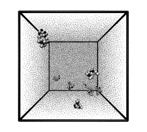
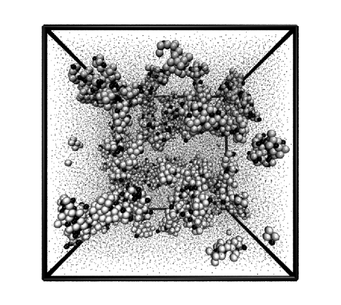
Figure 5: Slow particles’ clusters at $\tau_{\alpha}$ containing more than 20 particles identified using the algorithm described in the text at $\phi=0.55$ (upper figure) and $\phi=0.59$ (lower figure). The white spheres are the large particles, and the black spheres are the small particles. Particles not belonging to the clusters are shown as black dots.

The definition of the clusters shown in Fig. 5 is arbitrary. Alternative definitions results in different clusters. For example, a more common definition uses the separation of the initial positions of slow particles corresponding to the first minimum of the respective pair correlation function,

$$g_{\alpha\beta}(r)=\frac{V}{N_{\alpha}(N_{\beta}-\delta_{\alpha\beta})}\left<\sum_{n}^{N_{\alpha}}\sum_{m\neq n}^{N_{\beta}}\delta(\mathbf{r}-\mathbf{r}_{nm})\right>,$$ (5)

where $V$ is the volume, $r=|\mathbf{r}|$, $\mathbf{r}_{nm}=\mathbf{r}_{n}-\mathbf{r}_{m}$, and the sums are over particles of $\alpha$ and $\beta$ type. Using such a definition we find that the clusters span the entire simulation box. This is not surprising since, by definition, during time $\tau_{\alpha}$ on average 37% of the particles are slow. Thus within the first minimum of $g_{\alpha\beta}(r)$ of a given slow particle another slow particle is likely to be found.

To examine clusters of slow particles somewhat more quantitatively one can generalize the pair correlation functions, Eq. (5), and define a correlation function involving slow particles only,

$$G_{4}(r;t) = \frac{V}{\left<N_{s}(t)\right>(\left<N_{s}(t)\right>-1)}$$

$$\times\left<\sum_{n,m\neq n}w_{n}(t)w_{m}(t)\delta[\mathbf{r}-\mathbf{r}_{nm}(0)]\right>,$$

where microscopic single-particle overlap functions $w_{n}(t)$ select slow particles, and $\left<N_{s}(t)\right>$ is the average number of slow particles, see Eqs. (2-3). Note that the summation in Eq. (IV) is over all, small and large, particles.

The function $G_{4}(r;t)$ is usually referred to as a four-point pair correlation function. Note that by definition, in the thermodynamic limit, $G_{4}(r;t)\to 1$ as $r\to\infty$. By examining $G_{4}(r;t)-1$ we can examine the correlations between slow particles. In particular, the spatial extent of these correlations manifests itself in a slower decay of $G_{4}(r;t)-1$ for large $r$.

Investigation of the extent of the slow particles correlations through a direct analysis of $G_{4}(r)$ is complicated by finite size effects. In particular, in the finite system canonical ensemble the limiting large $r$ value of $G_{4}(r;t)$ differs from 1 by a term inversely proportional to the system size. To correct for this effect in a somewhat quantitative way we determine the large $r$ limit of $G_{4}(r;t)$ by finding the average value of $G_{4}(r;t)-1$ from $r=25.5$ to half the box length and then subtract this average from $G_{4}(r;t)$. The four-point function corrected in this way is denoted by $G_{4}^{c}(r;t)$. This function is shown in Fig. 6. We should emphasize that unlike in some other studies Doliwa and Heuer (2000); Lacevic et al. (2002); Rotman and E. (2010) we do not use this four-point function for a quantitative examination of the slow particles correlations. For the latter task we found it more convenient to analyze the wave-vector dependent analog of $G_{4}(r;t)$.

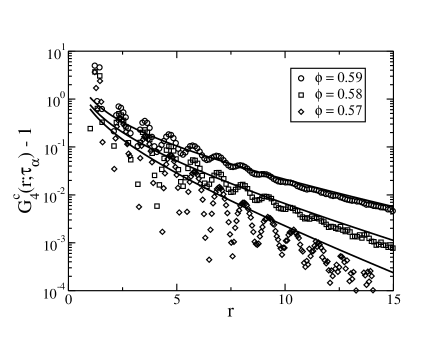
Figure 6: The four-point correlation function $G_{4}^{c}(r;\tau_{\alpha})-1$ for $\phi=$ 0.59, 0.58, and 0.57 listed from top to bottom. The lines are proportional to $\exp[r/\xi(\tau_{\alpha})]/r$ where $\xi(\tau_{\alpha})$ are determined by fits to $S_{4}(q;\tau_{\alpha})$.

Shown in Fig. 6 is $G_{4}^{c}(r;\tau_{\alpha})-1$ for $\phi=0.57$, 0.58, and 0.59. The slower decay for larger $\phi$ is evident, which indicates a larger correlation length associated with the average size of the slow clusters with increasing $\phi$.

To quantitatively determine the spatial extent of correlations of the slow particles we examine the $q$ dependence of the four-point structure factor,

$$S_{4}(q;t) = \frac{\left<N_{s}(t)\right>(\left<N_{s}(t)\right>-1)}{NV}\tilde{G}_{4}(q;t)+\frac{\left<N_{s}(t)\right>}{N}$$

$$= N^{-1}\left(\left<W(\mathbf{q},t)W(-\mathbf{q},t)\right>-\left|\left<W(\mathbf{q};t)\right>\right|^{2}\right),$$

where $W(\mathbf{q};t)$ is the Fourier transform of the spatially resolved microscopic overlap function,

$$W(\mathbf{q};t)=\sum_{n}w_{n}(t)\exp[-i\mathbf{q}\cdot\mathbf{r}_{n}(0)]$$ (8)

and $\tilde{G}_{4}(q;t)$ is the Fourier transform of $G_{4}(r;t)-1$.

In the following two sub-sections we discuss two quantities that can be obtained from the four-point structure factor: the dynamic susceptibility $\chi_{4}(t)$ and the dynamic correlation length $\xi(t)$.

IV.1 Dynamic Susceptibility $\chi_{4}(t)$

The dynamic susceptibility, $\chi_{4}(t)$, is defined as the $q\to 0$ limit of the four-point structure factor,

$$\chi_{4}(t)=\lim_{q\rightarrow 0}S_{4}(q;t).$$ (9)

Since as $\mathbf{q}\to 0$, $W(\mathbf{q};t)\to\sum_{n}w_{n}(t)\equiv N_{s}(t)$ (note that in the preliminary report Flenner and G. (2010) we used $W(t)$ to denote the $\sum_{n}w_{n}(t)$) the dynamic susceptibility measures the ratio of the fluctuation of the number of slow particles to the total number of particles, and we could formally write

$$\chi_{4}(t)=N^{-1}\left(\left<N_{s}^{2}(t)\right>-\left<N_{s}(t)\right>^{2}\right).$$ (10)

It should be emphasized that the right-hand-side of Eq. (10) depends on the ensemble. In the ensemble used in our study the number of particles of both species are kept constant or, alternatively, the volume fraction $\phi$ and the concentration $c$ are kept constant. Thus, hereafter we will denote the right-hand-side of Eq. (10) by $\chi_{4}(t)|_{\phi,c}$,

$$\chi_{4}(t)|_{\phi,c}=N^{-1}\left(\left<N_{s}^{2}(t)\right>-\left<N_{s}(t)\right>^{2}\right)$$ (11)

where it is implicitly understood that the ensemble at the right-hand-side is the constant $\phi$ and $c$ simulational ensemble. It should be noted that while $\chi_{4}(t)|_{\phi,c}$ can be easily calculated in a simulation, in order to determine the ensemble-independent susceptibility $\chi_{4}(t)$ one needs to perform a rather delicate extrapolation procedure $\lim_{q\rightarrow 0}S_{4}(q;t)$.

We note here that the difference between $\chi_{4}(t)|_{\phi,c}$ and $\chi_{4}(t)$ is the reciprocal space manifestation of the finite size and ensemble dependencies of the large $r$ limit of the four-point correlation function $G_{4}(r;t)$.

Berthier et al. Berthier et al. (2005a) pointed out that the susceptibility $\chi_{4}(t)$ can be determined without extrapolating $S_{4}(q;t)$ by using the formalism introduced in Ref. Lebowitz et al. (1967). This procedure results in the following expression

$$\chi_{4}(t) = \chi_{4}(t)|_{\phi,c}+\chi_{\phi}^{2}(t)H_{1}+\chi_{\phi}(t)\chi_{c}(t)H_{2}+\chi_{c}^{2}(t)H_{3}$$ (12)

$$+F_{o}^{2}(t)H_{4}+F_{o}(t)\chi_{\phi}(t)H_{5}+F_{o}(t)\chi_{c}(t)H_{6},$$

where $\chi_{\phi}(t)=\partial F_{o}(t)/\partial\phi$ and $\chi_{c}(t)=\partial F_{o}(t)/\partial c$. The volume fraction dependent, but time independent, quantities $H_{n}$ are linear functions of the partial structure factors $S_{\alpha\beta}(q)$ extrapolated to $q=0$. Note that we changed notation from previous work, Ref. Flenner and G. (2010), where we used $G_{n}$ instead of $H_{n}$.This was done to avoid confusion with the four-point correlation function $G_{4}(r;t)$.

In Appendix B we present a derivation of Eq. 12, give the explicit formulae for the quantities $H_{n}$, and describe how these quantities were evaluated. In the same appendix we also describe an extrapolation procedure that confirmed the consistency of the definition (9) and the expression (12).

It was further argued by Berthier et al. Berthier et al. (2005a) that Eq. (12) could be used to establish an experimental lower bound for $\chi_{4}(t)$. Since $\chi_{4}(t)|_{\phi,c}>0$ the correction terms at the right-hand-side of Eq. (12) constitute a lower bound for $\chi_{4}(t)$. Furthermore, since around the $\alpha$ relaxation time the first correction term is the dominant one, we could neglect all the other terms and thus arrive at

$$\chi_{4}(t)\geq\chi_{\phi}^{2}(t)H_{1}.$$ (13)

If it could be shown that the $\chi_{\phi}^{2}(t)H_{1}$ term dominates close to the glass transition, one would have a simple approximation for the dynamic susceptibility. We start by examining the time and $\phi$ dependence of the terms on the right hand side of Eq. (12) to examine this approximation in detail.

Shown in Fig. 7 is $\chi_{4}(t)|_{\phi,c}$ and all the correction terms given in Eq. (12) for a representative volume fraction $\phi=0.57$. For very short times, the $F_{o}^{2}(t)H_{4}$ term is the largest, as it must be since it is the only term not equal to zero at $t=0$, but it monotonically decays to zero. By the $\beta$ relaxation time, $\chi_{4}(t)|_{\phi,c}$ and the $\chi_{\phi}^{2}(t)H_{1}$ term are the largest, and by the $\alpha$ relaxation time they are around an order of magnitude larger than the other terms. For the volume fraction shown, these two terms are almost equal around $\tau_{\alpha}$, but the $\chi_{\phi}^{2}(t)H_{1}$ term becomes larger at later times.

We note that with increasing volume fraction $\chi_{\phi}^{2}(\tau_{\alpha})H_{1}$ grows faster than $\chi_{4}(\tau_{\alpha})|_{\phi,c}$. The $\chi_{\phi}^{2}(\tau_{\alpha})H_{1}$ term becomes the dominant one for $\phi\geq 0.58$, Fig. 8. This is qualitatively consistent with result of Brambilla et al. Brambilla et al. (2009). The quantitative difference between our Fig. 8 and results shown in Fig. 3a of Ref. Brambilla et al. (2009) originates from the fact that Brambilla et al. systematically overestimated the isothermal compressibility which enters into their correction term.

For our range of volume fractions we do not find that $\chi_{4}(\tau_{\alpha})|_{\phi,c}$ is negligible compared to $\chi_{\phi}^{2}(\tau_{\alpha})H_{1}$. However, for volume fractions larger than the ones examined in this study, it is likely that $\chi_{4}(\tau_{\alpha})$ is well approximated by $\chi_{\phi}^{2}(\tau_{\alpha})H_{1}$ term alone.

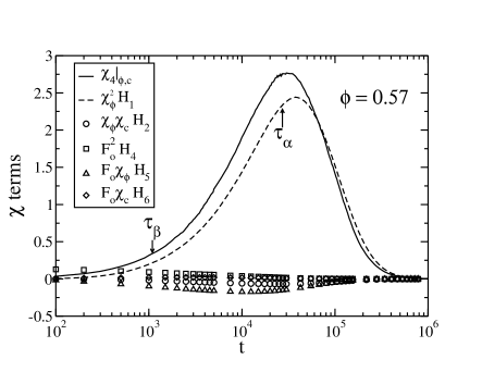
Figure 7: Time dependence of the terms that contribute to $\chi_{4}(t)$ for $\phi=0.57$. The arrow indicate the $\beta$ relaxation time $\tau_{\beta}$ and the $\alpha$ relaxation time $\tau_{\alpha}$.

Figure 8: Volume fraction dependence of the constant $\phi$ and $c$ part of the dynamic susceptibility, $\chi_{4}(\tau_{\alpha})|_{\phi,c}$ (circles), the dominant correction term, $\chi_{\phi}^{2}(\tau_{\alpha})H_{1}$ (triangles), and the ensemble independent susceptibility $\chi_{4}(t)$ calculated from Eq. (12) (open squares).

As can be seen in Fig. 7, around $\tau_{\alpha}$ a good approximation to $\chi_{4}(t)$ is

$$\chi_{4}^{a}(t)=\chi_{4}(t)|_{\phi,c}+\chi_{\phi}^{2}(t)H_{1}.$$ (14)

The time dependence of this quantity is shown in Fig. 9. We observe that $\chi_{4}^{a}(t)$ grows with time, indicating an increase of the overall strength of dynamic heterogeneity, until it reaches a peak that occurs around $\tau_{\alpha}$ and then decreases to zero at later times. The decrease in $\chi_{4}^{a}(t)$ represents a diminishing of the overall strength of the heterogeneous dynamics but the length scale associated with slow clusters do not have to follow the same trends.

Toninelli et al. Toninelli et al. (2005) and Chandler et al. Chandler et al. (2006) examined theoretical predictions for the time dependence of $\chi_{4}(t)$ and compared them with, inter alia particle-based simulations. It is not clear whether the latter comparisons were hindered by fact that global fluctuations were suppressed in simulations. However, in general, a common feature predicted by many theories is a power law growth of $\chi_{4}(t)$ while approaching the peak. This fact prompted us to look for power laws in $\chi_{4}^{a}(t)$.

For smaller volume fractions we do not find any region of power law growth approaching $\tau_{\alpha}$. Around $\phi=0.56$ there emerges a region where $\chi_{4}^{a}(t)$ appears to grow according to a power law, but the exponent in the power law depends on $\phi$. This is due to the two contributions to $\chi_{4}^{a}(t)$ having different magnitudes and time dependencies. For example, for $\phi=0.59$ we find that $\chi_{4}^{a}(t)\sim t^{0.665}$ in the $\alpha$ relaxation regime. This growth is due to a combination of $\chi_{\phi}^{2}(t)\sim t^{0.75}$ and $\chi_{4}|_{\phi,c}\sim t^{0.55}$ in the $\alpha$ relaxation time regime. This analysis suggests that the power law growth of $\chi_{4}^{a}(t)$ does not necessarily have a deeper meaning, at least for volume fractions accessible in our study.

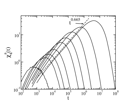
Figure 9: The approximation of the dynamic susceptibility $\chi_{4}^{a}(t)=\chi_{4}(t)|_{\phi,c}+\chi_{\phi}^{2}(t)H_{1}$ for $\phi=0.5$, 0.52, 0.54, 0.55, 0.56, 0.57, 0.575, 0.58, 0.585, and 0.59 listed from left to right. This approximation is accurate around $\tau_{\alpha}$, i.e. around the peak shown in the figure, and becomes increasingly more accurate as $\phi$ increases.

As we remarked above, we expect that for sufficiently high volume fractions the growth of $\chi_{4}(t)$ can be obtained from experiments using the $\chi_{\phi}^{2}(t)H_{1}$ correction term as an approximation for $\chi_{4}(t)$. Moreover, if time-temperature superposition holds, then the growth of $\chi_{\phi}^{2}(t)$ is related to the growth of the $\alpha$ relaxation time. Below, we investigate the consequencies of this idea.

For hard sphere systems, time-temperature superposition is replaced by time-volume fraction superposition. Specifically, the statement is that $F_{o}(t/\tau_{\alpha})$ overlaps in the $\alpha$ relaxation regime when plotted for different $\phi$. We find good overlap for $\phi\geq 0.58$, although we do observe small systematic deviations. Moreover, we find that $F_{o}(t/\tau_{\alpha})$ is well described by a stretched exponential $Ae^{-(t/\tau_{\alpha})^{\beta}}$ (see Fig. 1). Thus, ignoring the weak volume fraction dependence of $A$ and $\beta$ the first correction term in Eq. (12) at $\tau_{\alpha}$ is given by

$$\chi_{\phi}^{2}(\tau_{\alpha})H_{1}=\left(\frac{2A\beta}{(d_{1}^{3}+d_{2}^{3})}\right)^{2}\left(\frac{\partial\ln(\tau_{\alpha})}{\partial\ln(\phi)}\right)^{2}e^{-2}H_{1}.$$ (15)

Recall that this is the largest term for $\phi\geq 0.58$. Since liquid structure is weakly volume-fraction dependent, $H_{1}$ changes slowly with $\phi$. Notice that $A$, $\beta$ and $H_{1}$ are all less than one or equal to one for all $\phi$, and are all less than one for $\phi\geq 0.58$. Note also that $2/(d_{1}^{3}+d_{2}^{3})=0.53419/d_{1}^{3}$. Thus, the coefficient multiplying $[\partial\ln(\tau_{\alpha})/\partial\ln(\phi)]^{2}$ is less than one at all $\phi$ and is very weakly $\phi$ dependent. Consequently, $\chi_{4}(t)$ behaves as $[\partial\ln(\tau_{\alpha})/\partial\ln(\phi)]^{2}$ when the $\chi_{\phi}^{2}$ term is dominant. Finally, since at the largest volume fractions $\tau_{\alpha}=\tau_{\infty}\exp[B/(\phi_{0}-\phi)^{2}]$ provides a good fir to our data, then these arguments indicate that $\chi_{4}(\tau_{\alpha})\sim\phi^{2}(\phi_{0}-\phi)^{-6}$ close to $\phi_{0}$. We find that this indeed provides a good description of our results for the dynamic susceptibility (See Fig. 11).

IV.2 Dynamic Correlation Length $\xi(t)$

To define the dynamic correlation length $\xi(t)$ we need to examine the long wavelength (small wave-vector) behavior of the four-point structure factor. Specifically, we use the following definition of the dynamic correlation length:

$$\xi^{2}(t)=\lim_{q\to 0}q^{-2}\left(\frac{\lim_{k\to 0}S_{4}(k;t)}{S_{4}(q;t)}-1\right).$$ (16)

Definition (16) is consistent with asymptotic small wave-vector Ornstein-Zernicke form of the four-point structure factor,

$$S_{4}(q;t)\approx\frac{\chi_{4}(t)}{1+\xi(t)^{2}q^{2}}\;\mathrm{as}\;q\to 0.$$ (17)

We should note that formally definition (16) is equivalent to defining $\xi(t)$ as the second moment of $G_{4}(r;t)-1$ divided by the zeroth moment of $G_{4}(r;t)-1$. However, we found that the finite size and ensemble effects are easier to account for in the reciprocal space and therefore we used definition (16).

To obtain reliable results for $\chi_{4}(t)$ and $\xi(t)$ we fitted the simulation results to several different functional forms (see Appendix B for details). We determined that the best procedure is to fit $S_{4}(q;t)$, including as $q=0$ value the right-hand-side of Eq. (12), to the Ornstein-Zernicke form while restricting the fitting range to $q<1.5/\xi(t)$. Such fits at $\tau_{\alpha}$ are shown in Fig. 10, for volume fractions $\phi=0.59$, 0.58, 0.57, 0.56, 0.55, 0.52, and 0.50, calculated using the $80\,000$ particle simulations (note the the system size dictates the smallest non-zero wave-vector).

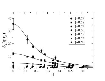
Figure 10: Dynamic structure factor $S_{4}(q;\tau_{\alpha})$ for $\phi=$ 0.59, 0.58, 0.57, 0.56, 0.55, 0.55, 0.52, and 0.50. The values at $q=0$ were calculated using Eq. (12). The lines are Ornstein-Zernicke fits.

Shown in Fig. 11 is the volume fraction dependence of the resulting dynamic susceptibility and correlation length. Note that in this figure we also included results obtained applying the same procedure to data obtained from $10\,000$ particle simulations. The consistency of both sets of results indicates that our procedure can be used to determine the dynamic susceptibility and correlation length using moderately large systems.

We find that the volume fraction dependence of $\xi(\tau_{\alpha})$ can be well described by many different fit functions (the results of the mode-coupling like fits are described in detail in Appendix A). To be consistent with previous fits to $\tau_{\alpha}$ and $D$, we fix $\phi_{c}=0.59$ and fit $\xi(\tau_{\alpha})$ to a mode-coupling like power law, $\xi(\tau_{\alpha})\sim(\phi_{c}-\phi)^{-\gamma_{\xi}}$. This results in $\gamma_{\xi}=0.5\pm 0.1$. The corresponding fit is shown as the dashed line in Fig. 11. The value of $\gamma_{\xi}$ obtained from the fit does not agree with the inhomogeneous mode-coupling prediction of $\gamma_{\xi}=0.25$ Biroli et al. (2006); Szamel and Flenner (2010).

Next we fit $\xi(\tau_{\alpha})$ to $\xi_{0}+C(\phi_{0}-\phi)^{-2}$ over the whole range of $\phi$, which gives $\phi_{0}=0.0635\pm 0.004$ and $\xi_{0}=0.37\pm 0.1$. The corresponding fit is shown as the solid line in Fig. 11, and provides an accurate description of $\xi(\tau_{\alpha})$ for every volume fraction examined in this work. Note that the same $\phi_{0}=0.635$ was obtained from fits of the $\alpha$ relaxation time to the formula suggested by Berthier and Witten Berthier and Witten (2009), $\tau_{\alpha}=\tau_{\infty}\exp[B(\phi_{0}-\phi)^{-2})]$ (see Appendix A). This observation suggests that the following correlation between the $\alpha$ relaxation time and the length, $\tau_{\alpha}=\tau_{0}\exp[k\xi(\tau_{\alpha})]$. We discuss this relationship in Sec. V.

We now look at the scaling relationship between the dynamic susceptibility and the length, $\chi_{4}(\tau_{\alpha})\sim\xi(\tau_{\alpha})^{2-\eta}$. For compact clusters it is expected that $2-\eta=d$ where $d$ is the spatial dimension. Shown in the inset to Fig. 11 is the scaling fit for $\phi\geq 0.56$. We obtain $2-\eta=2.9\pm 0.1$, which indeed suggests compact clusters. The comparison of this result with the inhomogeneous mode-coupling theory prediction Biroli et al. (2006); Szamel and Flenner (2010) is a little involved. The theory analyzes a three-point susceptibility and finds that in the $\alpha$ relaxation regime $\lim_{\mathbf{q}\to 0}\chi_{3}(\mathbf{q};\tau_{\alpha})\sim\xi(\tau_{\alpha})^{4}$. Field-theoretical considerations Berthier et al. (2007a, b) indicate that the dynamic susceptibility is a quadratic function of the three-point susceptibility. A combination of both results would suggest a prediction $\chi_{4}(\tau_{\alpha})\sim\xi(\tau_{\alpha})^{8}$ which is clearly well outside the simulational result.

Since we find that $\xi(\tau_{\alpha})=\xi_{0}+C(\phi_{0}-\phi)^{-2}$ provides a good description of all the data and that $\chi_{4}(\tau_{\alpha})\approx a_{4}\xi(\tau_{\alpha})^{3}$ for $\phi\geq 0.55$, we show $a_{4}[\xi_{0}+C(\phi_{0}-\phi)^{-2}]^{3}$ as the solid line through $\chi_{4}(\tau_{\alpha})$ in Fig. 11. Note that this is not an independent fit. However, it describes the data fairly well over the whole range of studied volume fractions. Moreover, it is consistent with the limiting behavior $\chi_{4}(\tau_{\alpha})\sim\phi^{2}(\phi_{0}-\phi)^{-6}$ obtained from the first correction in Eq. (12).

In Fig. 11 we also show, as a dashed line, the third power of the mode coupling fit. As expected, it gives a reasonable description of the data between $0.55\leq\phi\leq 0.58$.

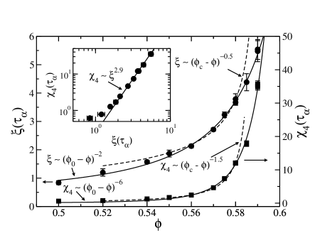
Figure 11: The dynamic correlation length $\xi(\tau_{\alpha})$ versus $\phi$ (left axis) and the dynamic susceptibility $\chi_{4}(\tau_{\alpha})$ versus $\phi$ (right axis). The solid line through $\xi(\tau_{\alpha})$ is a fit to $\xi(\tau_{\alpha})=\xi_{0}+A(\phi_{0}-\phi)^{-2}$ where $\phi_{0}=0.635$. The dashed line through $\xi(\tau_{\alpha})$ is a mode-coupling like fit $\xi(\tau_{\alpha})\sim(\phi_{c}-\phi)^{-\gamma_{\xi}}$ where $\phi_{c}=0.59$ is fixed and we obtain $\gamma_{\xi}=0.5\pm 0.1$. In the inset we show $\chi_{4}(\tau_{\alpha})$ versus $\xi(\tau_{\alpha})$, and we find that $\chi_{4}(\tau_{\alpha})\sim\xi(\tau_{\alpha})^{2.9}$ for $\phi\geq 0.55$.

We now examine the time dependence of the dynamic correlation length. Shown in Fig. 12 is $\xi(t)$ versus time for different $\phi$. For all $\phi$, the dynamic correlation length grows with time and then plateaus at later times, and remains constant up to the maximum time at which we can evaluate it. We cannot accurately calculate $\xi(t)$ for $t\gtrsim 10\tau_{\alpha}$ because there are few slow particles at such long times. Thus, we do not know the fate $\xi$ at later times.

We note that one previous simulational investigation of the time dependence of the dynamic correlation length resulted in length whose time dependence roughly follows that of the dynamic susceptibility Lacevic et al. (2003). A different study found a monotonically increasing dynamic correlation length Toninelli et al. (2005). On the other hand, an earlier study Doliwa and Heuer (2000), which used a somewhat different definition of the dynamic correlation length, found that the length was increasing with time but then plateaued after $\tau_{\alpha}$. A similar behavior was found in a very recent study of a two-dimensional lattice gas glassy system Rotman and E. (2010). The two latter results are (at least qualitatively) consistent with our findings.

We remark that a plateau in the time dependence of a characteristic dynamic length is predicted by the inhomogeneous mode-coupling theory Biroli et al. (2006); Szamel and Flenner (2010). However, the plateau predicted by this theory occurs around the $\beta$ relaxation time, and not after the $\alpha$ relaxation time as seen here.

There are two somewhat surprising features in the results shown in Fig. 12. First, for $\phi\geq 0.56$ and between $\tau_{\beta}$ and $\tau_{\alpha}$, the dynamic correlation length is independent of the volume fraction and only depends on time. We don’t have sufficient data for times smaller than the $\beta$ relaxation time, but we expect that this universal behavior breaks down at short times. The correlation length appears to follow a master curve until it reaches a volume fraction dependent asymptotic value, which we will refer to $\xi_{\mathrm{max}}$. We find that this master cure can be well described by $\xi(t)=a\ln(bt)$, and this fit is shown as a solid line in Fig. 12.

Second, we find that the time at which $\xi(t)$ saturates, which we denote as $\tau_{\mathrm{max}}$, exceeds the $\alpha$ relaxation time and the time at which $\chi_{4}(t)$ peaks, $\tau_{\mathrm{peak}}$ (we find that $\tau_{\alpha}$ and $\tau_{\mathrm{peak}}$ have the same volume fraction dependence). Thus, the dynamic correlation length seems to be growing further while the overall strength of dynamic heterogeneity, measured by the susceptibility, is decreasing. This somewhat surprising finding means that, while at longer time scales there are few slow particles, the characteristic size of the clusters of these particles seems to be constant (at least up to $10\tau_{\alpha}$).

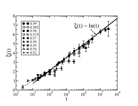
Figure 12: The dynamic correlation length versus time for $\phi\geq 0.52$. The correlation length appears to follow a universal curve until it reaches a volume fraction dependent maximum value, and then it stays approximately constant at later times. The straight line is a fit to the data, $\xi(t)=a\ln(bt)$.

Since $\tau_{\mathrm{max}}$ exceeds $\tau_{\alpha}$, it is obvious that $\xi_{\mathrm{max}}$ exceeds $\xi(\tau_{\alpha})$. Interestingly, there seems to be a linear relationship between these two lengths, Fig. 13. Combining the linear relationship between $\xi_{\mathrm{max}}$ and $\xi(\tau_{\alpha})$ with the previous observation that $\xi(t)=a\ln(bt)$, we see that $\tau_{\mathrm{max}}\sim\tau_{\alpha}^{\epsilon}$ and through the fits of $\xi_{\mathrm{max}}$ we determine $\epsilon=1.3\pm 0.1$.

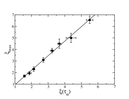
Figure 13: The plateau value $\xi_{\mathrm{max}}$ versus $\xi(\tau_{\alpha})$. The solid line is a linear fit.

The time dependence of the dynamic correlation length shown in Fig. 12 suggests that possibly we should focus more on the plateau value of the dynamic correlation length, $\xi_{\mathrm{max}}$, than on the length at the $\alpha$ relaxation time, $\xi(\tau_{\alpha})$. This suggestion is left for future investigation.

V correlation length and average dynamics

In this section we examine the relationships between the dynamic correlation length $\xi(\tau_{\alpha})$ and the two simplest quantities characterizing the average dynamics, the relaxation time, $\tau_{\alpha}$, and the self-diffusion coefficient, $D$. We note that most theoretical descriptions of glassy dynamics focus on the temperature dependence of the dynamics. Consequently, relationships between $\xi(\tau_{\alpha})$, $\tau_{\alpha}$ and $D$ involve temperature. However, temperature is not a relevant control variable for our hard sphere system. Instead, the volume fraction is the usual control parameter and, therefore, in formulae discussed below we omitted temperature.

We begin by examining the relationship between $\xi(\tau_{\alpha})$ and $\tau_{\alpha}$. The mode-coupling theory predicts a power law $\tau_{\alpha}\sim\xi(\tau_{\alpha})^{z}$. In contrast, the Adam-Gibbs Adam and Gibbs (1965) and Random-First-Order-Transition theories Kirkpatrick et al. (1989) predict an exponential dependence of the relaxation time on a correlation length, $\xi_{s}$, describing the size of cooperatively rearranging regions, $\tau_{\alpha}\sim\exp(\xi_{s}^{\theta})$ where $\theta=3$ in the Adam-Gibbs theory and is a parameter in the Random-First-Order-Transition theory. While it is currently unclear if our dynamic correlation length is the same as the correlation length in Adam-Gibbs and Random-First-Order-Transition theories (in particular our length depends on time whereas $\xi_{s}$ does not have an obvious time dependence) we examine relationships between $\xi$ and $\tau_{\alpha}$ suggested by those theories.

We find that a power law describes well the correlation between $\xi(\tau_{\alpha})$ and $\tau_{\alpha}$ over the mode-coupling regime with $z=4.8\pm 0.3$, see Fig. 14. This exponent disagrees with the inhomogeneous mode-coupling theory prediction of $z\approx 10$ Biroli et al. (2006); Szamel and Flenner (2010) and with some of the previous simulational studies Lacevic et al. (2003); Stein and Andersen (2008), but it is consistent with other previous simulational investigations Whitelam et al. (2004); Flenner and Szamel (2009); Karamakar et al. (2009) (note that in majority of earlier studies the inverses of the exponent $z$ was given).

We find, however, that an exponential dependence of $\tau_{\alpha}$ on $\xi(\tau_{\alpha})$ provides a better description of the data over a larger range of volume fractions. A fit to $\tau_{\alpha}=\tau_{0}\exp(k_{\tau}\xi(\tau_{\alpha})^{\theta})$ gives $\theta=1.1\pm 0.2$. Thus, we fix $\theta=1.0$ and fit $\tau_{\alpha}=\tau_{0}\exp(k_{\tau}\xi(\tau_{\alpha}))$, which is shown as a solid line in Fig. 14. Note that the quality of the latter fit is fully consistent with the fact that independent fits $\tau_{\alpha}=\tau_{\infty}\exp[B(\phi_{0}-\phi)^{-2}]$ and $\xi(\tau_{\alpha})=\xi_{0}+C(\phi_{0}-\phi)^{-2}$ result in the same value $\phi_{0}=0.635$ (see Appendix A).

In Fig. 14 we also show $1/D$ versus $\xi(\tau_{\alpha})$. The results do not seem to follow a straight line and thus we do not find that $D\sim\exp(-k_{D}\xi(\tau_{\alpha}))$, but rather $D=D_{0}\exp(-k_{D}\xi(\tau_{\alpha})^{\theta})$ where $\theta=0.61\pm 0.04$. The latter fit is shown as a solid line in the figure. Again, we note that the quality of the self-diffusion coefficient fit is quite good. However, we shall also note that a combination of both correlations $\tau_{\alpha}=\tau_{0}\exp(k_{\tau}\xi(\tau_{\alpha}))$ and $D=D_{0}\exp(-k_{D}\xi(\tau_{\alpha})^{\theta})$ is, strictly speaking, not compatible with a power-law relationship between the self-diffusion coefficient and the relaxation time discussed in Sec. III

Finally, we briefly mention two other, different investigations that analyzed somewhat different characteristic dynamic lengths.

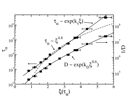
Figure 14: The alpha relaxation time $\tau_{\alpha}$ and the diffusion coefficient $D$ as a function of $\xi(\tau_{\alpha})$. The solid straight line is an exponential fits to the relaxation time data $\tau_{\alpha}\sim\exp[\xi(\tau_{\alpha})]$ and the solid curved line is a fit $1/D\sim\exp[\xi(\tau_{\alpha})^{\theta}]$ with $\theta=0.6$. The dashed line is a mode-coupling theory like fit to $\tau_{\alpha}\sim\xi(\tau_{\alpha})^{z}$ with $z=4.8$.

Saltzman and Schweizer Saltzman and Schweizer (2006a, b); Saltzman and Schweizer (2008) investigated a characteristic length associated with the onset of Fickian diffusion. They showed that this length, $\xi_{D}$, depends logarithmically on the relaxation time, $\xi_{D}\sim\ln(\tau_{\alpha})$. This result is consistent with our relation between the dynamic correlation length at the $\alpha$ relaxation time and the $\alpha$ relaxation time.

A similar crossover length was examined in models of facilitated dynamics Berthier et al. (2005b). Berthier et al. defined a length scale associated with the onset of Fickian diffusion as $\ell^{*}\sim\sqrt{D\tau_{\alpha}}$. They noted that $\ell^{*}\sim\tau_{\alpha}^{(1-\sigma)/2}$ where $\sigma$ is the dynamic exponent describing the violation of the Stokes-Einstein relation. Thus, for our system one would expect $\ell^{*}\sim\tau_{\alpha}^{0.2}$. We do find that for our system the relation $\sqrt{D\tau_{\alpha}}\sim\tau_{\alpha}^{0.2}$ is obeyed for large $\tau_{\alpha}$. However, the length $\ell^{*}$ has different volume fraction (or relaxation time) dependence from our dynamic correlation length $\xi(\tau_{\alpha})$. This is qualitatively consistent with the fact that the analysis of facilitated models suggests that the length $\ell^{*}$ is actually different from a dynamic heterogeneity length $\xi$. For example, for the so-called East model, one finds the following relation between the dynamic heterogeneity length and the $\alpha$ relaxation time, $\xi\sim\exp\{\sqrt{\ln(\tau_{\alpha})}\}$ Gar . This relation, for our range of correlation lengths and relaxation times, provides as good fit to our data as the logarithmic relation $\xi(\tau_{\alpha})\sim\ln(\tau_{\alpha})$ discussed above.

VI Discussion

We presented a new computational method to calculate a dynamic correlation length $\xi(t)$ characterizing the spatial extent of heterogeneous dynamics on time scale $t$ and used this new method to obtain a number of results pertaining to dynamic heterogeneity.

Our method combines direct simulational evaluation of the four-point structure factor $S_{4}(q;t)$ for non-zero wave-vectors with an independent calculation of the dynamic susceptibility $\chi_{4}(t)$ that accounts for fluctuations suppressed in the simulational ensemble via procedures derived by Lebowitz et al. Lebowitz et al. (1967). Using the independently obtained dynamic susceptibility as the $q\to 0$ limit of $S_{4}(q;t)$ facilitates analyzing the small $q$ behavior of the four-point structure factor. We found that an Ornstein-Zernicke fits worked well if we restricted our fits such that $q<1.5/\xi(t)$. This procedure allows one to evaluate the dynamic correlation length from simulations of moderately large systems. We also found that the calculation of $\xi(t)$ from the direct space four-point correlation function $G_{4}(r;t)$ is difficult due to the difficult to account for finite size and ensemble dependencies.

We studied the volume fraction and the time dependence of the dynamic correlation length. We also explored relationships between the length, the dynamic susceptibility, and quantities characterizing the average dynamics, the $\alpha$ relaxation time and the self-diffusion coefficient.

First, we found that $\xi(\tau_{\alpha})\sim(\phi_{0}-\phi)^{-2}$ provides a good description of the data. We note, however, $\xi(\tau_{\alpha})$ can also be fitted by other functions. We also found that mode-coupling like power law $\xi(\tau_{\alpha})\sim(\phi_{c}-\phi)^{-\gamma_{\xi}}$ provides a good description of $\xi(\tau_{\alpha})$ for the mode-coupling theory range of volume fractions, but the exponent $\gamma_{\xi}=0.5$ differs from the inhomogeneous mode-coupling theory prediction of $\gamma_{\xi}=0.25$ Biroli et al. (2006); Szamel and Flenner (2010).

Next, we studied the time dependence of $\chi_{4}(t)$ and $\xi(t)$. While we did find a power law dependence on time, $\chi_{4}(t)\sim t^{c}$, for times around the $\alpha$ relaxation time, the exponent $c$ was volume fraction dependent and decreased with increasing $\phi$. Surprisingly, we found that for a range of times between the $\beta$ and $\alpha$ relaxation times the dynamic correlation length followed a master curve independent of $\phi$ until it reached a volume fraction dependent plateau value. The dependence of $\xi(t)$ on time could be fitted with a simple $\xi(t)\sim\ln(t)$ relation. The plateau value, $\xi_{\mathrm{max}}$, was reached at a characteristic time, $\tau_{\mathrm{max}}$. We found that $\tau_{\mathrm{max}}$ exceeds and grows faster with increasing volume fraction than the $\alpha$ relaxation time.

We examined the correlations between $\xi(\tau_{\alpha})$, $\tau_{\alpha}$, and $D$, and we found that mode-coupling like power law fits provide a good description of the data for $0.55\leq\phi\leq 0.58$. We found deviations from these fits as $\phi_{c}=0.59$ is approached. While the mode-coupling exponents for $\tau_{\alpha}$ and $D$ agree reasonably well with the mode-coupling predictions, the exponents for $\xi(\tau_{\alpha})$ and $\chi_{4}(\tau_{\alpha})$ do not. We also find that $\chi_{4}(\tau_{\alpha})\sim\xi(\tau_{\alpha})^{3}$, which does not agree with the inhomogeneous mode coupling prediction.

Finally, we found that an exponential dependencies of the $\alpha$ relaxation time and the self-diffusion coefficient on the dynamic correlation length evaluated at the $\alpha$ relaxation time, $\tau_{\alpha}\sim\exp(\xi(\tau_{\alpha}))$ and $D\sim\exp(-\xi(\tau_{\alpha})^{0.6})$, describe our data well. This is consistent with the spirit of Adam-Gibbs and Random-First-Order-Transition theories. The values of the scaling exponents are inconsistent with the traditional Adam-Gibbs picture where the relaxation, either $\tau_{\alpha}$ or $1/D$, behaves as $\exp(\xi_{s}^{3})$. Note, however, that Adam-Gibbs and Random-First-Order-Transition theories are formulated in terms of the characteristic size of dynamically correlated regions, $\xi_{s}$ whereas we calculated and examined the dynamic correlation length. Further work is required to clarify the connection between these lengths.

VII Acknowledgments

We gratefully acknowledge the support of NSF Grant No. CHE 0909676.

Appendix A Characteristic Volume Fractions

To test theories of the glass transition it is common to fit experimental and simulation data to different functions. The quality of the fits can vary depending on the range used for the fits and the proximity to any singularity implied by the fitting function. In this section we examine some commonly used fitting functions to various $\phi$ dependent quantities, a mode-coupling like fit $(\phi_{c}-\phi)^{-\gamma}$, a Vogel-Fucher-Tamman (VFT) like form $\exp[A(\phi_{VF}-\phi)^{-1}]$ and a form suggested by Berthier and Witten (BW), $\exp[B(\phi_{0}-\phi)^{-2}]$ Berthier and Witten (2009). The mode-coupling fits are used to determine a range of volume fractions where the mode-coupling like power laws provide a good description of the data. We use this range of $\phi$ to compare our simulation results to the predictions of the mode-coupling theory and the inhomogeneous mode-coupling theory. Outside of this range we do not expect the mode-coupling theory to provide a very good description of the dynamics. The goal of this appendix is to examine our results and previous arguments in the literature to find the best unified description of the data. To achieve this goal, we not only examine our data, but also use results from earlier investigationsOdriozola and Berthier (2010); Berthier and Witten (2009).

First we examine mode-coupling like fits to the $\alpha$ relaxation time $\tau_{\alpha}$ and the self-diffusion coefficient $D$. The mode-coupling theory predicts a power law divergence of $\tau_{\alpha}$ and a power law vanishing of $D$ with the same exponent $\gamma$. It has been found in several numerical studies of the mode-coupling theory that $\gamma\approx 2.46$ Flenner and Szamel (2005b); Szamel and Flenner (2010). One of the difficulties in performing these fits is that, while the mode-coupling theory predicts that Stokes-Einstein relation is obeyed, $\tau_{\alpha}D=\mathrm{const.}$, Flenner and Szamel (2005b), this relation is violated in simulations and experiments. Importantly, in most simulations the violation of the Stokes-Einstein relation is apparent already in the regime in which power law fits are applicable. Thus, the best one can do is to use different exponents for $\tau_{\alpha}$ and $D$ and the same mode-coupling transition volume fraction or temperature. A seemingly worse alternative is to force the same exponent and obtain two different mode coupling transition points.

We fit $\tau_{\alpha}$, $1/D$, $\xi(\tau_{\alpha})$, and $\chi_{4}(\tau_{\alpha})$ to power laws of the form $a(\phi_{c}-\phi)^{-\gamma}$ for $0.55\leq\phi\leq 0.575$ and $0.55\leq\phi\leq 0.58$. The results are summarized in Table 1. We find that $\phi_{c}$ varies from $0.58$ to 0.61, but a consistent value is around $\phi_{c}\approx 0.59$. Since $\phi_{c}=0.59$ is consistent with our results, has been used in the literature previously Brambilla et al. (2009), and coincides with the onset of ”hopping” like motion observed in Sec. III, we fix $\phi_{c}=0.59$ in this work. We also identify $0.55\leq\phi\leq 0.58$ as the mode-coupling regime, but this should be considered as only an approximate regime where the mode-coupling theory provides a reasonable description of the data.

Having chosen a common value for the mode-coupling transition volume fraction we redo the fits for $1/D$, $\tau_{\alpha}$, $\chi_{4}(\tau_{\alpha})$, and $\xi(\tau_{\alpha})$ keeping $\phi_{c}=0.59$ fixed. The fit parameters are the bottom set in Table 1.

Table 1: Fits to a mode-coupling like power law over different ranges of volume functions. The number in parenthesis represents the uncertainty in the last digit. The bottom set of data is with $\phi_{c}=0.59$ fixed.

variable	$\phi_{c}$	$\gamma$	fit range
$\tau_{\alpha}$	$0.5874(4)$	$2.21(6)$	$0.55\leq\phi\leq 0.575$
$D$	$0.5911(7)$	$2.13(6)$	$0.55\leq\phi\leq 0.575$
$\chi_{4}(\tau_{\alpha})$	$0.58(4)$	$1.3(2)$	$0.55\leq\phi\leq 0.575$
$\xi(\tau_{\alpha})$	$0.586(4)$	$0.47(9)$	$0.55\leq\phi\leq 0.575$
$\tau_{\alpha}$	$0.5901(6)$	$2.47(6)$	$0.55\leq\phi\leq 0.58$
$D$	$0.5950(4)$	$2.42(5)$	$0.55\leq\phi\leq 0.58$
$\chi_{4}(\tau_{\alpha})$	$0.593(3)$	$1.7(2)$	$0.55\leq\phi\leq 0.58$
$\xi(\tau_{\alpha})$	$0.61(2)$	$0.9(4)$	$0.55\leq\phi\leq 0.58$
$\tau_{\alpha}$	$0.59$	$2.43(1)$	$0.55\leq\phi\leq 0.58$
$D$	$0.59$	$1.94(3)$	$0.55\leq\phi\leq 0.58$
$\chi_{4}(\tau_{\alpha})$	$0.59$	$1.46(4)$	$0.55\leq\phi\leq 0.58$
$\xi(\tau_{\alpha})$	$0.59$	$0.50(3)$	$0.55\leq\phi\leq 0.58$

We now look at the fate of the system beyond the mode-coupling regime. To this end we examine the results of fits to a VFT like functions and a BW like function for $\tau_{\alpha}$. We do not fit other variables since we do are not sure whether the same functions can be used. Note, however, that $\xi(\tau_{\alpha})$ is closely tied to $\tau_{\alpha}$, thus we expect that fits to $\xi(\tau_{\alpha})$ result in the same conclusions.

A fit to $\ln(\tau_{\alpha})=\ln(\tau_{V})+A(\phi_{V}-\phi)^{-1}$ gives $\phi_{V}=0.6122\pm 0.0005$, $\tau_{V}=140\pm 7$ and $A=0.222\pm 0.005$ where we fit $0.55\leq\phi\leq 0.5905$. Next we fit $\ln(\tau_{\alpha})=\ln(\tau_{0})+B(\phi_{0}-\phi)^{-2}$, which gives $\tau_{0}=456\pm 37$, $B=0.017\pm 0.001$, and $\phi_{0}=0.635\pm 0.002$. Shown in Fig. 15 are these fits along with the results obtained by fitting $\xi(\tau_{\alpha})=\xi_{0}+C(\phi_{0}-\phi)^{-2}$ and then using $\tau_{\alpha}\sim\exp(k\xi)$, which we refer to as the correlation length fit. The VFT fit is the best fit over the largest range of $\phi$, thus one would choose this fit based on the fit quality alone. However, the VFT fit results in a critical volume fraction that appears to be too small when compared with earlier results from the literature.

One result is the dynamic scaling argument of Berthier and Witten Berthier and Witten (2009) who found $\phi_{0}=0.635\pm 0.005$ and $\tau_{\alpha}\sim\exp[B(\phi_{o}-\phi)^{-\delta}]$ with $\delta=2.2\pm 0.2$. This is in remarkable agreement with our fits to $\tau_{\alpha}$ and $\xi(\tau_{\alpha})$. Another is the work of Odriozola and Berthier Odriozola and Berthier (2010) who found no evidence of a thermodynamic transition for $\phi<0.63$ by utilizing a replica exchange Monte Carlo algorithm to examine the equation of state. Finally, we find that $\tau_{\alpha}\approx 5\times 10^{8}$ for a $1\,000$ particle simulation at $\phi=0.6$. This value agrees well with the BW fit that gives $4.85\times 10^{8}$ for $\phi=0.6$, but is orders of magnitude different than the prediction of the VFT fit, $1.1\times 10^{10}$ for $\phi=0.6$. While we expect a $1\,000$ particle system to be too small for $\phi=0.6$ and, in particular, we expect that at this volume fraction $\xi(\tau_{\alpha})$ is larger than half of the $1\,000$ particle system simulation cell, this result does provide some evidence for the BW fit. However, large, fully equilibrated simulations at $\phi$ larger than those utilized in our simulations are needed to test the proper functional form of the divergence.

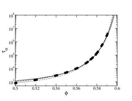
Figure 15: Various fits to $\tau_{\alpha}$ described in the text. The dotted line is a combination of the fit $\xi(\tau_{\alpha})\sim(\phi_{0}-\phi)^{-2}$ and the correlation $\tau_{\alpha}\sim\exp[k\xi(\tau_{\alpha})]$. The dashed line is the Vogel-Fucher-Tamman fit and the solid line is a fit to $\tau_{\alpha}\sim\exp[B(\phi_{0}-\phi)^{-2}]$.

We should emphasize here that our simulations cover both the mode-coupling-like regime and a new regime in which the data are consistent with $\ln(\tau_{\alpha})\sim(\phi_{0}-\phi)^{-2}$.

Appendix B Calculation of $\chi_{4}(t)$ and $\xi(t)$

Here we describe the details of the calculation of the dynamic susceptibility $\chi_{4}(t)$ and the dynamic correlation length $\xi(t)$. The outline of this appendix is as follows. First, we present a derivation of Eq. (12). Next, we show that $\chi_{4}(t)$ calculated from this equation agrees with an independent extrapolation of $S_{4}(q;t)$ to $q=0$. Finally, we use $\chi_{4}(t)$ calculated from formula  (12) as the point at $S_{4}(q=0;t)$ in a fitting procedure to find the most reliable result for the dynamic susceptibility and the dynamic correlation length.

In our simulation, the volume fraction and the concentration of particles is fixed. Thus, fluctuations of the volume fraction and concentration do not contribute to the direct calculation of the dynamic susceptibility. To account for these fluctuations we follow the procedure introduced by Lebowitz et al. Lebowitz et al. (1967). We start by considering an ensemble where the number of particles can fluctuate and calculate the first order corrections to $\chi_{4}(t)$ calculated in an ensemble where the volume fraction and the concentration are held constant. Consider

$$\chi_{4}(t)=$$

$$\frac{1}{\left<N\right>_{(\mu_{1},\mu_{2},V)}}\left<\delta\left(\sum_{n}w_{n}(t)\right)\delta\left(\sum_{m}w_{m}(t)\right)\right>_{(\mu_{1},\mu_{2},V)},$$

where $\left<\right>_{\mathbf{X}}$ denotes an ensemble where $\mathbf{X}$ is held constant. In Eq. B the chemical potentials of both small and large particles, $\mu_{1}$ and $\mu_{2}$, and the volume ($V$) are held constant, but the numbers of particles, $N_{1}$ and $N_{2}$, are allowed to fluctuate. Since the volume is held constant in all the ensembles considered, we will not explicitly indicate the constant $V$ in what follows. According to Eq. 2.11 of Lebowitz et al. Lebowitz et al. (1967),

$$\left<N\right>_{\mu_{1},\mu_{2}}\chi_{4}(t) = \left<\delta\left(\sum_{n}w_{n}(t)\right)\delta\left(\sum_{m}w_{m}(t)\right)\right>_{N_{1},N_{2}}$$ (19)

$$+\left<(\delta N_{1})^{2}\right>_{\mu_{1},\mu_{2}}\left[\frac{\partial\left<\sum_{n}w_{n}\right>_{N_{1},N_{2}}}{\partial N_{1}}\right]^{2}$$

$$+\left<(\delta N_{2})^{2}\right>_{\mu_{1},\mu_{2}}\left[\frac{\partial\left<\sum_{n}w_{n}\right>_{N_{1},N_{2}}}{\partial N_{2}}\right]^{2}$$

$$+2\left<\delta N_{1}\delta N_{2}\right>_{\mu_{1},\mu_{2}}$$

$$\times\frac{\partial\left<\sum_{n}w_{n}\right>_{N_{1},N_{2}}}{\partial N_{1}}\frac{\partial\left<\sum_{n}w_{n}\right>_{N_{1},N_{2}}}{\partial N_{2}}.$$

We utilize the relationship

$$\left<N\right>_{\mu_{1},\mu_{2}}^{-1}\left<\delta N_{n}\delta N_{m}\right>_{\mu_{1},\mu_{2}} = \lim_{q\rightarrow 0}\sqrt{x_{n}x_{m}}S_{nm}(q)$$ (20)

$$= \sqrt{x_{n}x_{m}}S_{nm},$$

where $S_{nm}(q)$ is the partial structure factor and $x_{n}=N_{n}/N$. We also recognize that $\left<\sum_{n}w_{n}(t)\right>_{N}=(N_{1}+N_{2})F_{o}(t)$. Finally, we replace the differentiation with respect to the numbers of particles with the differentiation with respect to the volume fraction and the concentration and in this way we obtain

$$\chi_{4}(t) = \chi_{4}(t)_{N}+\chi_{\phi}^{2}H_{1}+\chi_{\phi}\chi_{c}H_{2}+\chi_{c}^{2}H_{3}$$

$$+F_{o}(t)^{2}H_{4}+F_{o}(t)\chi_{\phi}H_{5}+F_{o}(t)\chi_{c}H_{6},$$

where $\chi_{x}=\partial F_{o}(t)/\partial x$. The $H_{n}$ are functions of $S_{nm}$, and are given by

$$H_{1} = \left(\frac{\pi\rho}{6}\right)^{2}\left[d_{1}^{6}x_{1}S_{11}+2d_{1}^{3}d_{2}^{3}\sqrt{x_{1}x_{2}}S_{12}+d_{2}^{6}x_{2}S_{22}\right]$$

(22)

$$H_{2} = \frac{\pi\rho}{3}\left[d_{1}^{3}x_{1}x_{2}S_{11}-d_{1}^{3}x_{1}\sqrt{x_{1}x_{2}}S_{12}\right.$$ (23)

$$\left.+d_{2}^{3}x_{2}\sqrt{x_{1}x_{2}}S_{12}-d_{2}^{3}x_{1}x_{2}S_{22}\right]$$

$$H_{3} = x_{2}^{2}x_{1}S_{11}-2x_{1}x_{2}\sqrt{x_{1}x_{2}}S_{12}+x_{1}^{2}x_{2}S_{22}$$ (24)

$$H_{4} = x_{1}S_{11}+2\sqrt{x_{1}x_{2}}S_{12}+x_{2}S_{22}$$ (25)

$$H_{5} = \frac{\pi\rho}{3}\left[d_{1}^{3}x_{1}S_{11}+(d_{1}^{3}+d_{2}^{3})\sqrt{x_{1}x_{2}}S_{12}+d_{2}^{3}x_{2}S_{22}\right]$$

$$H_{6} = 2\left[x_{1}x_{2}S_{11}+(x_{2}-x_{1})\sqrt{x_{1}x_{2}}S_{12}-x_{1}x_{2}S_{22}\right].$$

To calculate $H_{n}$ we fit the wave vector dependent version of $H_{n}$, i.e. expressions (22)-(LABEL:H6) with $S_{nm}$ replaced by $S_{nm}(q)$, to a wave-vector independent constants for $q\leq 0.6$. Due to noise in our data we cannot perform a more accurate extrapolation. We checked this approach by using the same procedure to calculate the pressure using the partial structure factors. We checked that the pressure obtained from the $q\to 0$ limit of the structure factors agrees with the pressure obtained from the extrapolation of the pair correlation function to contact.

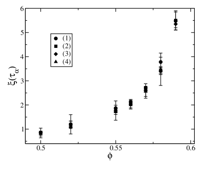
Figure 16: The dynamic correlation length $\xi(\tau_{\alpha})$ obtained using the different fitting procedures described in the text. The number correspond to the different fitting procedures.

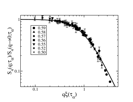
Figure 17: Scaling plot $S_{4}(q;\tau_{\alpha})/S_{4}(q\to 0;\tau_{\alpha})$ versus $q\xi(\tau_{\alpha})$ for the $80\,000$ particle simulations.

To verify Eq. (19) and to check its accuracy, we extrapolated $S_{4}(q;t)$ to $q\rightarrow 0$ by fitting $S_{4}(q;t)$ obtained for non-zero wave-vectors to an Ornstein-Zernicke function. We compared the resulting $\lim_{q\to 0}S_{4}(q;t)$ to $\chi_{4}(t)$ obtained from Eq. (19). The extrapolation agreed to within error and thus we concluded that Eq. (19) provided a good means to calculate $\chi_{4}(t)$. Subsequently, we used Eq. (19) as the $q=0$ value of $S_{4}(q;t)$ in fitting procedures.

It is important to recognize that the above described verification of Eq. (19) requires a rather large system size. In particular, we could only perform it using $N=80\,000$ particles system. Once using $\chi_{4}(t)$ obtained from Eq. (19) as the $q=0$ value of $S_{4}(q;t)$ is accepted, we were able to use moderately large systems ($N=10\,000$ particles).

We fit $S_{4}(q;t)$, using Eq. (19) as the $q=0$ value of $S_{4}(q;t)$, to several functions of the form

$$S_{4}(q;t)=\frac{A}{1+(\xi q)^{2}+C^{2}q^{4}}+\frac{B}{(1+(\xi q)^{2})^{2}},$$ (28)

where all the fitting parameters are time dependent. We performed the following fits: (1) set $C=0$ and $B=0$, i.e. an Ornstein-Zernicke type fit; (2) set B=0 which gives a function suggested by the inhomogeneous mode-coupling theory Biroli et al. (2006); (3) set $A=\chi_{4}(t)|_{\phi,c}$ and $C=0$, which results in a function suggested by field theoretic considerations Berthier et al. (2007a, b). We also fit $S_{4}(q;t)$ to a function utilized by Stein and Andersen Stein and Andersen (2008), $\ln[S_{4}(q;t)]=\ln(A)-[\xi q]^{2}+Cq^{4}$, procedure (4). All of the fits results except for procedure (3) results in statistically the same length, Fig. 16, if we restrict the fits as follows. For procedure (1), the Ornstein-Zernicke fits, we only fit to $q\leq 1.5/\xi$ and for the fit to $\ln[S_{4}(q;t)]$ we only fit $q\leq 1/\xi$. Procedure (3) resulted in an $\xi$ approximately 1.2 times smaller than the other procedures at every volume fraction, thus none of the conclusions of this work changes due to utilizing that fitting function. For volume fractions beyond our ability to study, it may be found that $\xi$ determined through procedures (1), (2), and (4) is not simply a factor of $\xi$ found using procedure (3). As a final check, we used $\xi$ obtained from the Ornstein-Zernicke fit to check the quality of overlap of $S_{4}(q;\tau_{\alpha})/S_{4}(q\to 0;\tau_{\alpha})$ versus $q\xi(\tau_{\alpha})$, Fig. 17, and we find the overlap to be very good. The results shown in Figs. (10), (11), (12), (13), (14), and (17) are found by the Ornstein-Zernicke fits.

References

- Sillescu (1999) H. Sillescu, J. Non-Cryst. Solids 243, 81 (1999).
- Ediger (2000) M. D. Ediger, Annu. Rev. Phys. Chem. 51, 99 (2000).
- Glotzer et al. (2000) S. C. Glotzer, V. N. Novikov, and T. B. Schroder, J. Chem. Phys. 112, 509 (2000).
- Richert (2002) R. Richert, J. Phys.: Condens. Matter 14, R703 (2002).
- Andersen (2005) H. C. Andersen, PNAS 102, 6686 (2005).
- Flenner and Szamel (2005a) E. Flenner and G. Szamel, Phys. Rev. E 72, 031508 (2005a).
- Reichman et al. (2005) D. Reichman, E. Rabani, and P. Geissler, J. Phys. Chem. B 109, 14654 (2005).