Why one-dimensional models fail in the diagnosis of average spectra from inhomogeneous stellar atmospheres

Abstract

We investigate the feasibility of representing a structured multi-dimensional stellar atmosphere with a single one-dimensional average stratification for the purpose of spectral diagnosis of the atmosphere’s average spectrum. In particular we construct four different one-dimensional stratifications from a single snapshot of a magneto-hydrodynamic simulation of solar convection: one by averaging its properties over surfaces of constant height, and three different ones by averaging over surfaces of constant optical depth at 500 nm. Using these models we calculate continuum, and atomic and molecular line intensities and their center-to-limb variations. From analysis of the emerging spectra we identify three main reasons why these average representations are inadequate for accurate determination of stellar atmospheric properties through spectroscopic analysis. These reasons are: non-linearity in the Planck function with temperature, which raises the average emergent intensity of an inhomogeneous atmosphere above that of an average-property atmosphere, even if their temperature-optical depth stratification is identical; non-linearities in molecular formation with temperature and density, which raise the abundance of molecules of an inhomogeneous atmosphere over that in a one-dimensional model with the same average properties; the anisotropy of convective motions, which strongly affects the center-to-limb variation of line-core intensities. We argue therefore that a one-dimensional atmospheric model that reproduces the mean spectrum of an inhomogeneous atmosphere necessarily does not reflect the average physical properties of that atmosphere, and are therefore inherently unreliable.

1 Introduction

Stellar spectra contain rich information about the physical conditions of the stars from which they originate, but this information can only be extracted meaningfully with sufficiently realistic stellar model atmospheres and line formation theory. Traditionally, applicable models have consisted of one-dimensional plane-parallel stratifications in which the run of temperature with height is determined from flux conservation, the mixing length formalism to represent convective energy transport, and hydrostatic equilibrium. This homogeneous and static picture, however, is very much at odds with high-resolution observations of the surface of our closest star, the Sun, which appears structured even at the smallest observable spatial scales, and dynamic down to the shortest temporal scales detectable with current instrumentation, most particularly at wavelengths that coincide with spectral lines.

Building one-dimensional atmospheric representations that account for this spatial structure and temporal variation is not straightforward, even if the intent of the model is to reproduce the average spectrum of such an atmosphere. First, the model’s stratification must represent in some way the horizontally averaged thermodynamic properties of the three-dimensional atmosphere. Secondly, it should represent convective motions and resulting Doppler shifts and their effect on line formation, and finally, if it is to be physically self-consistent, it must allow a complex structure supported by (magneto-)hydrodynamic forces to be represented by hydrostatic equilibrium, supplemented perhaps by some form of turbulent pressure. These approximations necessarily involve free parameters, for instance in the form of a mixing length parameter, micro- and macro turbulent broadening, and collisional line broadening, to match line widths, all of which may be freely adjusted to accurately reproduce certain observables for a given model. As a result measurement and model are not independent, and this draws into question the uniqueness of the measurement process. Finally, adiabatic cooling resulting from rapid expansion in the upper layers of true convective models is difficult to represent adequately in one-dimensional average models. In particular, in metal-poor stellar atmospheres this cooling leads to substantially cooler upper layers than predicted by radiative equilibrium, whereas in the case of more solar like metallicities the effect is much less pronounced as the adiabatic cooling is compensated by radiative heating in the multitude of weak spectral lines (Asplund, 2005). In the upper photosphere of such metal-poor stars the temperatures may be as much as several hundred to one thousand degrees lower than predicted by a one-dimensional radiative equilibrium model constructed with the same stellar parameters.

Self-consistent theoretical one-dimensional models are not the only ones used for spectroscopic diagnostics. In the special case of modeling the solar atmosphere the availability of high resolution spectra and information on limb darkening, allow for an alternative to the constraint of flux conservation, namely a semi-empirical determination of the temperature stratification, with the successful model by Holweger & Müller (1974) perhaps the best known example. Semi-empirical models have no requirement for physical self-consistency, but as they are constructed to serve a specific set of observables, the question arises if they can equally reproduce others than those on which they are based. Holweger et al. (1990) argue, that the answer to this question is affirmative when considering line strengths used for abundance determinations, because the strengths of different lines vary in similar fashion, depending mostly on the local temperature gradient, with lines being stronger in steep gradients, and weaker in shallow ones, despite differences in excitation and ionization.

To better account for the inhomogeneous and dynamic nature of stellar atmospheres than possible with one-dimensional modeling, more realistic models have been introduced over the last two decades that solve the equations for (magneto-)hydrodynamic forces in a gravitationally stratified atmosphere, consistently with radiative transfer (see Stein et al., 2009, for an overview and references therein), eliminating most of the free parameters that plague one-dimensional atmospheric representations. Many sophisticated codes now exist for these simulations (e.g., Stein & Nordlund, 1998; Freytag et al., 2002; Schaffenberger et al., 2005; Vögler et al., 2005; Abbett, 2007; Jacoutot et al., 2008; Hayek et al., 2010; Muthsam et al., 2010). These numerical simulations of solar magneto-convection have been highly successful in reproducing the morphology of granules (Stein & Nordlund, 1989, 2000), the prediction of solar $p$-modes (Nordlund & Stein, 2001; Stein & Nordlund, 2001), and in particular in the reproduction of the space- and time-averaged shapes of photospheric absorption lines (Asplund et al., 2000a, b). They have, however, also stirred a controversy in the determination of solar abundances, prompting a significant downward revision of the abundances of oxygen (Allende Prieto et al., 2001; Asplund et al., 2004), and carbon (Allende Prieto et al., 2002; Asplund et al., 2005) by almost a factor of two, in sharp contradiction to values determined from one-dimensional modeling, and more importantly, from helioseismology (see Serenelli et al., 2009, for a recent overview), eliciting the question if even these three-dimensional convection simulations need further refinement.

With currently available computer resources it is, however, not yet practical to employ self-consistent three-dimensional (magneto-) hydrodynamic simulations for all stellar spectroscopic analysis. The computational task is simply too vast. Ultimately though, many observations will have to be analyzed in the context of such modeling, or the validity of much less demanding one-dimensional modeling will have to be more firmly established by comparing with the more realistic three-dimensional solutions. Meanwhile, (semi-empirical) one-dimensional models continue to be employed and are in many instances still at the forefront of stellar spectroscopic analysis, simply because no applicable self-consistent models exist yet. Examples of the latter are analysis of chromospheric spectra (Socas-Navarro & Uitenbroek, 2004; Socas-Navarro, 2007; Avrett & Loeser, 2008; Centeno et al., 2008; Grigoryeva et al., 2009; Ermolli et al., 2010), irradiance variations resulting from large scale magnetic phenomena, spectral irradiance in the UV (Fontenla et al., 2009; Shapiro et al., 2010), and cases where the curvature of the atmosphere plays a role, like interpretation of spectra of giants and supergiants, and spectra taken close to the limb in smaller stars.

In an early paper Wilson & Williams (1972) discuss the effect of inhomogeneities on continuum intensity of an inhomogeneous atmosphere in the context of modeling the atmosphere of a sunspot umbra. Several contributions heretofore (Kiselman & Nordlund, 1995; Steffen et al., 1995; Shchukina et al., 2005; Ayres et al., 2006; Scott et al., 2006; Pereira et al., 2009; Ramírez et al., 2009; Trujillo Bueno & Shchukina, 2009; Caffau et al., 2010) have spectroscopically compared the results from three-dimensional simulations with those from established one-dimensional models. Koesterke et al. (2008) compared the center-to-limb variation (CLV) of intensity in continua and lines computed from snapshots of a three-dimensional hydrodynamic simulation to values obtained from a one-dimensional model derived by spatially and temporally averaging their snapshots, and compared their behavior with observed CLVs, and found that the continuum intensities from their three-dimensional snapshots vary stronger with heliocentric angle than those from the average model (their figure 2). Kiselman & Nordlund (1995) compared oxygen abundances derived from two three-dimensional HD snapshots with those derived from the Holweger & Müller (1974) model and spatially averaged one-dimensional models derived from their snapshots. They found that molecular OH lines in all of their one-dimensional models were weaker than the spatially averaged ones from their simulation. Scott et al. (2006) compared carbon abundances derived from CO modeling in three-dimensional and average one-dimensional models and found that the latter require slightly higher carbon abundance.

An intermediate approach, between one- and three-dimensional modeling was presented by Ayres et al. (2006) in an attempt to circumvent the numerical burden of full-blown convection simulations, but still account for thermal variations in the atmosphere. They employed a so-called 1.5D transfer model in which properly weighted intensity contributions from 5 one-dimensional atmospheres with perturbed temperature stratifications with respect to an average model are added, such that the CLV of continuum intensity matches observed behavior. When comparing the oxygen abundance derived from matching CO line equivalent widths they found that the single averaged model predicts higher oxygen abundance than the 5 component model, by about 14% (their table 4).

In this paper we further investigate the usability of one-dimensional atmospheric representations by comparing theoretical spectra of several different spectral lines and continua and their CLV behavior for models that have the same average stratification. Our goal is to identify the reasons why the spectra differ (or are similar) between the one and three-dimensional versions of the same average stratification, so that the nature of the errors are better understood when employing the less computationally demanding one-dimensional approach. In this approach we limit ourselves to the simplest case of one-dimensional models directly derived from a three-dimensional MHD snapshot by averaging. Atroshchenko & Gadun (1994) remark that such an average model is in general, not a physically consistent model, as it does not satisfy vertical pressure equilibrium, nor does it have a proper equation of state, since dynamical forces that support material in the vertical direction in the three-dimensional simulation are obviously neglected in the one-dimensional average. Like semi-empirical models, our derived models are thus not physically self-consistent, although perhaps not to the same degree, as semi-empirical models at least fulfill hydrostatic equilibrium.

To prove that analysis by one-dimensional modeling is problematic there is in our view no need to discuss all possible one-dimensional models that reproduce significant parts of the average spectrum. That is a search without end because such models are not sufficiently constrained. Instead, with the proof that the one and only one-dimensional model that has, on average, the same exact thermal stratification as our three-dimensional snapshot does not produce the same average spectrum, we can easily turn our reasoning around and conclude that any one-dimensional model that does reproduce significant parts of that spectrum necessarily has a different thermal stratification and, therefore, is bound to fail in the reproduction of other parts of the spectrum.

In Section 2 we describe and discuss the employed model atmospheres and spectral synthesis. Resulting spectra are compared in Section 3, and discussion and conclusions are given in Section 4.

2 Model atmospheres and treatment of radiative transfer

2.1 Three-dimensional model

The basis of the various solar atmospheric models that we have constructed is a three-dimensional snapshot from a magneto-hydrodynamic simulation of solar granulation as described by Stein & Nordlund (1998). The original simulation snapshot was interpolated in the vertical dimension to better represent the surface layers and omit the deeper layers at large optical depths (below $z=350$ km) that are irrelevant for the present investigation. The interpolated cube measures $253\times 253\times 64$ grid points and has a spacing of 23.7 km in the two horizontal dimensions and 13.9 km in the vertical direction. Even though the employed snapshot was part of a simulation with non-zero magnetic field, the average field in the vertical direction being 30 G, we do not take this field into account in the line transfer calculations, i.e., we neglect the Zeeman effect, because we are mainly interested in investigating the possibility and implications of representing a structured three-dimensional model with a one-dimensional average atmosphere by comparing the emergent spectra among each other, and do not compare calculated spectra with observations. Hereafter we will refer to the three-dimensional snapshot as MHD30G.

The influence of inhomogeneities is illustrated in Figure 1, which shows the surface of optical depth unity at 500 nm in the vertical direction in MHD30G. It is clear that surfaces of equal optical depth are highly corrugated, which causes information that is encoded in the spectrum at a given wavelength to come from very different geometrical heights as a function of position on the surface. The corrugation is the result of the strong temperature sensitivity of the H^- opacity, which is by far the most dominant absorber and emitter in the photospheric continuum. If at a given optical depth the temperature is increased slightly more free electrons from ionization of metals are produced, the H^- opacity increases and an outward shift of the optical depth scale takes place, causing the original optical depth to occur at greater geometric height and lower temperature (since temperature decreases with height in the photosphere). This sensitivity causes the contours of equal optical depth to follow more or less the contours of equal temperature (Stein & Nordlund, 1998). Hence temperature fluctuations along surfaces of equal optical depth are relatively small, much smaller in magnitude than along surfaces of equal geometrical height, reducing the spatial contrast in the emergent radiation, compared to what would be expected from contrast of temperature in surfaces of equal geometrical height.

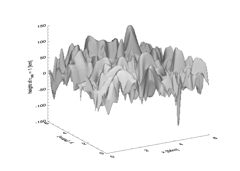
Figure 1: Surface of optical depth unity at 500 nm in snapshot MHD30G.

2.2 Derived one-dimensional models

We derived four different one-dimensional averaged atmospheres from model MHD30G. The first model, 1DZ, is derived by averaging all thermodynamical quantities over horizontal planes. The temperature stratification of this average model is shown in Figure 2 (solid curve), together with the two-dimensional histogram of temperatures in MHD30G. The figure clearly shows the large spread in temperature at any given height, in particular in the range at or below $z=0$. Unfortunately, there is no straightforward way of incorporating the convective motions present in the three-dimensional snapshot realistically into one-dimensional averaged models. In particular, the horizontal velocity field $(v_{x},v_{y})$ cannot be directly represented. Even the average of the vertical velocity $v_{z}$ cannot be included if the resulting model is to be static. Moreover, any vertical velocity would have to be projected into the line of sight for observing directions off disk center. Without including any velocities, however, the spectral lines from the one-dimensional model would be much too narrow, and would not sample similar regions of the atmosphere. In order to achieve a similar amount of broadening in the spectral lines calculated from the one-dimensional model as in the average spectrum of the three-dimensional snapshot, we chose to include the average velocities in the commonly employed form of micro-turbulence with a value of one third of the square root of the sum of the squares of the three velocity components. As it turns out, this choice of micro-turbulence closely matches the photospheric values prescribed in semi-empirical models like the VAL3C model (Vernazza et al., 1981) and its later derivatives.

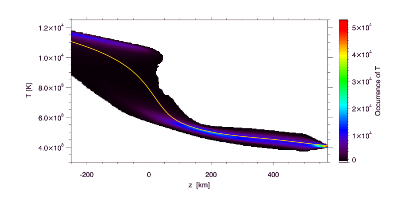
Figure 2: Two-dimensional histogram of temperature values in MHD30G as function of geometric height $z$. The run of the geometrically averaged temperature is plotted with the solid curve.

Since the emergent radiation at a given wavelength typically comes from a narrow range of optical depths around unity, the spatially averaged emergent spectrum from an inhomogeneous atmosphere reflects more the average of atmospheric quantities on an equal optical depth scale than on an equal geometrical height scale. A question to ask is therefore if a one-dimensional atmosphere that is constructed to reproduce an average spectrum can accurately reflect the properties of that atmosphere averaged over equal optical depths. Of course, even if such a one-dimensional representation appears to be successful for the emergent spectrum in the direction and at the wavelength it was constructed for, it is unlikely it will be valid for other directions and wavelengths, since the physical properties sampled by surfaces of equal optical depth in an inhomogeneous atmosphere change with direction and wavelength in a much more complicated way than in a one-dimensional atmosphere. In fact, for more and more inclined viewing angles, a spatially averaged spectrum gradually changes from representing an average over surfaces of equal optical depth to one of averages over equal geometrical height.

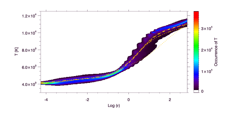
Figure 3: Two-dimensional histogram of temperature in MHD30G as function of optical depth at 500 nm in the vertical direction. Average temperature stratifications of models 1DTAU (dashed), 1DT4 (dot-dashed), and 1DHSE (dot-dot-dot-dashed), and 1DZ (dotted) are plotted against their proper optical depth scale at 500 nm.

To test the premise of how well an equal optical depth averaged model can reproduce the average spectrum of an inhomogeneous atmosphere and its CLV we constructed a one-dimensional model atmosphere from the MHD30G snapshot by computing the opacities at 500 nm in each of its columns and reinterpolating all atmospheric properties to a common optical depth scale at that wavelength (e.g., Kiselman & Nordlund, 1995; Ayres et al., 2006; Koesterke et al., 2008). We average temperature in two different ways, by averaging $T$ and by averaging $T^{4}$ ($\left<T\right>=\left<T^{4}\right>^{1/4}$), as advocated by Steffen et al. (1995) to better preserve radiative flux. We refer to these models as 1DTAU, and 1DT4 hereafter. Steffen et al. (1995) determined that averaging the fourth power of temperature to derive the average temperature provided the best way of reproducing the average spectrum of an inhomogeneous convective model of a white dwarf atmosphere. Figure 3 shows that the differences in stratification between these two prescriptions of averaging temperature are subtle, as also found by Steffen et al. (1995) in their white dwarf modeling, and Steffen & Holweger (2002) in two-dimensional solar convection modeling (their figure 3). A fourth one-dimensional model, named 1DHSE, was constructed by taking model 1DTAU and applying hydrostatic equilibrium, so that the vertical force balance in the model is self consistent. This change of models was accomplished while keeping the relation between temperature and column mass scale fixed, which preserves the total mass in the model, but does not preserve the $T$–$\tau_{500}$ relation of the 1DTAU model. Another option would have been to transition from one model to the other while keeping the optical depth scale at a given wavelength (possibly 500 nm) fixed, but we opted for the former option because it is commonly used in semi-empirical modeling, and would be the solution favored by a hydrodynamic code programmed to find a static solution. The latter option, by the choice of the reference wavelength, introduces even more arbitrariness into the process of defining one-dimensional models than is already the case with the choice of the wavelength at which equal opacity surfaces for averaging are defined.

The obtained average temperature stratifications as a function of the proper optical depth at 500 nm are drawn in Figure 3 over the two-dimensional histogram of temperature values versus optical depth in the three-dimensional snapshot. Note that the slope of the temperature stratification of model 1DZ is much shallower than that of both 1DTAU and 1DT4 and to some degree 1DHSE. The difference arises from the interaction between the temperature and density structure of the granulation, and the nature of the H^- opacity, which scales strongly non-linearly with temperature (proportional to $T^{10}$, see Stein & Nordlund, 1998). Because the H^- opacity increases so strongly with temperature, dense material that resides in the relatively cool intergranular lanes contributes at higher average temperature to the geometrically averaged density. The average opacity of the geometrically averaged atmosphere is therefore much higher than in the optical depth averaged models, at the same temperature. This is visible in the shift towards the right of the dotted curve in Figure 3 with respect to the dashed and dot-dashed curves, and the dot-dot-dot-dashed curve in the higher layers. The difference between the two classes of averaged temperature profiles disappears at smaller optical depths because of the diminished influence of convection in these layers which results in optical depth surfaces that are less corrugated in geometrical height. At much larger depth the topology of the convective flow is dominated by broad, connected, relatively homogeneous upflows, interspersed with narrow isolated downflows, again resulting in a convergence of the $T$—$\tau$ curves, apart from the 1DHSE model. The latter has a shallower gradient in the deeper layers than 1DTAU and 1DT4, because the three-dimensional stratification is in part supported by hydrodynamical forces that are not accounted for in hydrostatic equilibrium, so that the atmosphere has to adjust by increasing pressure and density in the lower layers, which causes its $T$–$\tau$ curve to shift to the right.

2.3 Spectral synthesis

For synthesis of spectra from the different models we used the one- and three-dimensional versions of the transfer code developed by Uitenbroek (1998, 2000, 2001). The different versions of this transfer code share routines that perform common tasks that are independent of geometry, like the solution of chemical equilibrium, calculation of line absorption coefficients, and evaluation of background opacities, which greatly facilitates comparison between results from the different versions. The main difference between the one- and three-dimensional version is the way the formal solution of the transfer equation is obtained. The one-dimensional version uses a Feautrier difference scheme as formulated by Rybicki & Hummer (1991, their appendix A), while the three-dimensional version employs the short-characteristics integral method formulated by Kunasz & Auer (1988) as adapted to periodic boundary conditions by Auer et al. (1994), which is much more numerically efficient in multi-dimensional geometry.

To test for possible differences in emergent intensity that could arise from using two different formal solvers, we created a three-dimensional atmosphere with constant horizontal properties by replicating our geometrically averaged model 1DZ on a $50\times 50$ horizontal grid and calculated the center-to-limb variation of the emergent intensity at 500 and 800 nm in one- and three-dimensional geometry. The resulting intensities, plotted in Figure 4, match very closely, providing confidence that the two formal solvers give very similar results when given the same stratification of source function and opacities, even though they use completely different numerical methods.

Figure 4: Comparison of CLV of emergent intensities from model 1DZ at 500 nm (solid curve) and 800 nm (dashed curve) with the spatially averaged intensities (symbols) from a three-dimensional model constructed by replicating the same stratification on a $50\times 50$ horizontal grid with the same grid spacing as in model MHD30G.

All transfer calculations used in this paper were performed in Local Thermodynamical Equilibrium (LTE), except for the contributions of Thomson scattering by free electrons, Rayleigh scattering by neutral hydrogen and helium atoms, and H₂ molecules, which were lambda iterated. Other background opacity sources that were included were bound–free and free–free transitions of H^- and neutral hydrogen, free–free transitions of H${}_{2}^{-}$, and H${}_{2}^{+}$, and bound–free transitions of different metals. Instantaneous chemical equilibrium was assumed for all molecular concentrations and the non-linear set of chemical equilibrium equations for H₂ and CO was solved iteratively with a Newton-Raphson procedure.

2.3.1 Wavelengths and spectral lines

We compare intensities emergent from our three models in several visible continuum wavelengths, ranging from 400 to 800 nm, one infrared continuum at 4.7 $\mu$m, two Fe I lines at 525.0 and 525.3 nm, respectively, and the 7–6 R69 at 4663.6 nm in the fundamental rotation-vibration band of the CO molecule. The continuum wavelengths were chosen to span a range in formation heights in the solar photosphere corresponding to the maximum of the H^- opacity (near 800 nm) to its minimum (the H^- opacity at 400 nm is very similar to that at 1.6 $\mu$m), in the visible range of the spectrum. In addition, we included the infrared continuum close to the CO line, also because it represents the spectrum at a wavelength where the Planck function varies nearly linearly with temperature.

The two iron lines are very close in wavelength and strength, to eliminate variations resulting from differences in formation height, but have a significant difference in excitation energy of their lower levels. The CO line was included to investigate the effect of the non-linear dependence on temperature of molecular concentrations on line formation. Parameters for the lines are listed in Table 1.

Table 1: Parameters of the spectral lines.

Line	$\log{gf}$	$\chi_{\textrm{exc}}[eV]$
Fe I 525.0209 nm	-4.938	0.121
Fe I 525.3462 nm	-1.670	3.223
CO 7-6 R69 4663.6 nm	-2.585	2.616

2.4 The effect of inhomogeneities on averaging

The horizontal inhomogeneities in temperature and density in the atmosphere not only affect the averaging of opacity but also that of other physical properties that depend on these principal quantities. Since many of these quantities do not scale linearly with temperature and/or density, the operation of averaging the properties of an inhomogeneous atmosphere to a one-dimensional stratification (independent of whether this is done on equal optical depth or geometrical height scales) and evaluating the sought after physical quantity, does not give the same result as evaluating the quantity in the inhomogeneous atmosphere and then averaging it.

2.4.1 Molecular densities

An illustrative example for the effect of inhomogeneities in temperature and density, is the calculation of the number density of a diatomic molecule AB, which in chemical equilibrium, is given by the Saha equation:

$$\frac{n_{A}n_{B}}{n_{AB}}=\left(\frac{2\pi m_{AB}kT}{h^{2}}\right)^{3/2}e^{-D/kT}\left[\frac{U_{A}(T)U_{B}(T)}{Q_{AB}(T)}\right]=\Phi(T),$$ (1)

where $n_{A,B,AB}$ are the number densities for the atomic species A,B and molecule AB, $m_{AB}$ is the reduced mass of the molecule, $k$ and $h$ are the Boltzmann and Planck constants, respectively, $D$ is the dissociation energy and $U_{A,B}$ and $Q_{AB}$ are the atomic and molecular partition functions. Given Equation (1) it is trivial to see that in general

$$\left<\frac{n_{A}n_{B}}{n_{AB}}\right>\neq\Phi(<T>),$$ (2)

when averaging molecular densities in a region with temperature inhomogeneities. In particular, non-linear effects are larger for smaller temperatures. In fact, under the assumptions of low molecular concentrations ($n_{AB}\ll n_{A},n_{B}$) and small temperature perturbations, we can assume that $n_{A}n_{B}$ and the partition functions are approximately constant, so that

$$n_{AB} = C\left(\frac{D}{kT}\right)^{3/2}e^{D/kT}\equiv C\phi(T)$$ (3)

$$C \equiv n_{A}n_{B}\left(\frac{h^{2}}{2\pi m_{AB}D}\right)^{3/2}\left[\frac{Q_{AB}}{U_{A}U_{B}}\right].$$ (4)

Let us now estimate the average molecular density $\left<n_{AB}(T)\right>$ in an inhomogeneous atmosphere with temperature fluctuations $\Delta T$ around $\overline{T}=\left<T\right>$ with $\Delta T/\overline{T}\ll 1$, and compare this average with the concentration $n_{AB}(\overline{T})$ of the molecule at the average temperature. Using a Taylor expansion of Equation 3 in $t=\Delta T/\overline{T}$ around $\overline{T}$ we derive to second order in $t$:

$$\left<\Delta n_{AB}\right>=\frac{1}{2}\left<t^{2}\right>C\left.\frac{\textrm{d}^{2}\phi(t)}{\textrm{d}t^{2}}\right|_{t=0}+\mathcal{O}(\left<t^{3}\right>),$$ (5)

since $\left<\Delta T\right>=0$ by definition. In Appendix A we show that the second derivative of $\phi(t)$ is given by

$$\phi^{\prime\prime}|_{t=0}=\left\{\frac{15}{4}+5\frac{D}{k\overline{T}}+\left(\frac{D}{k\overline{T}}\right)^{2}\right\}n_{AB}(\overline{T}),$$ (6)

which is strictly positive, so that $<n_{AB}>$ is always greater than $n_{AB}(\overline{T})$ when temperature fluctuations are present in the atmosphere.

Note that, for typical temperatures in the solar photosphere of $\overline{T}=5.0\times 10^{3}$ K and the dissociation energy of the CO molecule $D_{CO}=11.091$ eV, the ratio $D_{CO}/k\overline{T}=25.7$, causing the Taylor series used for Equation 5 to converge only if typical fluctuations $\Delta T/\overline{T}$ are smaller than $k\overline{T}/D_{CO}$, or about 4%. In particular for the next term in the expansion to be ignored we should have $\left<(\Delta T/\overline{T})^{3}\right><(k\overline{T}/D_{CO})^{3}$. However, it is straightforward to show that all even-order derivatives are positive, so that the claim that the average abundance of a molecule in an inhomogeneous atmosphere is always larger than the abundance in a homogeneous atmosphere with the same temperature stratification still holds.

Similarly, it can be shown that density inhomogeneities contribute strictly positively to the average molecular number density. In fact, for small molecular concentrations $n_{AB}\ll n_{A},n_{B}$ the number density $n_{AB}$ scales with the square of the hydrogen density (see Equation 1):

$$n_{AB}\propto A_{A}A_{B}\,n_{H}^{2},$$ (7)

where $A_{A,B}$ are the abundances of elements A and B, and $n_{H}$ is the hydrogen number density. This implies that in an inhomogeneous atmosphere with perturbations $\Delta n_{H}$ with $\left<\Delta n_{H}\right>=0$ the average change in molecular number density for molecule AB obeys $\left<\Delta n_{AB}\right>\propto A_{A}A_{B}\left<(\Delta n_{H})^{2}\right>$, which is again strictly positive for non-zero hydrogen number-density inhomogeneities.

Figure 5: CO number densities in snapshot MHD30G averaged over surfaces of equal optical depth at 500 nm (solid curve), and in the one-dimensionalmodels, 1DTAU (dashed curve) 1DT4 (dot-dashed), 1DHSE (dot-dot-dot-dashed) and 1DZ (dotted).

The effects of temperature and density inhomogeneities on the averaging of number densities of the CO molecule is clearly seen in the difference between the curves in Figure 5, which show the average CO number density over surfaces of equal optical depth of CO in the three-dimensional snapshot MHD30G as a function of optical depth (solid curve), and the run of CO densities in the four different one-dimensional models. Even though the average temperature and hydrogen density in MHD30G are the same as the temperature and density in the 1DTAU model at each height, the spatial variation of temperature and density in the three-dimensional model causes the average CO density to be higher at each height in MHD30G than the CO density at the corresponding height in 1DTAU, and the same effect is more or less true in the other averaged models as well. Interestingly, the CO density at the top of the 1DHSE model drops well below the concentrations in the other models. This is the result of enforcing hydrostatic equilibrium. The convective overshoot produces a high density (and pressure, leading to horizontal expansion) over the granular surfaces. In establishing hydrostatic equilibrium, which keeps the column mass – $T$ relation constant, this over pressure causes a vertical extension of the atmosphere, reducing densities at the top. In this reduced density the CO equilibrium shifts towards dissociation.

Since the considered multi-dimensional atmosphere has both temperature and density inhomogeneities, it is hard to estimate what the precise contribution from either is to the differences in average molecular density. We conclude that average one-dimensional models underestimate densities compared to the spatially averaged number density in the inhomogeneous models they are derived from, and therefore result in an overestimate of the required abundances of the constituent atoms of the molecules under consideration. This matches the conclusions by Kiselman & Nordlund (1995) and Scott et al. (2006) who found that oxygen and carbon abundances derived from molecular diagnostics OH and CO lines, respectively, were larger for their average one-dimensional models than from their three-dimensional snapshots.

2.4.2 Comparison between low- and high-excitation line

Figure 6: Number densities $n_{i}$ of the lower level of the low-excitation 525.0 nm and high-excitation 525.3 nm lines in MHD30G (solid curve) and 1DTAU (dashed).

In our line selection we chose two Fe I lines of similar strength and wavelength, but very different excitation potential. Here we investigate if temperature and density inhomogeneities affect their lower level populations, and therefore the line opacities, differently. Indeed, Figure 6 shows that the lower-level populations are affected very differently: those of the 525.0 nm line are enhanced by the inhomogeneities, while those of the 525.3 nm line are diminished by them. The differences in the latter occur below $\tau_{500}=1$, and will likely not affect the intensities in the line. It is also worth to notice that the two lines have similar strength because the large difference in their excitation potentials, which is reflected in the large differences of the populations numbers, is compensated by the difference in their oscillator strength (cf. Table 1).

3 Comparison of spectra

The emission of radiation is a non-linear process with respect to the main physical parameters of the atmosphere. As a consequence, differences must be expected when comparing radiative emission obtained from the five atmospheric models investigated, even when the MHD30G and 1DTAU, for instance, have exactly the same average thermal stratification (in optical depth at 500 nm). As an example, Figure 7 shows the CLV of intensity obtained in four continua, sampling various heights in the atmosphere, namely 400, 500, 800 nm and 4.7 $\mu$m. The first thing to remark is the strong deviation of the intensity of model 1DZ with respect to that in the other models, at all wavelengths except the longest one.This strong deviation of the 1DZ intensities is caused by the shallow temperature-tau relation shown in Figure 3, and is also clearly demonstrated in the results of Trujillo Bueno & Shchukina (2009). It makes obvious that models derived by geometrically averaging atmospheric properties are very far from reality for quantitative spectroscopic analysis, except perhaps for very small $\mu$ values, where the intensity forms in layers where the temperature and density variations are strongly reduced. At the shortest wavelength the averaged intensity from model MHD30G is best approximated by 1DHSE, while the other equal-$\tau$ averaged models underestimate the intensity, in particular at disk center. However, at longer wavelengths the two $\tau$-averaged models perform better. Clearly, none of the four one-dimensional models predicts the CLV of continuum intensity accurately for the whole wavelength range.

Figure 7: CLV of continuum intensities at 400 nm, 500 nm, 800 nm, and 4700 nm for the four one-dimensionalmodels 1DZ (dotted), 1DTAU (dashed), 1DT4 (dot-dashed) and 1DHSE (dot-dot-dot-dashed), and the spatially averaged continua of MHD30G (solid curves).

The differences between the intensities from the MHD30G (solid) and 1DTAU (dashed) and 1DT4 (dot-dashed) models decrease with longer wavelengths, vanishing almost completely at 4.7 $\mu$m, and are mainly the result of the non-linearity of the Planck function as function of temperature. In LTE the emergent intensity is to first order given by the Planck function at optical depth unity at the wavelength under consideration. The surface-averaged intensity, of a three-dimensional atmosphere is therefore given by:

$$\left<I_{\lambda}\right>_{xy}=\left<B_{\lambda}(T)\right>_{\tau_{\lambda}=1}$$ (8)

Let the $\tau_{\lambda}=1$ surface have temperature perturbations $\Delta T$ around an average temperature $\overline{T}$, with $\Delta T/\overline{T}\ll 1$. We want to compare the spatially averaged emergent intensity at wavelength $\lambda$ with the emergent intensity of a one-dimensional atmosphere with temperature stratification equal to the average temperature of the inhomogeneous model on each of its constant optical depth surfaces, i.e. we would like to estimate

$$\left<\Delta B_{\lambda}\right>=\text@frac{1}{2}\left<t^{2}\right>\left.\frac{\textrm{d}^{2}B_{\lambda}(t)}{\textrm{d}t^{2}}\right|_{t=0}+\mathcal{O}(\left<t^{3}\right>),$$ (9)

defining $t\equiv\Delta T/\overline{T}$, as before, and remembering that $\left<t\right>=0$. It is straightforward (if somewhat tedious) to show that the second derivative of the Planck function is strictly positive with a value that strongly decreases with wavelength (see Equation B5). As a consequence the average radiation in the continuum coming from an inhomogeneous atmosphere is always larger than that coming from a homogeneous atmosphere with the same thermal stratification (average temperature–tau relation), consistent with the behavior of the differences between the emergent continuum intensities of models MHD30G and 1DTAU as plotted in Figure 7. To verify the accuracy of Equation 9 we calculated the values for $\overline{T}$, $\left<\Delta T/\overline{T}\right>$, and $\left.B^{\prime\prime}(t)\right|_{t=0}$ on the surface of optical depth unity at 500 nm in model MHD30G, and found that this estimate accounts for 86% of the difference in disk-center intensity with model 1DTAU at that wavelength. The rest of the difference can be ascribed to inaccuracy of the Eddington-Barbier approximation (Appendix B, Equation 8), and neglected higher orders in Equation 9.

Because of the strong increase of the H^- free-free opacity with wavelength, the continuum in the infrared at 4.7 $\mu$m forms in higher atmospheric layers, where the temperature difference between the models vanishes. Moreover, at this long wavelength the Planck function varies linearly with temperature (its second derivative vanishes), thus reducing the effect of temperature inhomogeneities discussed above. Both together cause the near equality of the 4.7 $\mu$m continuum curves in Figure 7.

We thus confirm and explain the difference in CLV of continuum intensities between one- and three-dimensional atmospheres with the same temperature stratification as described by Koesterke et al. (2008), though a direct comparison is difficult since these authors compare their results as a difference to observed CLV, and normalize to disk-center intensities. If we would interpret the observed CLV of intensity in the continuum, in particular at shorter wavelengths, in terms of a one-dimensional atmosphere, we would overestimate the average temperature gradient of the atmosphere (as measured on surfaces of constant optical depth), since temperature inhomogeneities raise the average emergent intensity at disk center, steepening the CLV.

Model 1DHSE is clearly too hot in the higher layers (see Figure 3), giving rise to an overestimate of intensities, in particular at longer wavelengths, which form relatively higher in the atmosphere.

Figure 8: Average line profiles for the MHD30G (solid curves), and 1DTAU (dashed) and 1DZ (dotted), 1DT4 (dot-dashed) and 1DHSE (dot-dot-dot-dashed) models, for the viewing angles coresponding to $\mu=0.3,0.5$ and $1.0$.

Calculated profiles of the Fe I 525.0 and 525.3 nm line and CO 7-6 R69 line for three different viewing angles are shown in Figure 8. As expected, the profiles from the one-dimensional models lack the asymmetries produced by MHD30G. In addition, we note that differences in intensity of the line-cores are smaller than in nearby continua, because the former originate higher in the atmosphere, where amplitudes of temperature inhomogeneities are reduced (Figures 2 and 3). However, the averaged line-core intensity in the MHD30G model is systematically higher because of these remaining inhomogeneities, while the core intensities of the two one-dimensional models are virtually indistinguishable because they have the same temperature in the core-forming part of the models, apart from model 1DHSE, which is too hot in this region.

To estimate the effect the spatial averaging in the different models has on the determination of element abundances we have matched the equivalent widths in each of the one-dimensional models and lines with the one from the average spectrum of model MHD30G by varying the abundances of iron and oxygen, respectively. The resulting differences are expressed in dex and tabulated in Table 2, with negative values meaning that the one-dimensional models would require a downward revision of the abundance (and thus that their use would lead to an underestimate of the abundance). Typical abundance differences are small but significant, in agreement with the findings of Steffen & Holweger (2002), who tabulate abundance determination differences between their two-dimensional convection simulation and similarly derived one-dimensional averaged models.

Table 2: Differences with abundance derived by matching the equivalent width of disk-center line profiles with that in MHD30G.

$\lambda$ (nm)	525.0	525.3	4663
1DZ	+0.06	+0.09	-0.02
1DTAU	-0.09	-0.09	-0.07
HSE	+0.03	-0.02	-0.15
T4	-0.07	-0.09	-0.03

We note that these determined abundance differences should in no way be considered abundance corrections, as we have made no effort to properly adjust microturbulence, and our estimates are based on the equivalent width of disk center intensity rather than that of the disk-integrated flux. Instead the numbers in Table 2 are an indication of the typical error that can be made by using different models. Clearly, the abundance correction that would be implied by our CO line analysis is opposite of what we would expect from the CO number density that we presented in Section 2.4.1. The bottom panel in Figure 8 makes evident what the reason for this discrepancy is. In particular, the 1DHSE model has a significantly increased continuum level, which increases the concomitant equivalent width, requiring a negative abundance correction, rather than a positive. The temperature stratification of the 1DHSE model here plays a larger role than the reduced CO concentration in that stratification.

The CO line from MHD30G broaden its wings towards the limb (bottom panel of Figure 8) because of the effect of horizontal convective motions on the relatively narrow line, which has reduced thermal broadening due to the weight of the CO molecule. This broadening would contribute significantly to the equivalent width of the disk-integrated flux profile, and would change the abundance correction we give in table 2 a more positive value, if we were to use the equivalent width of the flux profile rather than that of the disk-center intensity. It is clear, therefore, that different line formation effects can play opposite roles in the abundance determination. These effects are very hard to keep track of in the gross simplifications that are performed when representing a three-dimensional structured atmosphere with a one-dimensional averaged model, no matter how sophisticated the latter is constructed.

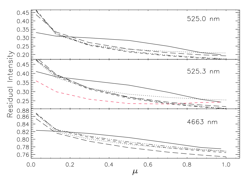
Figure 9: CLVs of the residual line core intensity of the Fe I 525.0, 525.3 nm and 4663.6 nm CO lines in the five models MHD30G (solid curves), 1DTAU (dashed), 1DZ (dotted), 1DT4 (dot-dashed) and 1DHSE (dot-dot-dot-dashed). Red dashed curve shows the average resudual line core intensity behavior in the three-dimensional model when horizontal velocities are set to zero.

Differences between line spectra in the one- and three-dimensional models are even more evident in the CLV of the residual line-core intensities (defined as $(I_{\textrm{cont}}-I_{\textrm{core}})/I_{\textrm{cont}}$) plotted in Figure 9. Strikingly, the residual line-core intensities of the two iron lines in model MHD30G show a much shallower decrease with decreasing $\mu$ than the core intensities in the averaged models. Given the imposed equality of the average thermal stratifications of models 1DTAU and MHD30G, the stark difference between their line-core CLVs must be the result of mass motions that are properly taken into account in the three-dimensional model, but represented by microturbulence in the one-dimensional derivatives. Indeed, by eliminating the horizontal and vertical velocities, respectively, we determined that the CLV behavior of the line cores is the result of the presence of horizontal motions in the convective model. Setting these to zero results in a CLV that behaves similarly as function of $\mu$ as in the one-dimensionalmodels (red dashed line in Figure 9 in the midle panel).

The CLV behavior of the average residual line-core intensity in the MHD30G model can be explained in the following way. For moderate viewing angles the horizontal convective velocities shift the core opacity out of the center of the line, lowering the formation height at those wavelengths, sampling higher temperatures, broadening the line and increasing the line core intensity. By contrast, the vertical velocities result in the familiar convective blue-shift because of the combined effect of the area asymmetries of down- and up-flows and the correlation between brightness and up-flows. Clearly, the line-core CLV will affect disk-integrated line intensities, and other derived line parameters, which are used in stellar abundance determinations.

4 Discussion and conclusion

The analysis of stellar spectra would greatly benefit if it would be possible to extract many physical parameters accurately through one-dimensional modeling. The radiative transfer in this type of models is orders of magnitude less computationally demanding than in self consistent and more realistic three-dimensional (M)HD models. In this paper we have attempted to further clarify if such a less numerically demanding approach is feasible, and if not, what the physical reasons for failure could be. We have approached this question in the simplest possible fashion by comparing spectra in several continua and lines from one-dimensional atmospheres that were derived from a three-dimensional MHD snapshot by straight averaging over equal geometric heights and over surfaces of equal optical depth at 500 nm. In this way we assured as much as possible that the derived one-dimensional atmospheres had the same average properties as the original snapshot, so that possible differences between the spectra are mostly the result of the inhomogeneities in the three-dimensional model. As a result we have identified several mechanisms that affect the average spectrum of the inhomogeneous three-dimensional model that cannot be adequately represented in derived one-dimensional models, and thus would lead to wrong estimates of the physical parameters extracted from the spectrum, if that spectrum were to be interpreted in the context of simpler one-dimensional models.

In particular, we constructed two types of one-dimensional spatially averaged atmospheric stratifications, 1DZ, and 1DTAU and 1DT4, respectively, by averaging the thermodynamic properties of a single snapshot, MHD30G, from simulation of solar magneto-convection, over surfaces of equal geometric height and equal optical depth at 500 nm. In addition, we created a model, 1DHSE, by taking model 1DTAU and allowing its stratification to be determined by hydrostatic equilibrium. We then calculated the intensities in continua at 400, 500, 800 nm, and 4.7 $\mu$m, two Fe I lines at 525.0 and 525.3 nm, and a CO molecular line at 4663 nm from all five models, compared the spatially averaged spectra from the three-dimensional model at different viewing angles with those from the average-property one-dimensional models at the same angles.

From the calculated spectra it is immediately clear that the geometrically averaged model 1DZ provides a particularly poor representation of the average properties of the three-dimensional model in terms of spectroscopic diagnostics. The geometric averaging results in a temperature–$\tau$ stratification that is much shallower than the stratification of average temperature in the inhomogeneous atmosphere, and thus results in much lower continuum intensities at disk center, and a much shallower CLV. Only very close to the limb where intensities emanate from relatively higher layers of the atmosphere that are less affected by granulation and thus more homogeneous, and where the obliquity of the rays naturally averages over horizontal inhomogeneities, the intensities from this model converge on the averaged ones from MHD30G.

It is no surprise that intensities derived from models 1DTAU and 1DT4 are much closer to the spatially averaged ones from model MHD30G, as radiation at a given wavelength naturally comes from a layer with limited range in optical depth around unity. Yet, even in continua the average intensity from model MHD30G lies well above those of the tau-averaged models, in particular at shorter wavelengths, and closer to disk center. This underestimate of continuum intensities by the one-dimensional models is the result of the non-linear mapping of temperature inhomogeneities into intensity fluctuations by the Planck function. In Section 3 we show that the average intensity of an atmosphere with temperature fluctuations is always higher than the intensity of a homogeneous atmosphere with the same average temperature stratification, because of the strict positivity of the second derivative of the Planck function with temperature. For large temperature and/or long wavelengths the second derivative of $B_{\lambda}$ vanishes, and temperature inhomogeneities are mapped linearly into intensity variations, so that differences between the three-dimensional and derived one-dimensional models disappear, as is evident in the continuum at 4.7 $\mu$m (Figure 7). A corollary of the non-linear mapping of the Planck function is that the interpretation of an average spectrum from a horizontally inhomogeneous atmosphere, in terms of a one-dimensional model will lead to an overestimate of the average temperature gradient in the atmosphere.

Molecular lines are often used in abundance determinations, because they are generally weak, less affected by thermal broadening because of their mass, and plentiful. However, their concentration is sensitive to thermal conditions. To investigate how temperature and density inhomogeneities affect the average concentration molecules and emergent spectra of their lines, we calculated the CO number densities in the inhomogeneous model MHD30D and averaged models 1DTAU and 1DZ, as well as the emergent spectrum of the CO 7-6 R68 rotation-vibration line for different viewing angles. In Section 2.4.1 we show that the presence of both temperature and density inhomogeneities to first order always lead to an increase of the average molecular density of a diatomic molecule over the values in a homogeneous atmosphere with the same average temperature and density stratification. As an example we show the calculated number density of the CO molecule in models MHD30G and 1DTAU as a function of average optical depth in Figure 5. The underestimate of molecular densities by a one-dimensional model that is used to represent the average of an inhomogeneous atmosphere will lead to an overestimate of the abundances of the constituent atoms of the molecule if molecular lines are used for determination of these abundances.

It is obvious that one-dimensional average-property models cannot represent the complex mass motions that result from convection. One effect that the average models necessarily fail to incorporate is the convective blue shift and line characteristic “C-shaped” asymmetry of the bisectors of spectral lines that results from the correlation of brightness and upflows and asymmetry between up- and downflows in the convective flows. We identify one other important aspect of the convective flows that one-dimensional models lack, namely the broadening and line weakening that horizontal motions produce for moderate viewing angles ($\mu\approx 0.7$). The weakening results from the shift of opacity out of the line core by horizontal motions, both to the red and to the blue, increasing formation height and raising the central intensity. This effect leads to an initial increase in the line-core intensity as function of increasing viewing angle (decreasing $\mu$), and a much shallower decline of the residual line-core intensity as is clearly shown in Figure 9. The horizontal velocity effect is apertly absent in the CLVs obtained from the one-dimensional models. It thus also affects the disk-integrated line profile shape that will therefore be wrongly interpreted if analyzed in the context of such average-property models. Observational evidence for the the shallow behavior of the residual line-core intensity is seen in Rodriguez Hidalgo et al. (1994) who determined the CLV of this property in the Fe I 593.02 nm line, among others. Curiously, the Mn I 539.47 nm line shows behavior more in line with our results from the one-dimensional models. This is perhaps the result of the large hyperfine structure broadening of manganese lines, which makes them less susceptible to convective velocity broadening, as explained by Vitas et al. (2009).

In summary, our comparison of spectra, and analysis of the physical effects of temperature and density inhomogeneities make clear that extreme caution has to be taken when the average spectrum of a horizontally inhomogeneous atmosphere is interpreted in the context of a one-dimensional atmospheric representation. Not only the lack of incorporation of convective motions into one-dimensional models, but also the non-linearities involved in establishing molecular equilibrium and level populations as function of temperature and density, and the non-linearities of the Planck function as function of temperature likely lead to misinterpretation of the observed spectrum. In the work here we have concentrated on spatial averaging, but our derivations and contentions hold equally well in case of temporal averaging. In addition, we suspect that non-linearities introduced by non-LTE conditions, which we have not addressed in this paper, have to be treated with even more caution. The realism of chromospheric modeling, which still relies heavily on one-dimensional models, therefore needs careful examination in this respect. A very illustrative example is given by the simulations presented by Carlsson & Stein (1994), who simulate acoustic shock propagation in the solar atmosphere. The shocks heat the atmosphere, but their main effect is an enhancement of chromospheric emission. When the resulting time-averaged spectrum is modeled with a one-dimensional hydrostatic semi-empirical model, the resulting atmosphere is required to have a chromospheric temperature rise. This temperature rise is very much at odds with the mean temperature stratification of the simulations which shows a monotonic decline with height.

Since the 1DTAU model we employed exactly matches the average thermal stratification of the three-dimensional snapshot, but produces different intensity values in lines, and even continua, we conclude that a one-dimensional model that reproduces the average spectrum of an inhomogeneous atmosphere necessarily has a different average stratification than this atmosphere. It is therefore in our opinion not possible to produce a one-dimensional atmospheric model that is at the same time spectroscopically equivalent and has matching average physical properties.

Appendix A Second derivative of $\phi$

The function $\phi(T)$ is defined (Equation 3) as:

$$\phi(T)\equiv\left(\frac{D}{kT}\right)^{3/2}\exp{\left[\frac{D}{kT}\right]}.$$ (A1)

Writing $T=\overline{T}+\Delta T$ and defining $t\equiv\Delta T/\overline{T}$ we can write $\phi$ as a function of $t$:

$$\phi(t)=\left(\frac{D}{k\overline{T}}\right)^{3/2}\frac{1}{(1+t)^{3/2}}\exp{\left[\frac{D}{k\overline{T}}\left(\frac{1}{1+t}\right)\right]}.$$ (A2)

It follows that the first derivative of this function with respect to $t$ is

$$\phi^{\prime}(t)=-\left\{\frac{3}{2}\frac{1}{(1+t)}+\frac{D}{k\overline{T}}\frac{1}{(1+t)^{2}}\right\}\phi(t),$$ (A3)

and its second derivative

$$\phi^{\prime\prime}(t)=\left\{\frac{15}{4}\frac{1}{(1+t)^{2}}+5\frac{D}{k\overline{T}}\frac{1}{(1+t)^{3}}+\left(\frac{D}{k\overline{T}}\right)^{2}\frac{1}{(1+t)^{4}}\right\}\phi(t).$$ (A4)

Appendix B Second derivative of the Planck function

The Planck function for wavelength $\lambda$ and temperature $T$ is given by:

$$B_{\lambda}(T)=\frac{2hc^{2}}{\lambda^{5}}\frac{1}{e^{\frac{hc}{\lambda kT}}-1}$$ (B1)

Writing $T=\overline{T}+\Delta T$, and defining $t\equiv\Delta T/\overline{T}$ and $b\equiv hc/\lambda k\overline{T}$, we rewrite $B$ as a function of $t$:

$$B_{\lambda}(t)=\frac{2hc^{2}}{\lambda^{5}}\frac{1}{e^{\frac{b}{1+t}}-1}$$ (B2)

It follows that

$$B^{\prime}_{\lambda}(t)=\frac{b}{(1+t)^{2}}\frac{1}{1-e^{\frac{-b}{1+t}}}B_{\lambda}(t),$$ (B3)

and

$$B^{\prime\prime}_{\lambda}(t)=\frac{b}{1-e^{\frac{-b}{1+t}}}\frac{1}{(1+t)^{3}}\left\{\left(\frac{1+e^{\frac{-b}{1+t}}}{1-e^{\frac{-b}{1+t}}}\right)\frac{b}{1+t}\right\}B_{\lambda}(t).$$ (B4)

For $t=0$ the second derivative is

$$\left.B^{\prime\prime}_{\lambda}(t)\right|_{t=0}=\frac{b}{1-e^{-b}}\left\{\left(\frac{1+e^{-b}}{1-e^{-b}}\right)b-2\right\}\left.B_{\lambda}(t)\right|_{t=0}.$$ (B5)

The expression between curly brackets in Equation B5 is strictly positive for all $b$, and vanishes for $b<<1$, i.e., for large wavelength, large temperature, or both.

References

- Abbett (2007) Abbett, W. P. 2007, ApJ, 665, 1469
- Allende Prieto et al. (2001) Allende Prieto, C., Lambert, D. L., & Asplund, M. 2001, ApJ, 556, L63
- Allende Prieto et al. (2002) Allende Prieto, C., Lambert, D. L., & Asplund, M. 2002, ApJ, 573, L137
- Asplund (2005) Asplund, M. 2005, ARA&A, 43, 481
- Asplund et al. (2005) Asplund, M., Grevesse, N., Sauval, A. J., Allende Prieto, C., & Blomme, R. 2005, A&A, 431, 693
- Asplund et al. (2004) Asplund, M., Grevesse, N., Sauval, A. J., Allende Prieto, C., & Kiselman, D. 2004, A&A, 417, 751
- Asplund et al. (2000a) Asplund, M., Nordlund, Å., Trampedach, R., Allende Prieto, C., & Stein, R. F. 2000a, A&A, 359, 729
- Asplund et al. (2000b) Asplund, M., Nordlund, Å., Trampedach, R., & Stein, R. F. 2000b, A&A, 359, 743
- Atroshchenko & Gadun (1994) Atroshchenko, I. N., & Gadun, A. S. 1994, A&A, 291, 635
- Auer et al. (1994) Auer, L., Fabiani Bendicho, P., & Trujillo Bueno, J. 1994, A&A, 292, 599
- Avrett & Loeser (2008) Avrett, E. H., & Loeser, R. 2008, ApJS, 175, 229
- Ayres et al. (2006) Ayres, T. R., Plymate, C., & Keller, C. U. 2006, ApJS, 165, 618
- Caffau et al. (2010) Caffau, E., Ludwig, H., Bonifacio, P., Faraggiana, R., Steffen, M., Freytag, B., Kamp, I., & Ayres, T. R. 2010, A&A, 514, A92
- Carlsson & Stein (1994) Carlsson, M., & Stein, R. F. 1994, in M. Carlsson (ed.), Proceeding of the Oslo mini-workshop on Chromospheric Dynamics, Institute for Theoretical Astrophysics, Oslo, Norway, p. 25
- Centeno et al. (2008) Centeno, R., Trujillo Bueno, J., Uitenbroek, H., & Collados, M. 2008, ApJ, 677, 742
- Ermolli et al. (2010) Ermolli, I., Criscuoli, S., Uitenbroek, H., Giorgi, F., Rast, M. P., & Solanki, S. K. 2010, A&A, 523, A55+
- Fontenla et al. (2009) Fontenla, J. M., Curdt, W., Haberreiter, M., Harder, J., & Tian, H. 2009, ApJ, 707, 482
- Freytag et al. (2002) Freytag, B., Steffen, M., & Dorch, B. 2002, Astronomische Nachrichten, 323, 213
- Grigoryeva et al. (2009) Grigoryeva, S. A., Teplitskaya, R. B., & Ozhogina, O. A. 2009, Astronomy Reports, 53, 569
- Hayek et al. (2010) Hayek, W., Asplund, M., Carlsson, M., Trampedach, R., Collet, R., Gudiksen, B. V., Hansteen, V. H., & Leenaarts, J. 2010, A&A, 517, A49
- Holweger et al. (1990) Holweger, H., Heise, C., & Kock, M. 1990, A&A, 232, 510
- Holweger & Müller (1974) Holweger, H., & Müller, E. A. 1974, Sol. Phys., 39, 19
- Jacoutot et al. (2008) Jacoutot, L., Kosovichev, A. G., Wray, A., & Mansour, N. N. 2008, ApJ, 684, L51
- Kiselman & Nordlund (1995) Kiselman, D., & Nordlund, A. 1995, A&A, 302, 578
- Koesterke et al. (2008) Koesterke, L., Allende Prieto, C., & Lambert, D. L. 2008, ApJ, 680, 764
- Kunasz & Auer (1988) Kunasz, P. B., & Auer, L. H. 1988, J. Quant. Spec. Radiat. Transf., 39, 67
- Muthsam et al. (2010) Muthsam, H. J., Kupka, F., Löw-Baselli, B., Obertscheider, C., Langer, M., & Lenz, P. 2010, New Astronomy, 15, 460
- Nordlund & Stein (2001) Nordlund, Å., & Stein, R. F. 2001, ApJ, 546, 576
- Pereira et al. (2009) Pereira, T. M. D., Asplund, M., & Kiselman, D. 2009, A&A, 508, 1403
- Ramírez et al. (2009) Ramírez, I., Allende Prieto, C., Koesterke, L., Lambert, D. L., & Asplund, M. 2009, A&A, 501, 1087
- Rodriguez Hidalgo et al. (1994) Rodriguez Hidalgo, I., Collados, M., & Vazquez, M. 1994, A&A, 283, 263
- Rybicki & Hummer (1991) Rybicki, G. B., & Hummer, D. G. 1991, A&A, 245, 171
- Schaffenberger et al. (2005) Schaffenberger, W., Wedemeyer-Böhm, S., Steiner, O., & Freytag, B. 2005, in D. E. Innes, A. Lagg, & S. A. Solanki (ed.), Chromospheric and Coronal Magnetic Fields, Vol. 596 of ESA Special Publication
- Scott et al. (2006) Scott, P. C., Asplund, M., Grevesse, N., & Sauval, A. J. 2006, A&A, 456, 675
- Serenelli et al. (2009) Serenelli, A. M., Basu, S., Ferguson, J. W., & Asplund, M. 2009, ApJ, 705, L123
- Shapiro et al. (2010) Shapiro, A. I., Schmutz, W., Schoell, M., Haberreiter, M., & Rozanov, E. 2010, A&A, 517, A48+
- Shchukina et al. (2005) Shchukina, N. G., Trujillo Bueno, J., & Asplund, M. 2005, ApJ, 618, 939
- Socas-Navarro (2007) Socas-Navarro, H. 2007, ApJS, 169, 439
- Socas-Navarro & Uitenbroek (2004) Socas-Navarro, H., & Uitenbroek, H. 2004, ApJ, 603, L129
- Steffen & Holweger (2002) Steffen, M., & Holweger, H. 2002, A&A, 387, 258
- Steffen et al. (1995) Steffen, M., Ludwig, H., & Freytag, B. 1995, A&A, 300, 473
- Stein & Nordlund (1989) Stein, R. F., & Nordlund, Å. 1989, ApJ, 342, L95
- Stein & Nordlund (1998) Stein, R. F., & Nordlund, Å. 1998, ApJ, 499, 914
- Stein & Nordlund (2000) Stein, R. F., & Nordlund, Å. 2000, Sol. Phys., 192, 91
- Stein & Nordlund (2001) Stein, R. F., & Nordlund, Å. 2001, ApJ, 546, 585
- Stein et al. (2009) Stein, R. F., Nordlund, Å., & Asplund, M. 2009, Living Reviews in Solar Physics, 6(2)
- Trujillo Bueno & Shchukina (2009) Trujillo Bueno, J., & Shchukina, N. 2009, ApJ, 694, 1364
- Uitenbroek (1998) Uitenbroek, H. 1998, ApJ, 498, 427
- Uitenbroek (2000) Uitenbroek, H. 2000, ApJ, 531, 571
- Uitenbroek (2001) Uitenbroek, H. 2001, ApJ, 557, 389
- Vernazza et al. (1981) Vernazza, J. E., Avrett, E. H., & Loeser, R. 1981, ApJS, 45, 635
- Vitas et al. (2009) Vitas, N., Viticchiè, B., Rutten, R. J., & Vögler, A. 2009, A&A, 499, 301
- Vögler et al. (2005) Vögler, A., Shelyag, S., Schüssler, M., Cattaneo, F., Emonet, T., & Linde, T. 2005, A&A, 429, 335
- Wilson & Williams (1972) Wilson, P. R., & Williams, N. V. 1972, Sol. Phys., 26, 30