A Novel Probabilistic Pruning Approach to Speed Up Similarity Queries in Uncertain Databases

Abstract

In this paper, we propose a novel, effective and efficient probabilistic pruning criterion for probabilistic similarity queries on uncertain data. Our approach supports a general uncertainty model using continuous probabilistic density functions to describe the (possibly correlated) uncertain attributes of objects. In a nutshell, the problem to be solved is to compute the PDF of the random variable denoted by the probabilistic domination count: Given an uncertain database object $B$, an uncertain reference object $R$ and a set $\mathcal{D}$ of uncertain database objects in a multi-dimensional space, the probabilistic domination count denotes the number of uncertain objects in $\mathcal{D}$ that are closer to $R$ than $B$. This domination count can be used to answer a wide range of probabilistic similarity queries. Specifically, we propose a novel geometric pruning filter and introduce an iterative filter-refinement strategy for conservatively and progressively estimating the probabilistic domination count in an efficient way while keeping correctness according to the possible world semantics. In an experimental evaluation, we show that our proposed technique allows to acquire tight probability bounds for the probabilistic domination count quickly, even for large uncertain databases.

I Introduction

In the past two decades, there has been a great deal of interest in developing efficient and effective methods for similarity queries, e.g. $k$-nearest neighbor search, reverse $k$-nearest neighbor search and ranking in spatial, temporal, multimedia and sensor databases. Many applications dealing with such data have to cope with uncertain or imprecise data.

In this work, we introduce a novel scalable pruning approach to identify candidates for a class of probabilistic similarity queries. Generally spoken, probabilistic similarity queries compute for each database object $o\in\mathcal{D}$ the probability that a given query predicate is fulfilled. Our approach addresses probabilistic similarity queries where the query predicate is based on object (distance) relations, i.e. the event that an object $B$ belongs to the result set depends on the relation of its distance to the query object $R$ and the distance of another object $A$ to the query object. Exemplarily, we apply our novel pruning method to the most prominent queries of the above mentioned class, including the probabilistic $k$-nearest neighbor (P$k$NN) query, the probabilistic reverse $k$-nearest neighbor (PR$k$NN) query and the probabilistic inverse ranking query.

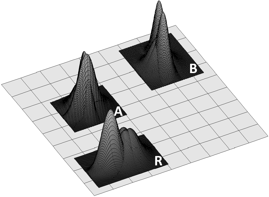
Figure 1: $A$ dominates $B$ w.r.t. $R$ with high probability.

I-A Uncertainty Model

In this paper, we assume that the database $\mathcal{D}$ consists of multi-attribute objects $o_{1},...,o_{N}$ that may have uncertain attribute values. An uncertain attribute is defined as follows:

Definition 1 (Probabilistic Attribute).

A probabilistic attribute $attr$ of object $o_{i}$ is a random variable drawn from a probability distribution with density function $f^{attr}_{i}$.

An uncertain object $o_{i}$ has at least one uncertain attribute value. The function $f_{i}$ denotes the multi-dimensional probability density distribution (PDF) of $o_{i}$ that combines all density functions for all probabilistic attributes $attr$ of $o_{i}$.

Following the convention of uncertain databases [6, 8, 9, 11, 14, 21, 24], we assume that $f_{i}$ is (minimally) bounded by an uncertainty region $R^{i}$ such that $\forall x\notin R^{i}:f_{i}(x)=0$ and

$$\int_{R^{i}}f_{i}(x)dx\leq 1.$$

Specifically, the case $\int_{R^{i}}f_{i}(x)dx<1$ implements existential uncertainty, i.e. object $o_{i}$ may not exist in the database at all with a probability greater than zero. In this paper we focus on the case $\int_{R^{i}}f_{i}(x)dx=1$, but the proposed concepts can be easily adapted to existentially uncertain objects. Although our approach is also applicable for unbounded PDF, e.g., Gaussian PDF, here we assume $f_{i}$ exceeds zero only within a bounded region. This is a realistic assumption because the spectrum of possible values of attributes is usually bounded and it is commonly used in related work, e.g. [8, 9] and [6]. Even if $f_{i}$ is given as an unbounded PDF, a common strategy is to truncate PDF tails with negligible probabilities and normalize the resulting PDF. In specific, [6] shows that for a reasonable low truncation threshold, the impact on the accuracy of probabilistic ranking queries is quite low while having a very high impact on the query performance. In this way, each uncertain object can be considered as a $d$-dimensional rectangle with an associated multi-dimensional object PDF (c.f. Figure 1). Here, we assume that uncertain attributes may be mutually dependent. Therefore the object PDF can have any arbitrary form, and in general, cannot simply be derived from the marginal distribution of the uncertain attributes. Note that in many applications, a discrete uncertainty model is appropriate, meaning that the probability distribution of an uncertain object is given by a finite number of alternatives assigned with probabilities. This can be seen as a special case of our model.

I-B Problem Formulation

We address the problem of detecting for a given uncertain object $B$ the number of uncertain objects of an uncertain database $\mathcal{D}$ that are closer to (i.e. dominate) a reference object $R$ than $B$. We call this number the domination count of $B$ w.r.t. $R$ as defined below:

Definition 2 (Domination).

Consider an uncertain database $\mathcal{D}=\{o_{1},...,o_{N}\}$ and an uncertain reference object $R$. Let $A,B\in\mathcal{D}$. $Dom(A,B,R)$ is the random indicator variable that is $1$, iff $A$ dominates $B$ w.r.t. $R$, formally:

$$Dom(A,B,R)=\begin{cases}1,&\text{if }dist(a,r)<dist(b,r)\\ &\forall a\in A,b\in B,r\in R\\ 0,&\text{otherwise}\end{cases}$$

where $a,b$ and $r$ are samples drawn from the PDFs of $A,B$ and $R$, respectively and $dist$ is a distance function on vector objects.

Definition 3 (Domination Count).

Consider an uncertain database $\mathcal{D}=\{o_{1},...,o_{N}\}$ and an uncertain reference object $R$. For each uncertain object $B\in\mathcal{D}$, let $DomCount(B,R)$ be the random variable of the number of uncertain objects $A\in\mathcal{D}$ ($A\neq B$) that are closer to $R$ than $B$:

$$DomCount(B,R)=\sum_{A\in\mathcal{D},A\neq B}Dom(A,B,R)$$

$DomCount(B,R)$ is the sum of $N-1$ non-necessarily identically distributed and non-necessarily independent Bernoulli variables. The problem solved in this paper is to efficiently compute the probability density distribution of $DomCount(B,R)(B\in\mathcal{D})$ formally introduced by means of the probabilistic domination (cf. Section III) and the probabilistic domination count (cf. Section IV).

Determining domination is a central module for most types of similarity queries in order to identify true hits and true drops (pruning). In the context of probabilistic similarity queries, knowledge about the PDF of $DomCount(B,R)$ can be used to find out if $B$ satisfies the query predicate. For example, for a probabilistic 5NN query with probability threshold $\tau=10\%$ and query object $Q$, an object $B$ can be pruned (returned as a true hit), if the probability $P(DomCount(B,Q)<5)$ is less (more) than $10\%$.

I-C Overview

Given an uncertain database $\mathcal{D}=\{o_{1},...,o_{N}\}$ and an uncertain reference object $R$, our objective is to efficiently derive the distribution of $DomCount(B,R)$ for any uncertain object $B\in\mathcal{D}$ and use it in the computation of probabilistic similarity queries. First (Section III), we build on the methodology of [15] to efficiently find the complete set of objects in $\mathcal{D}$ that definitely dominate (are dominated by) $B$ w.r.t. $R$. At the same time, we find the set of objects whose dominance relationship to $B$ is uncertain. Using a decomposition technique, for each object $A$ in this set, we can derive a lower and an upper bound for $PDom(A,B,R)$, i.e., the probability that $A$ dominates $B$ w.r.t. $R$. In Section IV, we show that due to dependencies between object distances to $R$, these probabilities cannot be combined in a straightforward manner to approximate the distribution of $DomCount(B,R)$. We propose a solution that copes with these dependencies and introduce techniques that help to to compute the probabilistic domination count in an efficient way. In particular, we prove that the bounds of $PDom(A,B,R)$ are mutually independent if they are computed without a decomposition of $B$ and $R$. Then, we provide a class of uncertain generating functions that use these bounds to build the distribution of $DomCount(B,R)$. We then propose an algorithm which progressively refines $DomCount(B,R)$ by iteratively decomposing the objects that influence its computation (Section V). Section VI shows how to apply this iterative probabilistic domination count refinement process to evaluate several types of probabilistic similarity queries. In Section VII, we experimentally demonstrate the effectiveness and efficiency of our probabilistic pruning methods for various parameter settings on artificial and real-world datasets.

II Related Work

The management of uncertain data has gained increasing interest in diverse application fields, e.g. sensor monitoring [12], traffic analysis, location-based services [27] etc. Thus, modelling probabilistic databases has become very important in the literature, e.g. [1, 23, 24]. In general, these models can be classified in two types: discrete and continuous uncertainty models. Discrete models represent each uncertain object by a discrete set of alternative values, each associated with a probability. This model is in general adopted for probabilistic databases, where tuples are associated with existential probabilities, e.g. [14, 19, 25, 16].

In this work, we concentrate on the continuous model in which an uncertain object is represented by a probability density function (PDF) within the vector space. In general, similarity search methods based on this model involve expensive integrations of the PDFs, hence special approximation and indexing techniques for efficient query processing are typically employed [13, 26].

Uncertain similarity query processing has focused on various aspects. A lot of existing work dealing with uncertain data addresses probabilistic nearest neighbor (NN) queries for certain query objects [11, 18] and for uncertain queries [17]. To reduce computational effort, [9] add threshold constraints in order to retrieve only objects whose probability of being the nearest neighbor exceeds a user-specified threshold to control the desired confidence required in a query answer. Similar semantics of queries in probabilistic databases are provided by Top-$k$ nearest neighbor queries [6], where the $k$ most probable results of being the nearest neighbor to a certain query point are returned. Existing solutions on probabilistic $k$-nearest neighbor ($k$NN) queries restrict to expected distances of the uncertain objects to the query object [22] or also use a threshold constraint [10]. However, the use of expected distances does not adhere to the possible world semantics and may thus produce very inaccurate results, that may have a very small probability of being an actual result ([25, 19]). Several approaches return the full result to queries as a ranking of probabilistic objects according to their distance to a certain query point [4, 14, 19, 25]. However, all these prior works have in common that the query is given as a single (certain) point. To the best of our knowledge, $k$-nearest neighbor queries as well as ranking queries on uncertain data, where the query object is allowed to be uncertain, have not been addressed so far. Probabilistic reverse nearest neighbor (RNN) queries have been addressed in [7] to process them on data based on discrete and continuous uncertainty models. Similar to our solution, the uncertainty regions of the data are modelled by MBRs. Based on these approximations, the authors of [7] are able to apply a combination of spatial, metric and probabilistic pruning criteria to efficiently answer queries.

All of the above approaches that use MBRs as approximations for uncertain objects utilize the minimum/maximum distance approximations in order to remove possible candidates. However, the pruning power can be improved using geometry-based pruning techniques as shown in [15]. In this context, [20] introduces a geometric pruning technique that can be utilized to answer monochromatic and bichromatic probabilistic RNN queries for arbitrary object distributions.

The framework that we introduce in this paper can be used to answer probabilistic (threshold) $k$NN queries and probabilistic reverse (threshold) $k$NN queries as well as probabilistic ranking and inverse ranking queries for uncertain query objects.

III Similarity Domination on Uncertain Data

In this section, we tackle the following problem: Given three uncertain objects $A$, $B$ and $R$ in a multidimensional space $\mathbb{R}^{d}$, determine whether object $A$ is closer to $R$ than $B$ w.r.t. a distance function defined on the objects in $\mathbb{R}^{d}$. If this is the case, we say $A$ dominates $B$ w.r.t. $R$. In contrast to [15], where this problem is solved for certain data, in the context of uncertain objects this domination relation is not a predicate that is either true or false, but rather a (dichotomous) random variable as defined in Definition 2. In the example depicted in Figure 1, there are three uncertain objects $A$, $B$ and $R$, each bounded by a rectangle representing the possible locations of the object in $\mathbb{R}^{2}$. The PDFs of $A$, $B$ and $R$ are depicted as well. In this scenario, we cannot determine for sure whether object $A$ dominates $B$ w.r.t. $R$. However, it is possible to determine that object $A$ dominates object $B$ w.r.t. $R$ with a high probability. The problem at issue is to determine the probabilistic domination probability defined as:

Definition 4 (Probabilistic Domination).

Given three uncertain objects $A$, $B$ and $R$, the probabilistic domination $PDom(A,B,R)$ denotes the probability that $A$ dominates $B$ w.r.t. $R$.

Naively, we can compute $PDom(A,B,R)$ by simply integrating the probability of all possible worlds in which $A$ dominates $B$ w.r.t. $R$ exploiting inter-object independency:

$$PDom(A,B,R)=\int_{a\in A}\int_{b\in B}\int_{r\in R}\delta(a,b,r)\cdot P(A=a)\cdot P(B=b)\cdot P(R=r)da\,db\,dr,$$

where $\delta(a,b,r)$ is the following indicator function:

$$\delta(a,b,r)=\begin{cases}1,&\text{if }dist(a,r)<dist(b,r)\\ 0,&\text{else}\end{cases}$$

The problem of this naive approach is the computational cost of the triple-integral. The integrals of the PDFs of A, B and R may in general not be representable as a closed-form expression and the integral of $\delta(a,b,r)$ does not have a closed-from expression. Therefore, an expensive numeric approximation is required for this approach. In the rest of this section we propose methods that efficiently derive bounds for $PDom(A,B,R)$, which can be used to prune objects avoiding integral computations.

III-A Complete Domination

First, we show how to detect whether $A$ completely dominates $B$ w.r.t. $R$ (i.e. if $PDom(A,B,R)=1$) regardless of the probability distributions assigned to the rectangular uncertainty regions. The state-of-the-art criterion to detect spatial domination on rectangular uncertainty regions is with the use of minimum/maximum distance approximations. This criterion states that $A$ dominates $B$ w.r.t. $R$ if the minimum distance between $R$ and $B$ is greater than the maximum distance between $R$ and $A$. Although correct, this criterion is not tight (cf. [15]), i.e. not each case where $A$ dominates $B$ w.r.t. $R$ is detected by the min/max-domination criterion. The problem is that the dependency between the two distances between $A$ and $R$ and between $B$ and $R$ is ignored. Obviously, the distance between $A$ and $R$ as well as the distance between $B$ and $R$ depend on the location of $R$. However, since $R$ can only have a unique location within its uncertainty region, both distances are mutually dependent. Therefore, we adopt the spatial domination concepts proposed in [15] for rectangular uncertainty regions.

Corollary 1 (Complete Domination).

Let $A,B,R$ be uncertain objects with rectangular uncertainty regions. Then the following statement holds:

$$PDom(A,B,R)=1\Leftrightarrow\sum_{i=1}^{d}\max\limits_{r_{i}\in\{R_{i}^{min},R_{i}^{max}\}}(\textit{MaxDist}(A_{i},r_{i})^{p}-\textit{MinDist}(B_{i},r_{i})^{p})<0,$$

where $A_{i},B_{i}$ and $R_{i}$ denote the projection interval of the respective rectangular uncertainty region of $A$, $B$ and $R$ on the $i^{th}$ dimension; $R_{i}^{min}$ $(R_{i}^{max})$ denotes the lower (upper) bound of interval $R_{i}$, and $p$ corresponds to the used $L_{p}$ norm. The functions $\textit{MaxDist}(A,r)$ and $\textit{MinDist}(A,r)$ denote the maximal (respectively minimal) distance between the one-dimensional interval $A$ and the one-dimensional point $r$.

Corollary 1 follows directly from [15]; the inequality is true if and only if for all points $a\in A,b\in B,r\in R$, $a$ is closer to $r$ than $b$. Translated into the possible worlds model, this is equivalent to the statement that $A$ is closer to $R$ than $B$ for any possible world, which in return means that $PDom(A,B,R)=1$.

In addition, it holds that

Corollary 2.

$$PDom(A,B,R)=1\Leftrightarrow PDom(B,A,R)=0$$

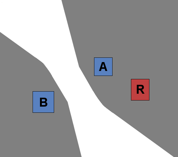
(a) Complete domination

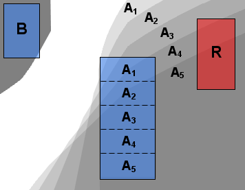
(b) Probabilistic domination

Figure 2: Similarity Domination.

In the example depicted in Figure 2(a), the grey region on the right shows all points that definitely are closer to $A$ than to $B$ and the grey region on the left shows all points that definitely are closer to $B$ than to $A$. Consequently, $A$ dominates $B$ ($B$ dominates $A$) if $R$ completely falls into the right (left) grey shaded half-space.

III-B Probabilistic Domination

Now, we consider the case where $A$ does not completely dominate $B$ w.r.t. $R$. In consideration of the possible world semantics, there may exist worlds in which $A$ dominates $B$ w.r.t. $R$, but not all possible worlds satisfy this criterion. Let us consider the example shown in Figure 2(b) where the uncertainty region of $A$ is decomposed into five partitions, each assigned to one of the five grey-shaded regions illustrating which points are closer to the partition in $A$ than to $B$. As we can see, $R$ only completely falls into three grey-shaded regions. This means that $A$ does not completely dominate $B$ w.r.t. $R$. However, we know that in some possible worlds (at least in all possible words where $A$ is located in $A_{1}$, $A_{2}$ or $A_{3}$) $A$ does dominate $B$ w.r.t. $R$. The question at issue is how to determine the probability $PDom(A,B,R)$ that $A$ dominates $B$ w.r.t. $R$ in an efficient way. The key idea is to decompose the uncertainty region of an object $X$ into subregions for which we know the probability that $X$ is located in that subregion (as done for object $A$ in our example). Therefore, if neither $Dom(A,B,R)$ nor $Dom(B,A,R)$ holds, then there may still exist subregions $A^{\prime}\subset A$, $B^{\prime}\subset B$ and $R^{\prime}\subset R$ such that $A^{\prime}$ dominates $B^{\prime}$ w.r.t. $R^{\prime}$. Given disjunctive decomposition schemes $\mathcal{\underline{A}}$, $\mathcal{\underline{B}}$ and $\mathcal{\underline{R}}$ we can identify triples of subregions ($A^{\prime}\in\mathcal{\underline{A}}$, $B^{\prime}\in\mathcal{\underline{B}}$, $R^{\prime}\in\mathcal{\underline{R}}$) for which $Dom(A^{\prime},B^{\prime},R^{\prime})$ holds. Let $\delta(A^{\prime},B^{\prime},R^{\prime})$ be the following indicator function:

$$\delta(A^{\prime},B^{\prime},R^{\prime})=\begin{cases}1,&\text{if }Dom(A^{\prime},B^{\prime},R^{\prime})\\ 0,&\text{else}\end{cases}$$

Lemma 1.

Let $A,B$ and $R$ be uncertain objects with disjunctive object decompositions $\mathcal{\underline{A}},\mathcal{\underline{B}}$ and $\mathcal{\underline{R}}$, respectively. To derive a lower bound $PDom_{LB}(A,B,R)$ of the probability $PDom(A,B,R)$ that $A$ dominates $B$ w.r.t. $R$, we can accumulate the probabilities of combinations of these subregions as follows:

$$PDom_{LB}(A,B,R)=\sum_{A^{\prime}\in\mathcal{\underline{A}},B^{\prime}\in\mathcal{\underline{B}},R^{\prime}\in\mathcal{\underline{R}}}P(a\in A^{\prime})\cdot P(b\in B^{\prime})\cdot P(r\in R^{\prime})\cdot\delta(A^{\prime},B^{\prime},R^{\prime}),$$

where $P(X\in X^{\prime})$ denotes the probability that object $X$ is located within the region $X^{\prime}$.

Proof.

The probability of a combination $(A^{\prime},B^{\prime},R^{\prime})$ can be computed by $P(a\in A^{\prime})\cdot P(b\in B^{\prime})\cdot P(r\in R^{\prime})$ due to the assumption of mutually independent objects. These probabilities can be aggregated due to the assumption of disjunctive subregions, which implies that any two different combinations of subregions $(A^{\prime}\in\mathcal{\underline{A}},B^{\prime}\in\mathcal{\underline{B}},R^{\prime}\in\mathcal{\underline{R}})$ and $(A^{\prime\prime}\in\mathcal{\underline{A}},B^{\prime\prime}\in\mathcal{\underline{B}},R^{\prime\prime}\in\mathcal{\underline{R}}$, $A^{\prime}\neq A^{\prime\prime}\vee B^{\prime}\neq B^{\prime\prime}\vee R^{\prime}\neq R^{\prime\prime}$ must represent disjunctive sets of possible worlds. It is obvious that all possible worlds defined by combinations $(A^{\prime},B^{\prime},R^{\prime})$ where $\delta(A^{\prime},B^{\prime},R^{\prime})=1$, $A$ dominates $B$ w.r.t. $R$. But not all possible worlds where $A$ dominates $B$ w.r.t. $R$ are covered by these combinations and, thus, do not contribute to $PDom_{LB}(A,B,R)$. Consequently, $PDom_{LB}(A,B,R)$ lower bounds $PDom(A,B,R)$. ∎

Analogously, we can define an upper bound of $PDom(A,B,R)$:

Lemma 2.

An upper bound $PDom_{UB}(A,B,R)$ of $PDom(A,B,R)$ can be derived as follows:

$$PDom_{UB}(A,B,R)=1-PDom_{LB}(B,A,R)$$

Naturally, the more refined the decompositions are, the tighter the bounds that can be computed and the higher the corresponding cost of deriving them. In particular, starting from the entire MBRs of the objects, we can progressively partition them to iteratively derive tighter bounds for their dependency relationships until a desired degree of certainty is achieved (based on some threshold). However, in the next section, we show that the derivation of the domination count $DomCount(B,R)$ of a given object $B$ (cf. Definition 3), which is the main module of prominent probabilistic queries cannot be straightforwardly derived with the use of these bounds and we propose a methodology based on generating functions for this purpose.

IV Probabilistic Domination Count

In Section III we described how to conservatively and progressively approximate the probability that $A$ dominates $B$ w.r.t. $R$. Given these approximations $PDom_{LB}(A,B,R)$ and $PDom_{UB}(A,B,R)$, the next problem is to cumulate these probabilities to get an approximation of the domination count $DomCount(B,R)$ of an object $B$ w.r.t. $R$ (cf. Definition 3). To give an intuition how challenging this problem is, we first present a naive solution that can yield incorrect results due to ignoring dependencies between domination relations in Section IV-A. To avoid the problem of dependent domination relations, we first show in Section IV-B how to exploit object independencies to derive domination bounds that are mutually independent. Afterwards, in Section IV-C, we introduce a new class of uncertain generating functions that can be used to derive bounds for the domination count efficiently, as we show in Section IV-D. Finally, in Section IV-E, we show how to improve our domination count approximation by considering disjunct subsets of possible worlds for which a more accurate approximation can be computed.

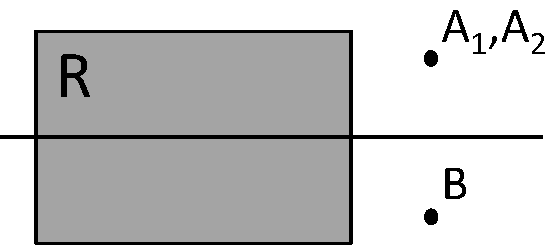
Figure 3: $A_{1}$ and $A_{2}$ dominate $B$ w.r.t. $R$ with a probability of 50%, respectively.

IV-A The Problem of Domination Dependencies

To compute $DomCount(B,R)$, a straightforward solution is to first approximate $PDom(A,B,R)$ for all $A\in\mathcal{D}$ using the technique proposed in Section III. Then, given these probabilities we can apply the technique of uncertain generating functions (cf. Section IV-C) to approximate the probability that exactly $0$, exactly $1$, …, exactly $n-1$ uncertain objects dominate $B$. However, this approach ignores possible dependencies between domination relationships. Although we assume independence between objects, the random variables $Dom(A_{1},B,R)$ and $Dom(A_{2},B,R)$ are mutually dependent because the distance between $A_{1}$ and $R$ depends on the distance between $A_{2}$ and $R$ because object $R$ can only appear once. Consider the following example:

Example 1.

Consider a database of three certain objects $B$, $A_{1}$ and $A_{2}$ and the uncertain reference object $R$, as shown in Figure 3. For simplicity, objects $A_{1}$ and $A_{2}$ have the same position in this example. The task is to determine the domination count of $B$ w.r.t. $R$. The domination half-space for $A_{1}$ and $A_{2}$ is depicted here as well. Let us assume that $A_{1}$ ($A_{2}$) dominates $B$ with a probability of $PDom(A_{1},B,R)=PDom(A_{2},B,R)=50\%$. Recall that this probability can be computed by integration or approximated with arbitrary precision using the technique of Section III. However, in this example, the probability that both $A_{1}$ and $A_{2}$ dominate $B$ is not simply $50\%\cdot 50\%=25\%$, as the generating function technique would return.

The reason for the wrong result in this example, is that the generating function requires mutually independent random variables. However, in this example, it holds that if and only if $R$ falls into the domination half-space of $A_{1}$, it also falls into the domination half-space of $A_{2}$. Thus we have the dependency $dom(A_{1},B,R)\leftrightarrow dom(A_{2},B,R)$ and the probability for $R$ to be dominated by both $A_{1}$ and $A_{2}$ is

$$P(dom(A_{1},B,R))\cdot P(dom(A_{2},B,R)|dom(A_{1},B,R))=0.5\cdot 1=0.5.$$

IV-B Domination Approximations Based on Independent Objects

In general, domination relations may have arbitrary correlations. Therefore, we present a way to compute the domination count $DomCount(B,R)$ while accounting for the dependencies between domination relations.

Complete Domination

In an initial step, complete domination serves as a filter which allows us to detect those objects $A\in\mathcal{D}$ that definitely dominate a specific object $B$ w.r.t. $R$ and those objects that definitely do not dominate $B$ w.r.t. $R$ by means of evaluating $PDom(A,B,R)$. It is important to note that complete domination relations are mutually independent, since complete domination is evaluated on the entire uncertainty regions of the objects. After applying complete domination, we have detected objects that dominate $B$ in all, or no possible worlds. Consequently, we get a first approximation of the domination count $DomCount(B,R)$, obviously, it must be higher than the number $N$ of objects that dominate $B$ and lower than $|\mathcal{D}|-M$, where $M$ is the number of objects that dominate $B$ in no possible world, i.e. $P(DomCount(B,R)=k)=0$ for $k\leq N$ and $k\geq|\mathcal{D}|-M$. Nevertheless, for $N<k<|\mathcal{D}-M|$ we still have a very bad approximation of the domination count probability of $0\leq P(DomCount(B,R)=k)\leq 1$.

Probabilistic Domination

In order to refine this probability distribution, we have to take the set of influence objects $influenceObjects=\{A_{1},...,A_{C}\}$, which neither completely prune $B$ nor are completely dominated by $B$ w.r.t. $R$. For each $A_{i}\in influenceObjects$, $0<PDom(A_{i},B,R)<1$. For these objects, we can compute probabilities $PDom(A_{1},B,R),...,PDom(A_{C},B,R)$ according to the methodology in Section III. However, due to the mutual dependencies between domination relations (cf. Section IV-A), we cannot simply use these probabilities directly, as they may produce incorrect results. However, we can use the observation that the objects $A_{i}$ are mutually independent and each candidate object $A_{i}$ only appears in a single domination relation $Dom(A_{1},B,R),...,Dom(A_{C},B,R)$. Exploiting this observation, we can decompose the objects $A_{1},...,A_{C}$ only, to obtain mutually independent bounds for the probabilities $PDom(A_{1},B,R),...,PDom(A_{C},B,R)$, as stated by the following lemma:

Lemma 3.

Let $A_{1},...A_{C}$ be uncertain objects with disjunctive object decompositions $\mathcal{A}_{1},...,\mathcal{A}_{C}$, respectively. Also, let $B$ and $R$ be uncertain objects (without any decomposition). The lower (upper) bound $PDom_{LB}(A_{i},B,R)$ ($PDom_{UB}(A_{i},B,R)$) as defined in Lemma 1 (Lemma 2) of the random variable $Dom(A_{i},B,R)$ is independent of the random variable $Dom(A_{j},B,R)$ ($1\leq i\neq j\leq C$).

Proof.

Consider the random variable $Dom(A_{i},B,R)$ conditioned on the event $Dom(A_{j},B,R)=1$. Using Equation 1, we can derive the lower bound probability of $Dom(A_{i},B,R)=1|Dom(A_{j},B,R)=1$ as follows:

$$PDom_{LB}(A_{i},B,R|Dom(A_{j},B,R)=1)=$$

$$\sum_{A_{i}^{\prime}\in\mathcal{A}_{i},B^{\prime}\in\mathcal{B},R^{\prime}\in\mathcal{R}}[P(a_{i}\in A_{i}^{\prime}|Dom(A_{j},B,R)=1)\cdot P(b\in B^{\prime}|Dom(A_{j},B,R)=1)\cdot$$

$$P(r\in R^{\prime}|Dom(A_{j},B,R)=1)\cdot\delta(A_{i}^{\prime},B^{\prime},R^{\prime})]$$

Now we exploit that $B$ and $R$ are not decomposed, thus $B^{\prime}=B$ and $R^{\prime}=R$, and thus $P(B\in B^{\prime}|Dom(A_{j},B,R)=1)=1=P(B\in B^{\prime})$ and $P(R\in R^{\prime}|Dom(A_{j},B,R)=1)=1=P(R\in R^{\prime})$. We obtain:

$$PDom_{LB}(A_{i},B,R|Dom(A_{j},B,R)=1)=$$

$$\sum_{A_{i}^{\prime}\in\mathcal{A}_{i},B^{\prime}\in\mathcal{B},R^{\prime}\in\mathcal{R}}[P(a_{i}\in A_{i}^{\prime}|Dom(A_{j},B,R)=1)\cdot P(b\in B^{\prime})\cdot P(r\in R^{\prime})\cdot\delta(A_{i}^{\prime},B^{\prime},R^{\prime})]$$

Next we exploit that $P(a_{i}\in A_{i}^{\prime}|Dom(A_{j},B,R)=1)=P(a_{i}\in A_{i}^{\prime})$ since $A_{i}$ is independent from $Dom(A_{j},B,R)$ and obtain:

$$PDom_{LB}(A_{i},B,R|Dom(A_{j},B,R)=1)=$$

$$\sum_{A_{i}^{\prime}\in\mathcal{A}_{i},B^{\prime}\in\mathcal{B},R^{\prime}\in\mathcal{R}}[P(a_{i}\in A_{i}^{\prime})\cdot P(b\in B^{\prime})\cdot P(r\in R^{\prime})\cdot\delta(A_{i}^{\prime},B^{\prime},R^{\prime})]=PDom_{LB}(A_{i},B,R)$$

Analogously, it can be shown that

$$PDom_{UB}(A_{i},B,R|Dom(A_{j},B,R)=1)=PDom_{UB}(A_{i},B,R).$$

∎

In summary, we can now derive, for each object $A_{i}$ a lower and an upper bound of the probability that $A_{i}$ dominates $B$ w.r.t. $R$. However, these bounds may still be rather loose, since we only consider the full uncertainty region of $B$ and $R$ so far, without any decomposition. In Section IV-E, we will show how to obtain more accurate, still mutual independent probability bounds based on decompositions of $B$ and $R$. Due to the mutual independency of the lower and upper probability bounds, these probabilities can now be used to get an approximation of the domination count of $B$. In order to do this efficiently, we adapt the generating functions technique which is proposed in [19]. The main challenge here is to extend the generating function technique in order to cope with probability bounds instead of concrete probability values. It can be shown that a straightforward solution based on the existing generating functions technique applied to the lower/upper probability bounds in an appropriate way does solve the given problem efficiently, but overestimates the domination count probability and thus, does not yield good probability bounds. Rather, we have to redesign the generating functions technique such that lower/upper probability bounds can be handled correctly.

IV-C Uncertain Generating Functions (UGFs)

In this subsection, we will give a brief survey on the existing generating function technique (for more details refer to [19]) and then propose our new technique of uncertain generating functions.

Generating Functions

Consider a set of $N$ mutually independent, but not necessarily identically distributed Bernoulli $\{0,1\}$ random variables $X_{1},...,X_{N}$. Let $P(X_{i})$ denote the probability that $X_{i}=1$. The problem is to efficiently compute the sum

$$\sum_{i=1}^{N}X_{i}=\sum_{i=1}^{N}Dom(A_{i},B,R)$$

of these random variables. A naive solution would be to count, for each $0\leq k\leq N$, all combinations with exactly $k$ occurrences of $X_{i}=1$ and accumulate the respective probabilities of these combinations. This approach, however, shows a complexity of $O(2^{N})$. In [5], an approach was proposed that achieves an $O(N)$ complexity using the Poisson Binomial Recurrence. Note that $O(N)$ time is asymptotically optimal in general, since the computation involves at least $O(N)$ computations, namely $P(X_{i}),1\leq i\leq N$. In the following, we propose a different approach that, albeit having the same linear asymptotical complexity, has other advantages, as we will see. We apply the concept of generating functions as proposed in the context of probabilistic ranking in [19]. Consider the function ${\cal{F}}(x)=\prod^{n}_{i=1}(a_{i}+b_{i}x)$. The coefficient of $x^{k}$ in ${\cal{F}}(x)$ is given by: $\sum_{|\beta|=k}\prod_{i:\beta_{i}=0}a_{i}\prod_{i:\beta_{i}=1}b_{i}$, where $\beta=\langle\beta_{1},...,\beta_{N}\rangle$ is a Boolean vector, and $|\beta|$ denotes the number of 1’s in $\beta$.

Now consider the following generating function:

$${\cal{F}}^{i}=\prod_{X_{i}}(1-P(X_{i})+P(X_{i})\cdot x)=\sum_{j\geq 0}c_{j}x^{j}.$$

The coefficient $c_{j}$ of $x^{j}$ in the expansion of ${\cal{F}}^{i}$ is the probability that for exactly $j$ random variables $X_{i}$ it holds that $X_{i}=1$. Since ${\cal{F}}^{i}$ contains at most $i+1$ non-zero terms and by observing that

$${\cal{F}}^{i}={\cal{F}}^{i-1}\cdot(1-P(X_{i})+P(X_{i})\cdot x),$$

we note that ${\cal{F}}^{i}$ can be computed in $O(i)$ time given ${\cal{F}}^{i-1}$. Since ${\cal{F}}^{0}=1x^{0}=1$, we conclude that ${\cal{F}}^{N}$ can be computed in $O(N^{2})$ time. If only the first $k$ coefficients are required (i.e. coefficients $c_{j}$ where $j<k$), this cost can be reduced to $O(k\cdot N)$, by simply dropping the summands $c_{j}x^{j}$ where $j\geq k$.

Example 2.

As an example, consider three independent random variables $X_{1}$, $X_{2}$ and $X_{3}$. Let $P(X_{1})=0.2$, $P(X_{2})=0.1$ and $P(X_{3})=0.3$, and let $k=2$. Then:

$${\cal{F}}^{1}={\cal{F}}^{0}\cdot(0.8+0.2x)=0.2x^{1}+0.8x^{0}$$

$${\cal{F}}^{2}={\cal{F}}^{1}\cdot(0.9+0.1x)=0.02x^{2}+0.26x^{1}+0.72x^{0}\stackrel{{\scriptstyle*}}{{=}}0.26x^{1}+0.72x^{0}$$

$${\cal{F}}^{3}={\cal{F}}^{2}\cdot(0.7+0.3x)=0.078x^{2}+0.418x^{1}+0.504x^{0}$$

$$\stackrel{{\scriptstyle*}}{{=}}0.418x^{1}+0.504x^{0}$$

Thus, $P(DomCount(B)=0)=50.4\%$ and $P(DomCount(B)=1)=41.8\%$. We obtain $P(DomCount(B)<2)=92.2\%$. Thus, $B$ can be reported as a true hit if $\tau$ is not greater than $92.2\%$. Equations marked by * exploit that we only need to compute the $c_{j}$ where $j<k=2$.

Uncertain Generating Functions

Given a set of $N$ independent but not necessarily identically distributed Bernoulli $\{0,1\}$ random variables $X_{i},1\leq i\leq N$. Let $P_{LB}(X_{i})$ ($P_{UB}(X_{i})$) be a lower (upper) bound approximation of the probability $P(X_{i}=1)$. Consider the random variable

$$\sum_{i=1}^{N}X_{i}.$$

We make the following observation: The lower and upper bound probabilities $P_{LB}(X_{i})$ and $P_{UB}(X_{i})$ correspond to the probabilities of the three following events:

• $X_{i}=1$ definitely holds with a probability of at least $P_{LB}(Dom(A_{i},B,R))$.

• $X_{i}=0$ definitely holds with a probability of at least $1-P_{UB}(X_{i})$.

• It is unknown whether $X_{i}=0$ or $X_{i}=1$ with the remaining probability of $P_{UB}(Dom(A_{i},B,R))-P_{LB}(Dom(A_{i},B,R))=PDom_{UB}(A_{i},B,R)-PDom_{LB}(A_{i},B,R)$.

Based on this observation, we consider the following uncertain generating function (UGF):

$${\cal{F}}^{N}=\prod_{i\in 1,...,N}[(P_{LB}(X_{i})\cdot x+(1-P_{UB}(X_{i}))\cdot y+(P_{UB}(X_{i})-P_{LB}(X_{i})))]=\sum_{i,j\geq 0}c_{i,j}x^{i}y^{j}.$$

The coefficient $c_{i,j}$ has the following meaning: With a probability of $c_{i,j}$, $B$ is definitely dominated at least $i$ times, and possibly dominated another $0$ to $j$ times. Therefore, the minimum probability that $\sum_{i=1}^{N}X_{i}=k$ is $c_{k,0}$, since that is the probability that exactly $k$ random variables $X_{i}$ are $1$. The maximum probability that $\sum_{i=1}^{N}X_{i}=k$ is $\sum_{i\leq k,i+j\geq k}c_{i,j}$, i.e. the total probability of all possible combinations in which $\sum_{i=1}^{N}X_{i}=k$, may hold. Therefore, we obtain an approximated PDF of $\sum_{i=1}^{N}X_{i}$. In the approximated PDF of $\sum_{i=1}^{N}X_{i}$, each probability $\sum_{i=1}^{N}X_{i}=k$ is given by a conservative and a progressive approximation.

Example 3.

Let $P_{LB}(X_{1})=20\%$, $P_{UB}(X_{1})=70\%$, $P_{LB}(X_{2})=60\%$ and $P_{UB}(X_{2})=80\%$. The generating function for the random variable $\sum_{i=1}^{2}X_{i}$ is the following:

$${\cal{F}}^{2}=(0.2x+0.5y+0.3)(0.6x+0.2y+0.2)=0.12x^{2}+0.34x+0.1+0.22xy+0.16y+0.06y^{2}$$

That implies that, with a probability of at least $12\%$, $\sum_{i=1}^{2}X_{i}=2$. In addition, with a probability of $22\%$ plus $6\%$, it may hold that $\sum_{i=1}^{2}X_{i}=2$, so that we obtain a probability bound of $12\%-40\%$ for the random event $\sum_{i=1}^{2}X_{i}=2$. Analogously, $\sum_{i=1}^{2}X_{i}=1$ with a probability of $34\%-78\%$ and $\sum_{i=1}^{2}X_{i}=0$ with a probability of $10\%-32\%$. The approximated PDF of $\sum_{i=1}^{2}X_{i}$ is depicted in Figure 4.

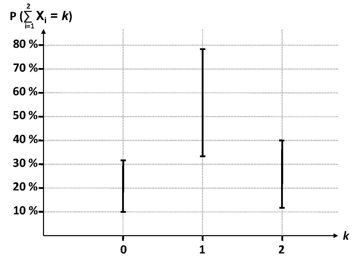
Figure 4: Approximated PDF of $\sum_{i=1}^{2}X_{i}$.

Each expansion ${\cal{F}}^{l}$ can be obtained from the expansion of ${\cal{F}}^{l-1}$ as follows:

$${\cal{F}}^{l}={\cal{F}}^{l-1}\cdot$$

$$[P_{LB}(X_{l})\cdot x+(1-P_{UB}(X_{l}))+(P_{UB}(X_{l})-P_{LB}(X_{l}))\cdot y].$$

We note that ${\cal{F}}^{l}$ contains at most $\sum_{i=1}^{l+1}i$ non-zero terms (one $c_{i,j}$ for each combination of $i$ and $j$ where $i+j\leq l$). Therefore, the total complexity to compute ${\cal{F}}^{l}$ is $O(l^{3})$.

IV-D Efficient Domination Count Approximation using UGFs

We can directly use the uncertain generating functions proposed in the previous section to derive bounds for the probability distribution of the domination count $DomCount(B,R)$. Again, let $\mathcal{D}=A_{1},...,A_{N}$ be an uncertain object database and $B$ and $R$ be uncertain objects in $\mathbb{R}^{d}$. Let $Dom(A_{i},B,R),1\leq i\leq N$ denote the random Bernoulli event that $A_{i}$ dominates $B$ w.r.t. $R$. Also recall that the domination count is defined as the random variable that is the sum of the domination indicator variables of all uncertain objects in the database (cf. Definition 3).

Considering the generating function

$${\cal{F}}^{N}=\prod_{i\in 1,...,N}[(P_{LB}(Dom(A_{i},B,R))\cdot x+(P_{UB}(Dom(A_{i},B,R))-P_{LB}(Dom(A_{i},B,R)))\cdot y)+$$

$$(1-P_{UB}(Dom(A_{i},B,R)))]=\sum_{i,j\geq 0}c_{i,j}x^{i}y^{j},$$ (1)

we can efficiently compute lower and upper bounds of the probability that $DomCount(B,R)=k$ for $0\leq k\leq|\mathcal{D}|$, as discussed in Section IV-C and because the independence property of random variables required by the generating functions is satisfied due to Lemma 3.

Lemma 4.

A lower bound $DomCount_{LB}^{k}(B,R)$ of the probability that $DomCount(B,R)=k$ is given by

$$DomCount_{LB}^{k}(B,R)=c_{k,0}$$

and an upper bound $DomCount_{UB}^{k}(B,R)$ of the probability that $DomCount(B,R)=k$ is given by

$$DomCount_{UB}^{k}(B,R)=\sum_{i\leq k,i+j\geq k}c_{i,j}$$

Example 4.

Assume a database containing uncertain objects $A_{1}$, $A_{2}$, $B$ and $R$. The task is to determine a lower (upper) bound of the domination count probability $DomCount_{LB}^{k}(B,R)$ ($DomCount_{UB}^{k}(B,R)$) of $B$ w.r.t. $R$. Assume that, by decomposing $A_{1}$ and $A_{2}$ and using the probabilistic domination approximation technique proposed in Section III-B, we determine that $A_{1}$ has a minimum probability $PDom_{LB}(A_{1},B,R)$ of dominating $B$ of $20\%$ and a maximum probability $PDom_{UB}(A_{1},B,R)$ of $50\%$. For $A_{2}$, $PDom_{LB}(A_{2},B,R)$ is $60\%$ and $PDom_{UB}(A_{2},B,R)$ is $80\%$. By applying the technique in the previous subsection, we get the same generating function as in Example 3 and thus, the same approximated PDF for the $DomCount(B,R)$ depicted in Figure 4.

To compute the uncertain generating function and thus the probabilistic domination count of an object in an uncertain database of size $N$, the total complexity is $O(N^{3})$. The reason is that the maximal number of coefficients of the generating function ${\cal{F}}^{x}$ is quadratic in $x$, since ${\cal{F}}^{x}$ contains coefficients $c_{i,j}$ where $i+j\leq x$, that is at most $\frac{x^{2}}{2}$ coefficients. Since we have to compute ${\cal{F}}^{x}$ for each ($x<N$), the total time complexity is $O(N^{3})$. Note that only candidate objects $c\in Cand$ for which a complete domination cannot be detected (cf. Section III-A) have to be considered in the generating functions. Thus, the total runtime to compute $DomCount_{LB}^{k}(B,R)$ as well as $DomCount_{UB}^{k}(B,R)$ is $O(|Cand|^{3})$. In addition, we will show in Section VI how to reduce, specifically for $k$NN and R$k$NN queries, the total time complexity to $O(k^{2}\cdot|Cand|)$.

Discussion

In the extended version of this paper ([3]), we show that instead of applying the uncertain generating function to approximate the domination count of $B$, two regular generating functions can be used; one generating function that uses the progressive (lower) bounds $P_{UB}(Dom(A_{i},B,R))$ and one that uses the conservative (upper) probability bounds $P_{UB}(Dom(A_{i},B,R))$. However, we give an intuition and a formal proof that using regular generating functions yields looser bounds for the approximated domination.

IV-E Efficient Domination Count Approximation Based on Disjunctive Worlds

Since the uncertain objects $B$ and $R$ appear in each domination relation $PDom(A_{1},B,R)$,$...$,$PDom(A_{C},B,R)$ that is to evaluate, we cannot split objects $B$ and $R$ independently (cf. Section IV-A). The reason for this dependency is that knowledge about the predicate $Dom(A_{i},B,R)$ may impose constraints on the position of $B$ and $R$. Thus, for a partition $B_{1}\subset B$, the probability $PDom(A_{j},B_{1},R)$ may change given $Dom(A_{i},B,R)$ ($1\leq i,j\leq C,i\neq j$). However, note:

Lemma 5.

Given fixed partitions $B^{\prime}\subseteq B$ and $R^{\prime}\subseteq R$, then the random variables $Dom(A_{i},B^{\prime},R^{\prime})$ are mutually independent for $1\leq i,j\leq C,i\neq j$.

Proof.

Similar to the proof of Lemma 3. ∎

This allows us to individually consider the subset of possible worlds where $b\in B^{\prime}$ and $r\in R^{\prime}$ and use Lemma 5 to efficiently compute the approximated domination count probabilities $DomCount_{LB}^{k}(B^{\prime},R^{\prime})$ and $DomCount_{UB}^{k}(B^{\prime},R^{\prime})$ under the condition that $B$ falls into a partition $B^{\prime}\subseteq B$ and $R$ falls into a partition $R^{\prime}\subseteq R$. This can be performed for each pair $(B^{\prime},R^{\prime})\in\underline{\mathcal{B}}\times\underline{\mathcal{R}}$, where $\underline{\mathcal{B}}$ and $\underline{\mathcal{R}}$ denote the decompositions of $B$ and $R$, respectively. Now, we can treat pairs of partitions $(B^{\prime},R^{\prime})\in\underline{\mathcal{B}}\times\underline{\mathcal{R}}$ independently, since all pairs of partition represent disjunctive sets of possible worlds due to the assumption of a disjunctive partitioning. Exploiting this independency, the PDF of the domination count $DomCount(B,R)$ of the total objects $B$ and $R$ can then be obtained by creating an uncertain generating function for each pair $(B^{\prime},R^{\prime})$ to derive a lower and an upper bound of $P(DomCount(B^{\prime},R^{\prime})=k)$ and then computing the weighted sum of these bounds as follows:

$$DomCount_{LB}^{k}(B,R)=\sum_{B^{\prime}\in\underline{\mathcal{B}},R^{\prime}\in\underline{\mathcal{R}}}DomCount_{LB}^{k}(B^{\prime},R^{\prime})\cdot P(B^{\prime})\cdot P(R^{\prime}).$$

The complete algorithm of our domination count approximation approach can be found in the next Section.

V Implementation

Algorithm 1 is a complete method for iteratively computing and refining the probabilistic domination count for a given object $B$ and a reference object $R$. The algorithm starts by detecting complete domination (cf. Section III-A). For each object that completely dominates $B$, a counter $CompleteDominationCount$ is increased and each object that is completely dominated by $B$ is removed from further consideration, since it has no influence on the domination count of $B$. The remaining objects, which may have a probability greater than zero and less than one to dominate $B$, are stored in a set $influenceObjects$. The set $influenceObjects$ is now used to compute the probabilistic domination count ($DomCount_{LB}$, $DomCount_{UB}$): The main loop of the probabilistic domination count approximation starts in line 14. In each iteration, $B$, $R$, and all influence objects are partitioned. For each combination of partitions $B^{\prime}$ and $R^{\prime}$, and each database object $A_{i}\in influenceObjects$, the probability $PDom(A_{i},B^{\prime},R^{\prime})$ is approximated (cf. Section IV-B). These domination probability bounds are used to build an uncertain generating function (cf. Section IV-D) for the domination count of $B^{\prime}$ w.r.t. $R^{\prime}$. Finally, these domination counts are aggregated for each pair of partitions $B^{\prime},R^{\prime}$ into the domination count $DomCount(B,R)$ (cf. Section IV-E). The main loop continues until a domain- and user-specific stop criterion is satisfied. For example, for a threshold $k$NN query, a stop criterion is to decide whether the lower (upper) bound that $B$ has a domination count of less than (at least) $k$, exceeds (falls below) the given threshold.

The progressive decomposition of objects (line 15) can be facilitated by precomputed split points at the object PDFs. More specifically, we can iteratively split each object $X$ by means of a median-split-based bisection method and use a kd-tree [2] to hierarchically organize the resulting partitions. The kd-tree is a binary tree. The root of a kd-tree represents the complete region of an uncertain object. Every node implicitly generates a splitting hyperplane that divides the space into two subspaces. This hyperplane is perpendicular to a chosen split axis and located at the median of the node’s distribution in this axis. The advantage is that, for each node in the kd-tree, the probability of the respective subregion $X^{\prime}$ is simply given by $0.5^{X^{\prime}.level-1}$, where $X^{\prime}.level$ is the level of $X^{\prime}$. In addition, the bounds of a subregion $X^{\prime}$ can be determined by backtracking to the root. In general, for continuously partitioned uncertain objects, the corresponding kd-tree may have an infinite height, however for practical reasons, the height $h$ of the kd-tree is limited. The choice of $h$ is a trade-off between approximation quality and efficiency: for a very large $h$, considering each leaf node is similar to applying integration on the PDFs, which yields an exact result; however, the number of leaf nodes, and thus the worst case complexity increases exponentially in $h$. Note that our experiments (c.f. Section VII) show that a low $h$ value is sufficient to yield reasonably tight approximation bounds. Yet it has to be noted, that in the general case of continuous uncertainty, our proposed approach may only return an approximation of the exact probabilistic domination count. However, such an approximation may be sufficient to decide a given predicate as we will see in Section VI and even in the case where the approximation does not suffice to decide the query predicate, the approximation will give the user a confidence value, based on which a user may be able decide whether to include an object in the result.

Algorithm 1 Probabilistic Inverse Ranking

0:  : $Q$, $B$, $\mathcal{D}$

1:  $influenceObjects=\emptyset$

2:  $CompleteDominationCount=0$

3:  //Complete Domination

4:  for all $A_{i}\in\mathcal{D}$ do

5:    if $DDC_{Optimal}(A_{i},B,R)$ then

6:      $CompleteDominationCount$++

7:    else if $\neg DDC_{Optimal}(B,A_{i},R)$ then

8:      $influenceObjects=influenceObjects\cap A_{i}$

9:    end if

10:  end for

11:  //probabilistic domination count

12:  $DomCount_{LB}$= [0,…,0] //length $|\mathcal{D}|$

13:  $DomCount_{UB}$= [1,…,1] //length $|\mathcal{D}|$

14:  while $\neg$ stopcriterion do

15:    split($R$), split($B$), split($A_{i}\in\mathcal{D}$)

16:    for all $B^{\prime}\in B$, $R^{\prime}\in R$ do

17:      $cand_{LB}$= [0,…,0] //length $|uncertainObjects|$

18:      $cand_{UB}$= [1,…,1] //length $|uncertainObjects|$

19:      for all ($0<i<|influenceObjects|$) do

20:         $A_{i}=influenceObjects[i]$

21:         for all $A_{i}^{\prime}\in A_{i}$ do

22:           if $DDC_{Optimal}(A_{i}^{\prime},B^{\prime},R^{\prime})$ then

23:              $cand_{LB}[i]$+=$(P(A_{i}^{\prime}))$

24:           else if $DDC_{Optimal}(B^{\prime},A_{i}^{\prime},R^{\prime})$ then

25:              $cand_{UB}[i]$-=$(P(A_{i}^{\prime}))$

26:           end if

27:         end for

28:      end for

29:      compute $DomCount_{LB}(B^{\prime},R^{\prime})$ and $DomCount_{UB}(B^{\prime},R^{\prime})$ using UGFs.

30:      for all  ($0<i<\mathcal{D}$) do

31:         $DomCount_{LB}[i]$+=$DomCount(B^{\prime},R^{\prime})_{LB}\cdot P(B^{\prime})\cdot P(R^{\prime})$

32:         $DomCount_{UB}[i]$+=$DomCount(B^{\prime},R^{\prime})_{UB}\cdot P(B^{\prime})\cdot P(R^{\prime})$

33:      end for

34:    end for

35:    ShiftRight($DomCount_{LB}$,$CompleteDominationCount$)

36:    ShiftRight($DomCount_{UB}$,$CompleteDominationCount$)

37:  end while

38:  return ($DomCount_{LB}$, $DomCount_{UB}$)

VI Applications

In this section, we outline how the probabilistic domination count can be used to efficiently evaluate a variety of probabilistic similarity query types, namely the probabilistic inverse similarity ranking query [21], the probabilistic threshold $k$-NN query [10], the probabilistic threshold reverse $k$-NN query and the probabilistic similarity ranking query [4, 14, 19, 25]. We start with the probabilistic inverse ranking query, because it can be derived trivially from the probabilistic domination count introduced in Section IV. In the following, let $\mathcal{D}=\{A_{1},...,A_{N}\}$ be an uncertain database containing uncertain objects $A_{1},...,A_{N}$.

Corollary 3.

Let $B$ and $R$ be uncertain objects. The task is to determine the probabilistic ranking distribution $Rank(B,R)$ of $B$ w.r.t. to similarity to $R$, i.e. the distribution of the position $Rank(B,R)$ of object $B$ in a complete similarity ranking of $A_{1},...,$ $A_{N},B$ w.r.t. the distance to an uncertain reference object $R$. Using our techniques, we can compute $Rank(B,R)$ as follows:

$$P(Rank(B,R)=i)=P(DomCount(B,R)=i-1)$$

The above corollary is evident, since the proposition “$B$ has rank $i$” is equivalent to the proposition “$B$ is dominated by $i-1$ objects”.

The most prominent probabilistic similarity search query is the probabilistic threshold $k$NN query.

Corollary 4.

Let $Q=R$ be an uncertain query object and let $k$ be a scalar. The problem is to find all uncertain objects $kNN_{\tau}(Q)$ that are the $k$-nearest neighbors of $Q$ with a probability of at least $\tau$. Using our techniques, we can compute the probability $P^{kNN}(B,Q)$ that an object $B$ is a $k$NN of $Q$ as follows:

$$P^{kNN}(B,Q)=\sum_{i=0}^{k-1}P(DomCount(B,Q)=i)$$

The above corollary is evident, since the proposition “$B$ is a $k$NN of $Q$” is equivalent to the proposition “$B$ is dominated by less than $k$ objects”. To decide whether $B$ is a $k$NN of $Q$, i.e. if $B\in kNN_{\tau}(Q)$, we just need to check if $P^{kNN}(B,Q)>\tau$.

Next we show how to answer probabilistic threshold R$k$NN queries.

Corollary 5.

Let $Q=R$ be an uncertain query object and let $k$ be a scalar. The problem is to find all uncertain objects $A_{i}$ that have $Q$ as one of their $k$NNs with a probability of at least $\tau$, that is, all objects $A_{i}$ for which it holds that $Q\in kNN_{\tau}(A_{i})$. Using our techniques, we can compute the probability $P^{RkNN}(B,Q)$ that an object $B$ is a R$k$NN of $Q$ as follows:

$$P^{RkNN}(B,Q)=\sum_{i=0}^{k-1}P(DomCount(Q,B)=i)$$

The intuition here is that an object $B$ is a R$k$NN of $Q$ if and only if $Q$ is dominated less than $k$ times w.r.t. $B$.

For $k$NN and R$k$NN queries, the total complexity to compute the uncertain generating function can be improved from $O(|Cand|^{3})$ to $O(|Cand|\cdot k^{2})$ since it can be observed from Corollaries 4 and 5 that for $k$NN and R$k$NN queries, we only require the section of the PDF of $DomCount(B,R)$ where $DomCount(B,R)<k$, i.e. we only need to know the probabilities $P(DomCount(B,R)=x),x<k$. This can be exploited to improve the runtime of the computation of the PDF of $DomCount(B,R)$ as follows: Consider the iterative computation of the generating functions $\mathcal{F}^{1},...,\mathcal{F}^{|cand|}$. For each $\mathcal{F}^{l},1\leq l\leq|cand|$, we only need to consider the coefficients $c_{i,j}$ in the generating function $\mathcal{F}^{i}$ where $i<k$, since only these coefficients have an influence on $P(DomCount(B,R)=x),x<k$ (cf. Section 4). In addition, we can merge all coefficients $c_{i,j}$, $c_{i^{\prime},j^{\prime}}$ where $i=i^{\prime}$, $i+j>k$ and $i^{\prime}+j^{\prime}>k$, since all these coefficients only differ in their influence on the upper bounds of $P(DomCount(B,R)=x),x\geq k$, and are treated equally for $P(DomCount(B,R)=x),x<k$. Thus, each $\mathcal{F}^{l}$ contains at most $\sum_{i=1}^{k+1}i$ coefficients (one $c_{i,j}$ for each combination of $i$ and $j$ where $i+j\leq k$). Thus reducing the total complexity to $O(k^{2}\cdot|cand|)$.

Finally, we show how to compute the expected rank (cf. [14]) of an uncertain object.

Corollary 6.

Let $Q=R$ be an uncertain query object. The problem is to rank the uncertain objects $A_{i}$ according to their expected rank $E(Rank(A_{i}))$ w.r.t. the distance to $Q$. The expected rank of an uncertain object $A_{i}$ can be computed as follows:

$$E(Rank(A_{i}))=\sum_{i=0}^{N-1}P(DomCount(Q,B)=i)\cdot(i+1)$$

Other probabilistic similarity queries (e.g. $k$NN and R$k$NN queries with a different uncertainty predicate instead of a threshold $\tau$) can be approximated efficiently using our techniques as well. Details are omitted due to space constraints.

VII Experimental Evaluation

In this section, we review the characteristics of the proposed algorithm on synthetic and real-world data. The algorithm will be referred to as IDCA (Iterative Domination Count Approximation). We performed experiments under various parameter settings. Unless otherwise stated, for 100 queries, we chose $B$ to be the object with the $10^{th}$ smallest MinDist to the reference object $R$. We used a synthetic dataset with 10,000 objects modeled as 2D rectangles. The degree of uncertainty of the objects in each dimension is modeled by their relative extent. The extents were generated uniformly and at random with 0.004 as maximum value. For the evaluation on real-world data, we utilized the International Ice Patrol (IIP) Iceberg Sightings Dataset. This dataset contains information about iceberg activity in the North Atlantic in 2009. The latitude and longitude values of sighted icebergs serve as certain 2D mean values for the 6,216 probabilistic objects that we generated. Based on the date and the time of the latest sighting, we added Gaussian noise to each object, such that the passed time period since the latest date of sighting corresponds to the degree of uncertainty (i.e. the extent). The extents were normalized w.r.t. the extent of the data space, and the maximum extent of an object in either dimension is 0.0004.

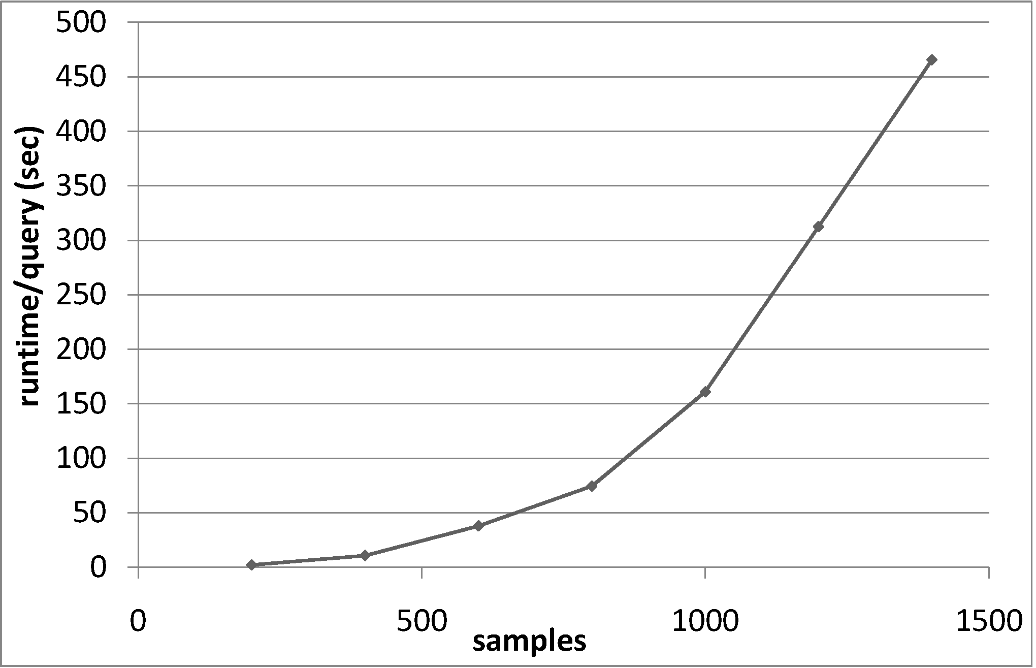
Figure 5: Runtime of MC for increasing sample size.

VII-A Runtime of the Monte-Carlo-based Approach

To the best of our knowledge, there exists no approach which is able to process uncertain similarity queries on probabilistic databases with continuous PDFs. A naive approach needs to consider all possible worlds and thus needs to integrate over all object PDFs, implying a runtime exponentially in the number of objects. Since this is not applicable even for small databases, we adapted an existing approach to cope with the conditions. The approach most related to our work is [21], which solves the problem of computing the domination count for a certain query and discrete distributions within the database objects. Thus the proposed comparison partner works as follows: Draw a sufficiently large number $S$ of samples from each object by Monte-Carlo-Sampling. Then, for each sample $q_{i}\in Q$ of the query, apply the algorithm proposed in [21] to compute an exact probabilistic domination count PDF of an object $B$. As proposed in [21], this is done using the generating function technique and using an and/xor tree to combine individual samples into discrete distributed uncertain objects. Finally, accumulate the resulting certain domination count PDFs of each $q_{i}\in Q$ into a single domination count PDF by taking the average. The execution time for this approach, which we will refer to as MC in the following, is shown in Figure 5. It can be observed that for a reasonable sample size (which is required to achieve a result that is close to the correct result with high probability) the runtime becomes very large.

Note that our comparison partner only works for discrete uncertain data (cf. Section VII-A). To make a fair comparison our approach relies on the same uncertainty model (default: 1000 samples/object). Nevertheless, all the experiments yield analogous results for continuous distributions.

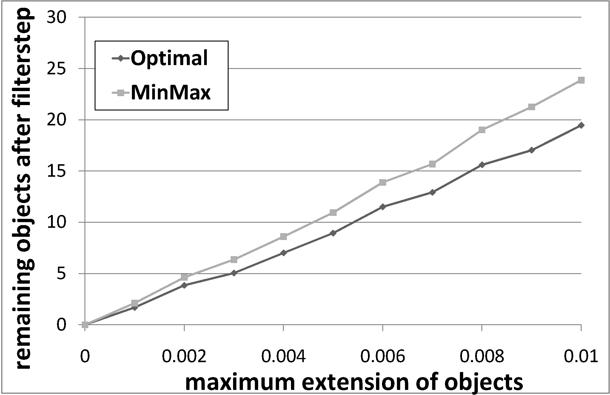
(a) Candidates after spatial pruning.

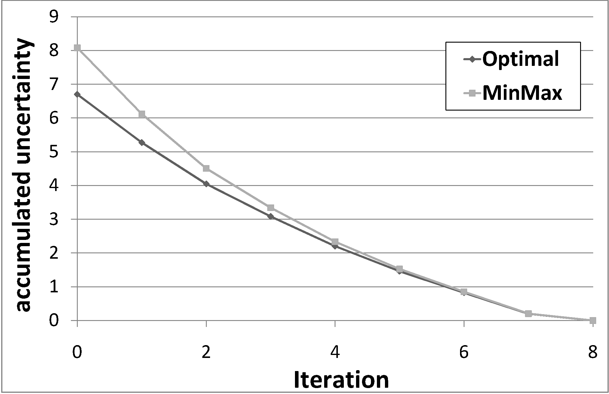
(b) Accumulated uncertainty of result.

Figure 6: Optimal vs. MinMax decision criterion.

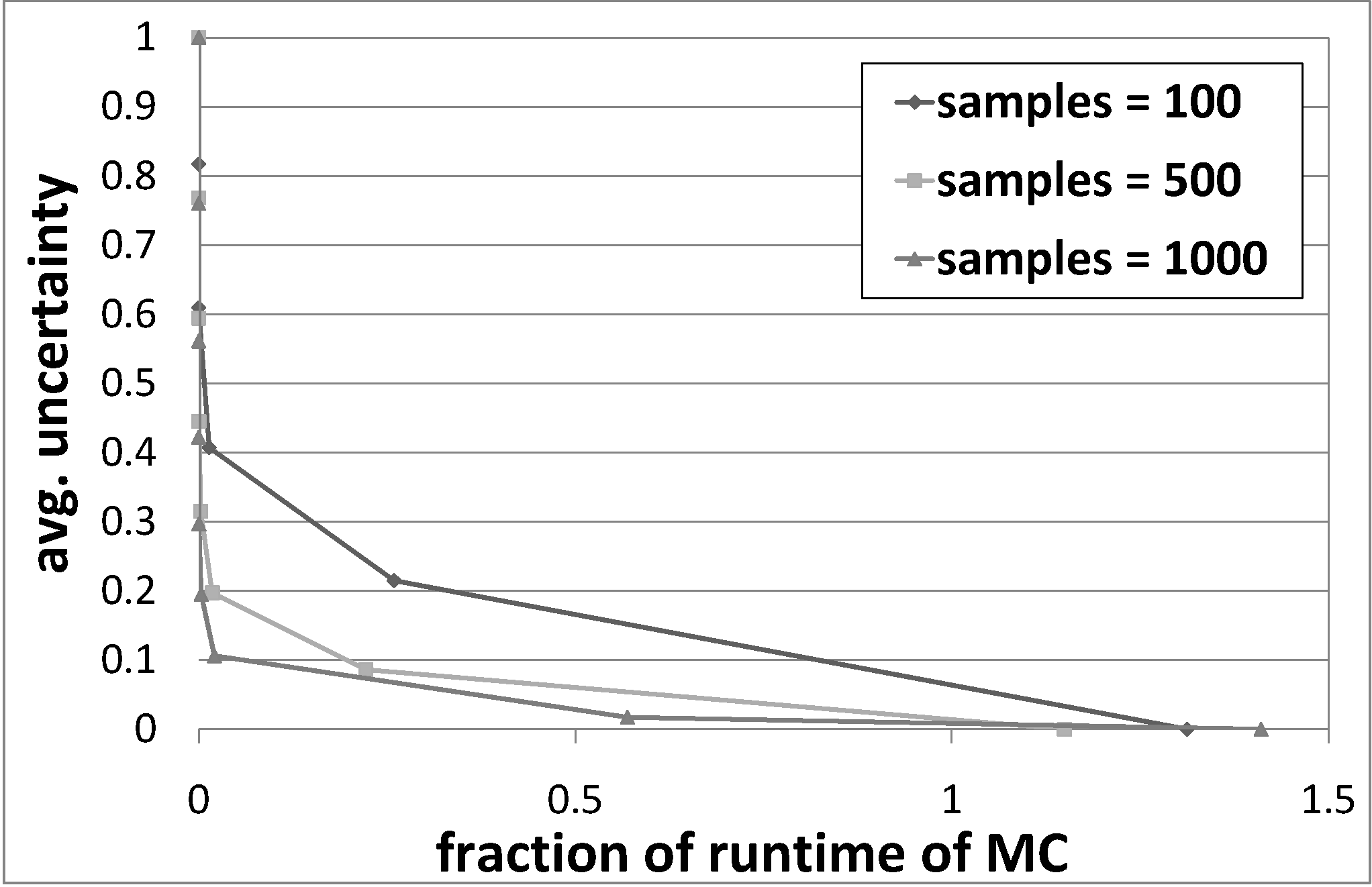
(a) Synthetic Data

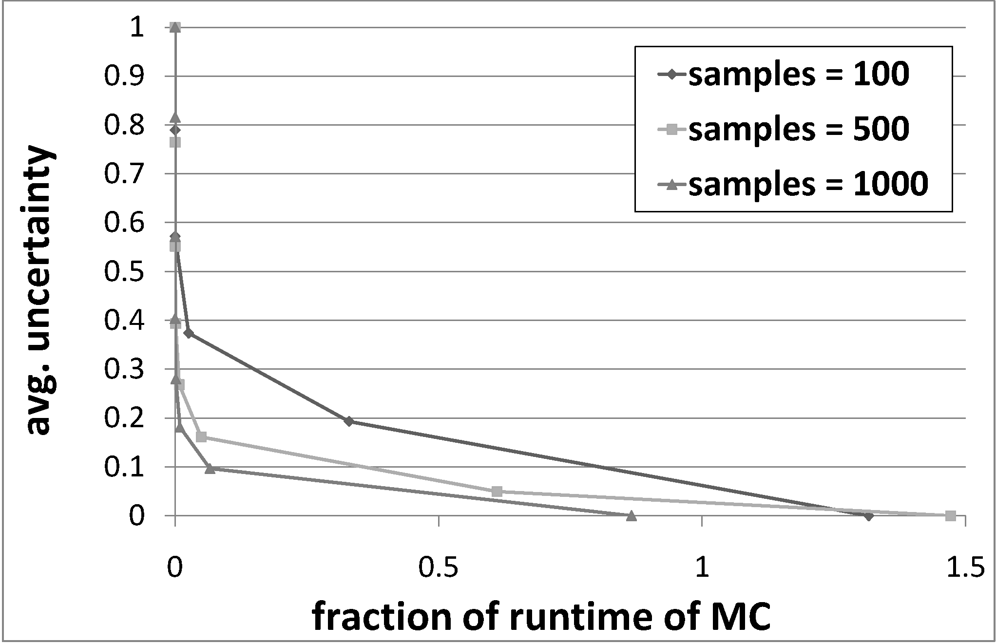
(b) Real Data

Figure 7: Uncertainty of IDCA w.r.t. the relative runtime to MC.

VII-B Optimal vs. Min/Max Decision Criterion

In the first experiment, we evaluate the gain of pruning power using the complete similarity domination technique (cf. Section III-A) instead of the state-of-the-art min/max decision criterion to prune uncertain objects from the search space. The first experiment evaluates the number of uncertain objects that cannot be pruned using complete domination only, that is the number of candidates are to evaluate in our algorithm. Figure 6(a) shows that our domination criterion (in the following denoted as optimal) is able to prune about 20% more candidates than the min/max pruning criterion. In addition, we evaluated the domination count approximation quality (in the remainder denoted as uncertainty) after each decomposition iteration of the algorithm, which is defined as the sum $\sum_{i=0}^{N}DomCount_{UB}^{i}(B,R)-DomCount_{LB}^{i}(B,R)$. The result is shown in Figure 6(b). The improvement of the complete domination (denoted as iteration $0$) can also be observed in further iterations. After enough iterations, the uncertainty converges to zero for both approaches.

VII-C Iterative Domination Count Approximation

Next, we evaluate the trade-off of our approach regarding approximation quality and the invested runtime of our domination count approximation. The results can be seen in Figure 7 for different sample sizes and datasets. It can be seen that initially, i.e. in the first iterations, the average approximation quality (avg. uncertainty of an influenceObject) decreases rapidly. The less uncertainty left, the more computational power is required to reduce it any further. Except for the last iteration (resulting in 0 uncertainty) each of the previous iterations is considerably faster than MC. In some cases (see Figure 7(b)) IDCA is even faster in computing the exact result.

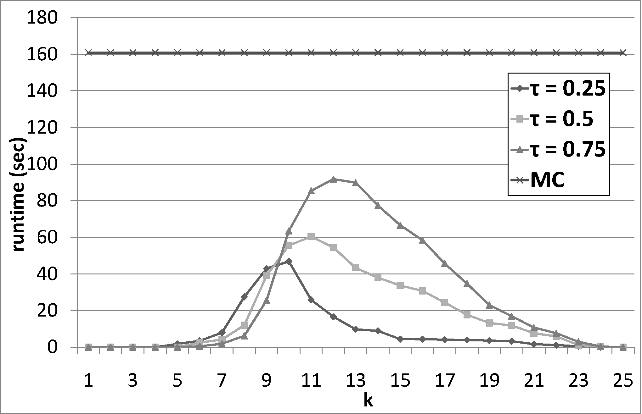
Figure 8: Runtimes of IDCA and MC for different query predicates $k$ and $\tau$.

VII-D Queries with a Predicate

Integrated in an application one often wants to decide whether an object satisfies a predicate with a certain probability. In the next experiment, we posed queries in the form: Is object $B$ among the $k$ nearest neighbors of $Q$ (predicate) with a probability of 25%, 50%, 75%? The results are shown in Figure 8 for various $k$-values. With a given predicate, IDCA is often able to terminate the iterative refinement of the objects earlier in most of the cases, which results in a runtime which is orders of magnitude below MC. In average the runtime is below MC in all settings.

VII-E Number of influenceObjects

The runtime of the algorithm is mainly dependent on the number of objects which are responsible for the uncertainty of the rank of $B$. The number of influenceObjects depends on the number of objects in the database, the extension of the objects and the distance between $Q$ and $B$. The larger this distance, the higher the number of influenceObjects. For the experiments in Figure 9(a) we varied the distance between $Q$ and $B$ and measured the runtime for each iteration. In Figure 9(b) we present runtimes for different sizes of the database. The maximum extent of the objects was set to 0.002 and the number of objects in the database was scaled from 20,000 to 100,000. Both experiments show that IDCA scales well with the number influencing objects.

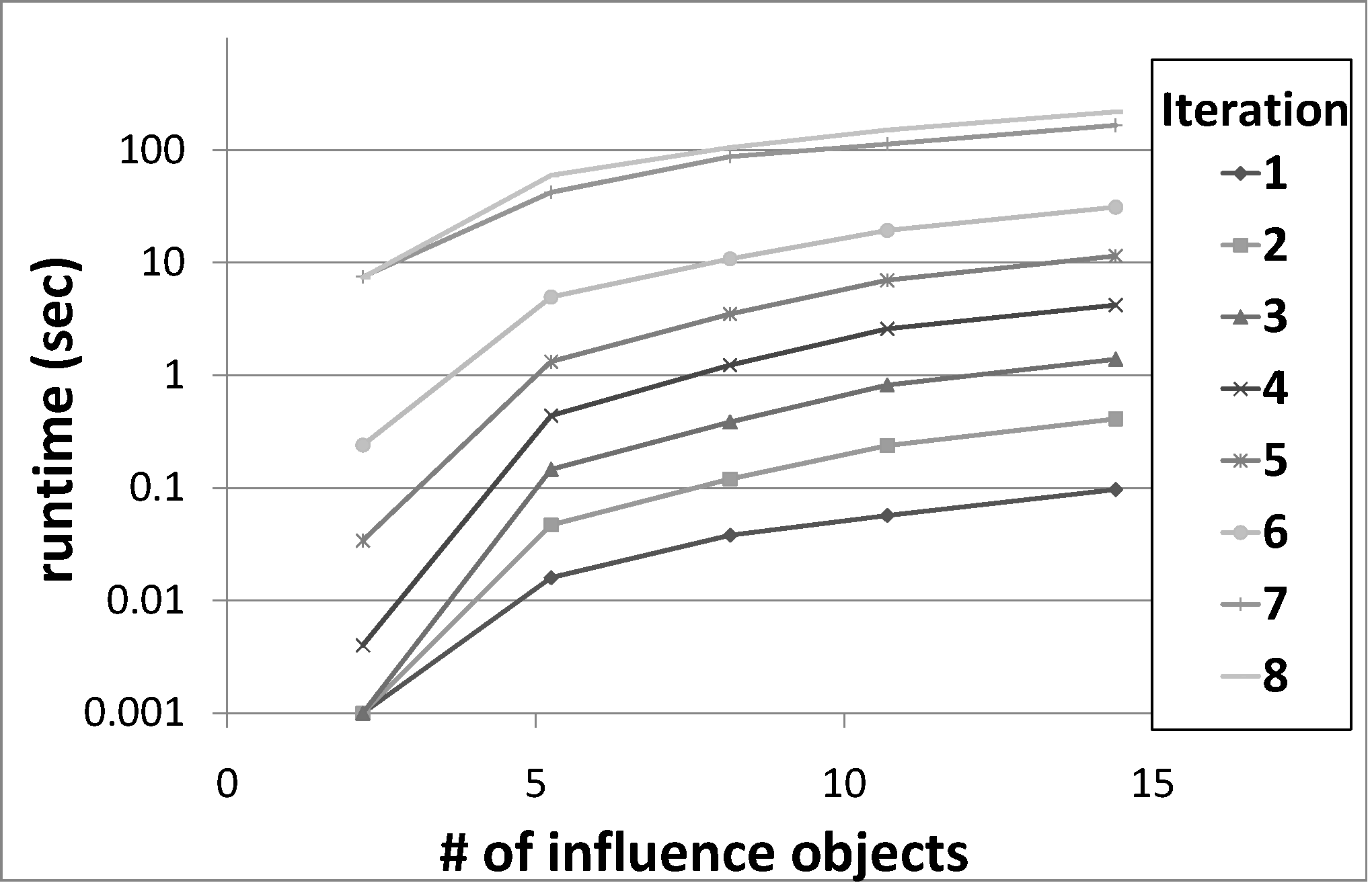
(a) Runtime w.r.t. number of influence objects.

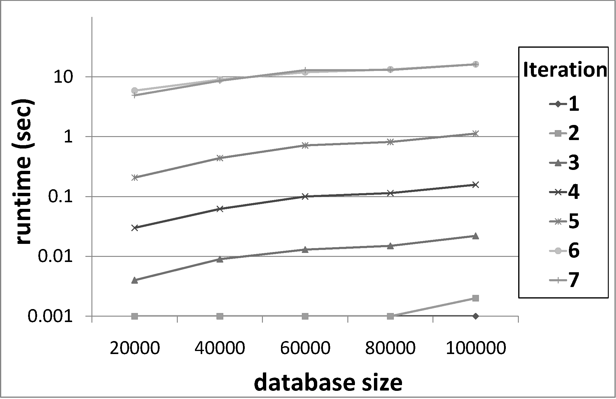
(b) Runtime for different sizes of the database.

Figure 9: Impact of influencing objects.

VIII Conclusions

In this paper, we applied the concept of probabilistic similarity domination on uncertain data. We introduced a geometric pruning filter to conservatively and progressively approximate the probability that an object is being dominated by another object. An iterative filter-refinement strategy is used to stepwise improve this approximation in an efficient way. Specifically we propose a method to efficiently and effectively approximate the domination count of an object using a novel technique of uncertain generating functions. We show that the proposed concepts can be used to efficiently answer a wide range of probabilistic similarity queries while keeping correctness according to the possible world semantics. Our experiments show that our iterative filter-refinement strategy is able to achieve a high level of precision at a low runtime. As future work, we plan to investigate further heuristics for the refinement process in each iteration of the algorithm. Furthermore we will integrate our concepts into existing index supported $k$NN- and R$k$NN-query algorithms.

References

- [1] L. Antova, T. Jansen, C. Koch, and D. Olteanu. Fast and simple relational processing of uncertain data. In Proc. ICDE, 2008.
- [2] J. L. Bentley. Multidimensional binary search trees used for associative searching. Commun. ACM, 18(9):509–517, 1975.
- [3] T. Bernecker, T. Emrich, H.-P. Kriegel, N. Mamoulis, M. Renz, and A. Z fle. A novel probabilistic pruning approach to speed up similarity queries in uncertain databases. http://www.dbs.ifi.lmu.de/Publikationen/Papers/ICDE2010_TR.pdf. Technical report.
- [4] T. Bernecker, H.-P. Kriegel, and M. Renz. Proud: Probabilistic ranking in uncertain databases. In Proc. SSDBM, pages 558–565, 2008.
- [5] T. Bernecker, H.-P. Kriegel, M. Renz, F. Verhein, and A. Züfle. Probabilistic frequent itemset mining in uncertain databases. In Proc. KDD, pages 119–128, 2009.
- [6] G. Beskales, M. A. Soliman, and I. F. IIyas. Efficient search for the top-k probable nearest neighbors in uncertain databases. Proc. VLDB Endow., 1(1):326–339, 2008.
- [7] M. A. Cheema, X. Lin, W. Wang, W. Zhang, and J. Pei. Probabilistic reverse nearest neighbor queries on uncertain data. IEEE Trans. Knowl. Data Eng., 22(4):550–564, 2010.
- [8] J. Chen and R. Cheng. Efficient evaluation of imprecise location-dependent queries. In Proc. ICDE, 2007.
- [9] R. Cheng, J. Chen, M. Mokbel, and C. Chow. Probabilistic verifiers: Evaluating constrained nearest-neighbor queries over uncertain data. In Proc. ICDE, 2008.
- [10] R. Cheng, L. Chen, J. Chen, and X. Xie. Evaluating probability threshold k-nearest-neighbor queries over uncertain data. In EDBT, pages 672–683, 2009.
- [11] R. Cheng, D. Kalashnikov, and S. Prabhakar. Querying imprecise data in moving object environments. In IEEE TKDE, 2004.
- [12] R. Cheng, S. Singh, and S. Prabhakar. U-dbms: a database system for managing constantly-evolving data. In Proc. VLDB, 2005.
- [13] R. Cheng, Y. Xia, S. Prabhakar, R. Shah, and J. Vitter. Efficient indexing methods for probabilistic threshold queries over uncertain data. In Proc. VLDB, pages 876–887, 2004.
- [14] G. Cormode, F. Li, and K. Yi. Semantics of ranking queries for probabilistic data and expected results. In Proc. ICDE, 2009.
- [15] T. Emrich, H.-P. Kriegel, P. Kröger, M. Renz, and A. Züfle. Boosting spatial pruning: On optimal pruning of mbrs. In Proc. SIGMOD, 2010.
- [16] M. Hua, J. Pei, W. Zhang, and X. Lin. Ranking queries on uncertain data: a probabilistic threshold approach. In Proc. SIGMOD, 2008.
- [17] Y. Iijima and Y. Ishikawa. Finding probabilistic nearest neighbors for query objects with imprecise locations. In Proc. MDM, 2009.
- [18] H.-P. Kriegel, P. Kunath, and M. Renz. Probabilistic nearest-neighbor query on uncertain objects. In DASFAA, pages 337–348, 2007.
- [19] J. Li, B. Saha, and A. Deshpande. A unified approach to ranking in probabilistic databases. PVLDB, 2(1):502–513, 2009.
- [20] X. Lian and L. Chen. Efficient processing of probabilistic reverse nearest neighbor queries over uncertain data. VLDB J., 18(3):787–808, 2009.
- [21] X. Lian and L. Chen. Probabilistic inverse ranking queries over uncertain data. In Proc. DASFAA, pages 35–50, 2009.
- [22] V. Ljosa and A. K. Singh. Apla: Indexing arbitrary probability distributions. In ICDE, pages 946–955, 2007.
- [23] P. Sen and A. Deshpande. Representing and querying correlated tuples in probabilistic databases. In Proc. ICDE, 2007.
- [24] S. Singh, C. Mayfield, S. Mittal, S. Prabhakar, S. E. Hambrusch, and R. Shah. Orion 2.0: native support for uncertain data. In Proc. SIGMOD, pages 1239–1242, 2008.
- [25] M. Soliman and I. Ilyas. Ranking with uncertain scores. In Proc. ICDE, pages 317–328, 2009.
- [26] Y. Tao, R. Cheng, X. Xiao, W. K. Ngai, B. Kao, and S. Prabhakar. Indexing multi-dimensional uncertain data with arbitrary probability density functions. In Proc. VLDB, 2005.
- [27] O. Wolfson, A. P. Sistla, S. Chamberlain, and Y. Yesha. Updating and querying databases that track mobile units. Distributed and Parallel Databases, 7(3):257–387, 1999.