Density functional theory beyond the linear regime: Validating adiabatic LDA

Abstract

We present a local density approximation (LDA) for one-dimensional (1D) systems interacting via the soft-Coulomb interaction based on quantum Monte-Carlo calculations. Results for the ground-state energies and ionization potentials of finite 1D systems show excellent agreement with exact calculations, obtained by exploiting the mapping of an $N$-electron system in $d$ dimensions, onto a single electron in $N\times d$ dimensions properly symmetrized by the Young diagrams. We conclude that 1D LDA is of the same quality as its three-dimensional (3D) counterpart, and we infer conclusions about 3D LDA. The linear and non-linear time-dependent responses of 1D model systems using LDA, exact exchange, and the exact solution are investigated and show very good agreement in both cases, except for the well known problem of missing double excitations. Consequently, the 3D LDA is expected to be of good quality beyond linear response. In addition, the 1D LDA should prove useful in modeling the interaction of atoms with strong laser fields, where this specific 1D model is often used.

Over the last years the theoretical description of optical properties of complex many-electron systems, from molecules, to nanostructures and extended systems, has re-flourished due to the efficient implementation of time-dependent density-functional theory (TDDFT) RG1984 ; TDDFT2006 . The good performance shown by the adiabatic local density approximation (ALDA) for many finite systems has limited the development of exchange-correlation (xc) functionals with a more elaborate time-dependence, which is clearly in its infancy compared to static DFT. However recently many important deficiencies, especially of the adiabatic approximation, have been identified ORR2002 ; MBW2002 ; MZCB2004 ; DH2004 ; M2005 ; BWG2005 ; VMR2008 ; CCJ2009 ; GMG2009 ; GB2009 .

Ultrafast time-resolved optical spectroscopy has revealed new classes of physical, chemical, and biological reactions, in which directed, deterministic motions of atoms have a key role. The advent of free electron lasers with attosecond resolution increases the capabilities of present femtosecond pump-probe experiments, allowing for a study of the dynamics of non-equilibrium electronic systems in real time. In addition, systems of all sizes can be investigated, from the atomic scale to the most extended molecules (e.g. DNA, proteins and their complexes) and solids. Despite those tremendous experimental advances, the theoretical description of a real molecular system subject to ultrashort, intense, and/or high-frequency lasers is still in a fledgeling state. Several problems need to be addressed, ranging from the non-perturbative nature of the physical processes involved to the simultaneous description of the (interacting) electronic and nuclear degrees of freedom. Therefore, it is of paramount relevance to have a theoretical framework which allows for a non-perturbative description of electrons, and at the same time is able to tackle electron-ion dynamics in the excited-state. TDDFT seems to be the suitable framework to move the realm of density-functional methods beyond the linear regime to describe the aformentioned processes. One important advantage is the combined electron and ion dynamics provided by TDDFT TDDFT2006 .

Many physical processes rely on the knowledge of non-linear response functions. Therefore, it is very timely to provide a systematic study addressing the performance of present functionals in the non-linear regime. To assess the quality of a functional we need to have appropriate data for comparison. Obtaining accurate experimental data in the non-linear regime can be very difficult for real systems, due to various limitations, e.g. solvent effects or additional approximations going into the interpretation of the collected data SMBWRSD1993 ; KDS1998 . These problems can be avoided by using exactly solvable models which then allow for a direct comparison between the exact spetrum and an approximate one. Unfortunately, an exact propagation of even small three-dimensional systems is computationally very demanding, and needs further simplification. One possibility is the reduction of dimensionality, i.e. the use of one-dimensional (1D) models, where the exact diagonalization is feasible as long as the number of electrons is sufficiently small. In the present paper we work with systems of interacting electrons in 1D. Having the exact solution allows us to test orbital dependent functionals such as exact exchange (EXX) which can be easily transferred to different dimensions. A local density approximation (LDA) is achieved, as in the 3D case, by quantum Monte-Carlo (QMC) studies of the homogeneous reference, and parametrizing the corresponding correlation energy.

The present work, besides adding fundamental information concerning the relevance of spatial and time non-locality in the xc functional, also provides a proper LDA parametrization for electrons interacting via the soft-Coulomb interaction in 1D systems. This model description is widely used in the context of high-intensity lasers, where above-threshold ionization and high-harmonic generation play an important role JES1988 ; E1990 ; LGE2000 ; L2005 . Also, 1D two-electron systems are employed to gain insight into exact properties of the xc potential and kernel in static and time-dependent density functional theory, since these systems can easily be solved exactly TGK2008 ; TMM2009 ; HTR2009 .

The 1D Hamiltonian for $N$ particles moving in a general external potential $v_{ext}$ reads

$$H=\sum_{j=1}^{N}\left[-\frac{1}{2}\frac{d^{2}}{dx_{j}^{2}}+v_{ext}(x_{j})\right]+\frac{1}{2}\sum_{\stackrel{{\scriptstyle\scriptstyle j,k=1}}{{j\neq k}}}^{N}v_{int}(x_{j},x_{k}),$$ (1)

where $v_{int}$ describes the electron-electron interaction. In order to avoid the singularity of the Coulomb interaction we employ the soft-Coulomb potential

$$v_{soft-C}(x_{1},x_{2})=\frac{q_{1}q_{2}}{\sqrt{a^{2}+(x_{1}-x_{2})^{2}}}$$ (2)

instead. Here, $q_{1}$ and $q_{2}$ describe the charges of the particles while $a$ is the usual softening parameter (atomic units $e=m=\hbar=1$ are used throughout this paper). Unless stated explicitly, we use $a=1$ for all our calculations. Mathematically, it is straightforward to show that the Hamiltonian (1) is equivalent to a single particle in $N$ dimensions, moving in an external potential consisting of all the contributions from $v_{ext}$ and $v_{int}$. The corresponding Schrödinger equation can, hence, be solved by any code which is able to treat non-interacting particles in the correct number of dimensions in an arbitrary external potential. Due to the Hamiltonian being symmetric under particle interchange, $x_{j}\leftrightarrow x_{k}$, the solutions of the Schrödinger equation can be chosen as symmetric or antisymmetric under such an exchange. For the simplest case of two interacting electrons both the symmetric and antisymmetric solutions are valid, corresponding to the singlet and triplet spin configurations, respectively. However, for more than two electrons one needs to separately ensure that the spatial wave function is a solution to the $N$-electron problem. For example, a totally symmetric spatial wave function is a correct solution for a single particle in $N$ dimensions, however, for $N>2$ there is no corresponding spin function such that the total wave function has the required antisymmetry to be a solution of the $N$ fermion problem in 1D. We solve this problem by symmetrizing the solutions according to all possible fermionic Young diagrams for the given particle number $N$ LL1977 . The solution of higher dimensional problems within these symmetry restrictions has been implemented into the OCTOPUS computer program MCBR2003 ; CAORALMGR2006 . Usually, the lowest energy solution is found to be purely symmetric and is discarded for $N>2$. With increasing number of electrons we also observe an increasing number of states which do not satisfy the fermionic symmetry requirements.

As a result of reducing the number of dimensions, we need to use an appropriate functional for performing the DFT calculations. While any orbital functional can easily be transferred between dimensions, those functionals based on specific systems need to be recalculated. This affects the most common functional, i. e. the local density approximation, available only for the normal Coulomb interaction in two and three dimensions AMGB2002 ; KS1965 , an effective Coulomb interaction of a harmonically confined wire CSS2006 ; SCSM2009 , and some other ad-hoc 1D models XPTCCR2006 ; XPAT2006 ; XA2008 . In this work, we present and use a parametrization of the 1D LDA obtained from quantum Monte-Carlo simulations, which are exact in 1D, using the soft-Coulomb interaction in Eq. 2. We assess the quality of the approximation in calculating ground-state properties as well as the linear response for various 1D model systems. We then proceed to calculate the nonlinear response and compare the exact one with the ALDA and adiabatic exact-exchange (AEXX) spectra.

The correlation energy of the LDA is parametrized in terms of $r_{s}$ and the spin polarization $\zeta=(N_{\uparrow}-N_{\downarrow})/N$ in the form

$$\epsilon_{c}(r_{s},\zeta)=\epsilon_{c}(r_{s},\zeta=0)+\zeta^{2}\left[\epsilon_{c}(r_{s},\zeta=1)-\epsilon_{c}(r_{s},\zeta=0)\right]$$ (3)

with

$$\epsilon_{c}(r_{s},\zeta=0,1) = -\frac{1}{2}\frac{r_{s}+Er_{s}^{2}}{A+Br_{s}+Cr_{s}^{2}+Dr_{s}^{3}}$$ (4)

$$\times\ln(1+\alpha r_{s}+\beta r_{s}^{m}),$$

which proved to be very accurate in the parametrization for other 1D systems with a different long-range interaction CSS2006 . Note that the additional factor of $1/2$ is due the use of Hartree atomic units, as everywhere else in the paper. To obtain the exact high-density result, known from the random phase approximation SCSM2009 , i.e.

$$\epsilon_{c}(r_{s}\rightarrow 0,\zeta=0) = -4/(\pi^{4}a^{2})~{}r_{s}^{2},$$ (5)

$$\epsilon_{c}(r_{s}\rightarrow 0,\zeta=1) = -1/(2\pi^{4}a^{2})~{}r_{s}^{2}$$ (6)

to leading order in $r_{s}$, we fix the ratio $\alpha/A$ to be equal to $8/(\pi^{4}a^{2})$ and $1/(\pi^{4}a^{2})$ for $\zeta=0$ and $\zeta=1$, respectively. In both cases the exponent $m$ is limited to values larger than 1. As a result, the number of independent parameters in the function (4) is reduced to 7. In addition, for $a=1$ the denominator can be simplified by setting $B=0.0$. However, for smaller values of the softening parameter $a$ the linear term in the denominator is important for achieving better agreement with the quantum Monte Carlo results.

	$a=1.0$		$a=0.5$
	$\zeta=0$	$\zeta=1$	$\zeta=0$
$A$	18.40(29)	5.24(79)	7.40(18)
$B$	0.0	0.0	1.120(119)
$C$	7.501(39)	1.568(230)	1.890(63)
$D$	0.10185(5)	0.1286(150)	0.0964(108)
$E$	0.012827(10)	0.00320(74)	0.0250(23)
$\alpha$	1.511(24)	0.0538(82)	2.431(62)
$\beta$	0.258(6)	$1.56(1.31)\cdot 10^{-5}$	0.0142(25)
$m$	4.424(25)	2.958(99)	2.922(83)
av. error	$6.7\cdot 10^{-5}$	$3.3\cdot 10^{-5}$	$7.7\cdot 10^{-4}$

Table 1: Values of the LDA correlation energy parametrization in Eq. 4. For the most widely used case, i.e. $a=1$, the parametrization is reported for both unpolarized ($\zeta=0$) and fully polarized ($\zeta=1$) systems. The error on the last digits is given in parenthesis, while the average error (in Hartree) in the full density range is given in the last row.

The optimal values of the parameters for $a=1$ and $a=0.5$ are reported in Tab. 1, and implemented in the OCTOPUS program MCBR2003 ; CAORALMGR2006 . For more details on the 1D QMC methodology and the parametrization procedure we refer to Refs. CSS2006, ; SCSM2009, .

	$E_{\mathrm{total}}$			IP
	Exact	LDA	SLDA	Exact	(S)LDA	$\epsilon_{\mathrm{HOMO}}^{\mathrm{(S)LDA}}$
H	-0.67	-0.60	-0.65	0.67	0.65	-0.41
He	-2.24	-2.20		0.75	0.75	-0.48
Li	-4.21	-4.16	-4.18	0.31	0.33	-0.18
Be	-6.78	-6.76		0.33	0.35	-0.16
He+	-1.48	-1.41	-1.45	1.48	1.45	-1.18
Li+	-3.90	-3.85		1.56	1.55	-1.24
Be+	-6.45	-6.39	-6.41	0.83	0.85	-0.63
Li2+	-2.34	-2.25	-2.30	2.34	2.30	-2.00
Be2+	-5.62	-5.56		2.41	2.38	-2.06
Be3+	-3.21	-3.13	-3.18	3.21	3.18	-2.86

Table 2: Total energies and ionization potentials for one-dimensional atoms and ions from exact and (spin-)LDA calculations as well as the eigenvalues of the highest occupied Kohn-Sham orbital. All numbers are given in Hartree.

As a first test, we calculated the ground-state energies of small atomic systems, for example, a 1D helium atom with $q=2$ in Eq. (2) and two electrons which interact via the soft Coulomb interaction. The ground state energies and ionization potentials from the exact and unpolarized LDA calculations are given in Tab. 2. We include all possible systems with one, two, three and four electrons in our test. For open-shell systems, we additionally performed a spin-DFT (SLDA) calculation, where the xc energy was spin dependent according to Eq. (3). All atomic calculations were performed in a box ranging from -8 to 8 bohr with a spacing of 0.2 bohr, which ensures the total energy to be converged to the accuracy stated in the table.

As we can see, the LDA total energies for the neutral and positively charged systems agree very well with the exact results. As expected, the spin-resolved calculations further improve the agreement for the open-shell systems. As a result, the ionization potentials, calculated as the difference of the total energies of the $N$ and the $N-1$ electron systems, from the (S)LDA and the exact calculations agree almost perfectly. The largest Kohn-Sham eigenvalue $\epsilon_{HOMO}^{(S)LDA}$ only partially accounts for the total ionization potential, i.e. the 1D LDA violates this known property of the exact functional AB1985b . The good agreement for the positively charged systems is not reproduced for negatively charged ones. For the small systems investigated here, LDA does not bind an extra electron while the exact calculation shows that the negatively charged systems are indeed stable giving total energies of $-0.73$ Ha, $-2.35$ Ha and $-4.17$ Ha for H^-, He^-, and Li^-, respectively. A comparison with the total energies of the neutral systems shows that in the exact calculation the additional electron is only very lightly bound in 1D. It is no surprise that the LDA, with its usual wrong asymptotic behavior of the exchange-correlation potential, does not yield stable negatively charged ions.

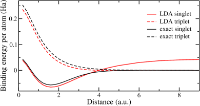
Figure 1: Binding energy per atom of the one-dimenstional hydrogen molecule as a function of the distance between the two ions, exact and LDA calculations for the singlet ground state and the first triplet state.

As a second test of the new functional we calculate the dissociation curve of the 1D hydrogen molecule. For these calculations we increased the size of the simulation box to range from -20 to 20 bohr in order to achieve convergence also for the stretched molecule. Fig. 1 shows the binding energy per atom as a function of the distance between the two ions. As one can see, the known pathology of 3D LDA is reproduced also in 1D. The singlet state yields a good description around the equilibrium distance of $1.6$ bohr with the binding energy being slightly overestimated by LDA. However, the bond breaking is not described correctly due to the strong static correlation at large distances. The LDA calculation for the triplet state yields very good agreement over the whole range of distances corroborating the general experience of LDA performing better for more polarized systems.

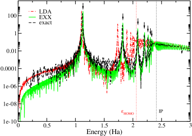
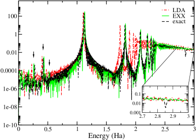
Figure 2: Linear (top) and non-linear (bottom) spectra of Be²⁺ comparing the exact and the 1D LDA calculation. The inset in the bottom figure shows a zoom into the region from $2.7$ to $3.0$ Ha.

	$\omega_{1}$	$\omega_{2}$	$\omega_{3}$	$\omega_{4}$	$\omega_{5}$	$\omega_{6}$	$\omega_{7}$	$\Omega_{1}$	$\Omega_{2}$	$\Omega_{3}$
LDA	1.10	1.74	1.90	1.96	2.00	-	-	0.22	0.40	-
EXX	1.13	1.82	2.08	2.20	2.27	2.30	2.32	0.26	0.43	0.52
exact	1.12	1.81	2.08	2.19	2.26	2.29	2.32	0.28	0.42	0.54

Table 3: Excitation energies from linear and non-linear response of the 1D Be²⁺ atom corresponding to the spectra in Fig. 2. Excitations from linear response are denoted as $\omega$ while those from the non-linear spectrum are denoted with $\Omega$. All numbers are given in Hartree.

After having shown that the 1D LDA behaves very much like its 3D counterpart for ground-state calculations, we turn our attention to TDDFT where we use it as an adiabatic approximation to the exact time-dependent exchange-correlation potential. The propagations were performed in a box ranging from -150 to 150 bohr with absorbing boundary conditions MCBR2003 and a grid spacing of 0.2 bohr for a total propagation time of $10^{3}$ a.u.

In Fig. 2 we compare the spectra calculated in a linear and non-linear regime from the exact and the LDA calculations for a Be²⁺ system, i.e. a positive charge with $q=4$ and 2 interacting electrons in a singlet configuration. In the linear regime a kick of $10^{-4}$ Ha/bohr was employed at $t=0$ which was then increased to $0.01$ Ha/bohr to obtain the non-linear response. The values of the excitation energies can be found in Tab. 3. In linear response, we see five peaks in the LDA spectrum which compare well with the first five excitations in the exact case. As expected, the agreement is better for lower lying excitations and gets worse the closer we get to the continuum. As a guide for the eye we included the KS HOMO energy of the LDA calculation and the exact ionization potential. The onset of the continuum itself appears at too low energies in the LDA calculation missing two more clearly visible peaks in the exact spectrum. In other words, the LDA fails to reproduce the proper Rydberg series, a behavior well known from 3D calculations. For comparison we also included the results from an EXX calculation which shows a slightly better agreement than LDA for the first three excitations but, more importantly, reproduces the Rydberg series due to the correct asymptotic behavior of the corresponding exchange potential. The quality of the EXX results also implies that correlation is of secondary importance in the system for $a=1$. The non-linear spectrum shows the same excitations as the linear spectrum and three additional peaks for the exact and the EXX calculation and two additional peaks in the LDA spectrum. Their energies are also listed in Tab. 3. Due to the spatial symmetry of the system all even order responses are zero and the first non-vanishing higher-order response is of third order. The $\Omega_{1}=0.28$ Ha corresponds to an excitation from the second to the third excited state, where the transition from the ground to the second excited state is dipole forbidden and, hence, can only be reached in a two-photon process. The other two frequencies, $\Omega_{2}=0.42$ Ha and $\Omega_{3}=0.54$ Ha, correspond to the transitions from first to second and second to fifth excited state, respectively. Again, both the EXX and the LDA calculations yield a good description of the low lying excitations, only the third peak cannot be resolved in the LDA spectrum.

One feature of the exact spectrum that is missing from both the LDA and the EXX spectra is the small dip at 2.8 Ha, see inset in Fig. 2. It results from a Fano resonance F1961 ; FC1968 , i.e. the decay of an excited state into continuum states. It is missing from both approximate spectra due to the double-excitation character of the involved excited state. Double excitations can only be described in TDDFT if a frequency-dependent xc kernel is employed MZCB2004 . Any adiabatic approximation, however, leads to a frequency independent kernel. Hence, double excitations, as well as any resulting features, are missing from both the ALDA and the AEXX calculations. Apart from the well-known shortcomings of not including double-excitations and not giving the correct Rydberg series, the 1D ALDA reproduces both the linear and the non-linear exact spectra quite well.

We have introduced a one-dimensional LDA suitable for the description of systems interacting via the commonly used soft-Coulomb interaction. We have shown that the one-dimensional functional is of the same quality as its three-dimensional counterpart in the calculation of ground-state energies of atomic systems and the dissociation of small molecules. Also, the linear spectra show the same quality known from 3D calculations with low energy excitations being well described while Rydberg and double excitations are missing. Generally, for the 1D LDA one can expect the same success and failure in applications that are known from 3D calculations, i.e. the quality of the LDA results appears to be independent of the dimensionality. We emphasize that the 1D LDA yields a good description not only in linear response but also in the non-linear case. Consequently, one can expect 3D LDA calculations to perform well for the calculation of non-linear response, where the experimental data is often difficult to interpret.

The reduced dimensionality of the model systems treated in this work allows for a direct solution of the interacting problem for small number of particles. The comparison between the DFT and an exact calculation allows for an assessment of the quality of approximations beyond what is possible in three-dimensional systems. One-dimensional model systems can provide useful insight which hopefully will allow for the construction of new functionals in the future.

We acknowledge funding by the Spanish MEC (FIS2007-65702-C02-01), ACI-promciona project (ACI2009-1036), “Grupos Consolidados UPV/EHU del Gobierno Vasco” (IT-319-07), and the European Community through e-I3 ETSF project (Contract No. 211956).

References

- (1) E. Runge and E. K. U. Gross, Phys. Rev. Lett. 52, 997 (1984).
- (2) Time-Dependent Density Functional Theory, Vol. 706 of Lecture Notes in Physics, edited by M. A. L. Marques et al. (Springer Berlin / Heidelberg, 2006).
- (3) G. Onida, L. Reining, and A. Rubio, Rev. Mod. Phys. 74, 601 (2002).
- (4) N. T. Maitra, K. Burke, and C. Woodward, Phys. Rev. Lett. 89, 023002 (2002).
- (5) N. T. Maitra, F. Zhang, R. Cave, and K. Burke, J. Chem. Phys. 120, 5932 (2004).
- (6) A. Dreuw and M. Head-Gordon, J. Am. Chem. Soc. 126, 4007 (2004).
- (7) N. Maitra, J. Chem. Phys. 122, 234104 (2005).
- (8) K. Burke, J. Werschnik, and E. K. U. Gross, J. Chem. Phys. 123, 062206 (2005).
- (9) D. Varsano, A. Marini, and A. Rubio, Phys. Rev. Lett. 101, 133002 (2008).
- (10) TDDFT for Molecules and Molecular Solids, edited by M. Casida, H. Chermette, and D. Jacquemin (Special Issue in Journal of Molecular Structure: THEOCHEM, vol.914, Issues 1-3 2009).
- (11) L. Goerigk, J. Moellmann, and S. Grimme, Phys. Chem. Chem. Phys. 11, 4611 (2009).
- (12) O. Gritsenko and E. Baerends, Phys. Chem. Chem. Phys. 11, 4640 (2009).
- (13) M. Stahelin et al., J. Chem. Phys. 98, 5595 (1993).
- (14) P. Kaatz, E. Donley, and D. Shelton, J. Chem. Phys. 108, 849 (1998).
- (15) J. Javanainen, J. Eberly, and Q. Su, Phys. Rev. A 38, 3430 (1988).
- (16) J. Eberly, Phys. Rev. A 42, 5750 (1990).
- (17) M. Lein, E. K. U. Gross, and V. Engel, Phys. Rev. Lett. 85, 4707 (2000).
- (18) M. Lein, Phys. Rev. A 72, 053816 (2005).
- (19) M. Thiele, E. K. U. Gross, and S. Kümmel, Phys. Rev. Lett. 100, 153004 (2008).
- (20) D. G. Tempel, T. J. Martínez, and N. T. Maitra, J. Chem. Theory and Computation 5, 770 (2009).
- (21) N. Helbig, I. Tokatly, and A. Rubio, J. Chem. Phys. 131, 224105 (2009).
- (22) L.D. Landau and E.M. Lifschitz, Quantum Mechanics (Butterworth-Heinemann, Oxford, 1977).
- (23) M. A. L. Marques, A. Castro, G. F. Bertsch, and A. Rubio, Comp. Phys. Comm. 151, 60 (2003).
- (24) A. Castro et al., Phys. Stat. Sol. (b) 243, 2465 (2006).
- (25) C. Attaccalite, S. Moroni, P. Gori-Giorgi, and G. B. Bachelet, Phys. Rev. Lett. 88, 256601 (2002).
- (26) W. Kohn and L. J. Sham, Phys. Rev. 140, A1133 (1965).
- (27) M. Casula, S. Sorella, and G. Senatore, Phys. Rev. B 74, 245427 (2006).
- (28) L. Shulenburger, M. Casula, G. Senatore, and R. Martin, J. Phys. A: Math. Theor. 42, 214021 (2009).
- (29) G. Xianlong et al., Phys. Rev. B 73, 165120 (2006).
- (30) G. Xianlong, M. Polini, R. Asgari, and M. P. Tosi, Phys. Rev. A 73, 033609 (2006).
- (31) G. Xianlong and R. Asgari, Phys. Rev. A 77, 033604 (2008).
- (32) C.-O. Almbladh and U. von Barth, Phys. Rev. B 31, 3231 (1985).
- (33) U. Fano, Phys. Rev. 124, 1866 (1961).
- (34) U. Fano and J. W. Cooper, Rev. Mod. Phys. 40, 441 (1968).