Interaction-enhanced double resonance in cold gases

Abstract

A new type of double-resonance spectroscopy of a quantum gas based on interaction-induced frequency modulation of a probe transition has been considered. Interstate interaction of multilevel atoms causes a coherence-dependent collisional shift of the transition between the atomic states $|1\rangle$ and $|2\rangle$ due to a nonzero population of the state $|3\rangle$. Thus, the frequency of the probe transition $|1\rangle-|2\rangle$ experiences oscillations associated with the Rabi oscillations between the states $|1\rangle$ and $|3\rangle$ under continuous excitation of the drive resonance $|1\rangle-|3\rangle$. Such a dynamic frequency shift leads to a change in the electromagnetic absorption at the probe frequency and, consequently, greatly enhances the sensitivity of double-resonance spectroscopy as compared to traditional “hole burning”, which is solely due to a decrease in the population of the initial state $|1\rangle$. In particular, it has been shown that the resonance linewidth is determined by the magnitude of the contact shift and the amplitude of the drive field and does not depend on the static field gradient. The calculated line shape and width agree with the low-temperature electron-nuclear double-resonance spectra of two-dimensional atomic hydrogen.

1 Introduction

Interaction of atoms and, more specifically, short-range or contact interaction, leads to a shift of internal atomic transitions commonly referred to as a contact shift. In the case of multi-level atoms, the contact shift also depends on interstate coherence and populations of the states not involved in the particular resonance. More specifically, according to experiments on ⁶Li Gupta and ⁴⁰K Regal_Jin and recent theory Baym ; Saf_JLTP , an incoherent population of such a third state causes a nonzero shift for fermions. On the other hand, fermions in identical internal states do not interact via $s$ waves; therefore, a fully coherent ultra-cold Fermi gas exhibits a contact shift only in the case of spatial inhomogeneity Campbell ; Gibble . On the contrary, the respective contribution to the contact shift of bosons is the highest if the internal states are coherently populated and decreases by a factor of 2 as the sample decoheres. Thus, in a Bose gas, excitation of a drive transition to the state $|3\rangle$ induces frequency modulation of the probe transition $|1\rangle-|2\rangle$ associated with Rabi oscillations between the states $|1\rangle$ and $|3\rangle$ Saf_JLTP . The latter leads to interaction-enhanced double resonance when two transitions are excited simultaneously. In this work, we consider this effect in the relaxation-free approximation, analyze a possible double-resonance lineshape and compare it with experiments in spin-polarized atomic hydrogen Ahokas ; Ahokas_JLTP .

Interaction of multilevel systems with several resonance fields is commonly considered with the use of the evolution equations for the components of spin density matrix CPT . Inclusion of the population-dependent frequency shift makes these equations essentially nonlinear and their analytical solution impossible. Our approach is less comprehensive but provides quantitative and physically clear description in the case of interest.

2 Interaction-enhanced double resonance

Physics of this novel phenomenon becomes transparent already in the case of just three levels (Fig. 1). In general, excitation of the probe transition $|1\rangle-|2\rangle$ affects the frequency of the drive $|1\rangle-|3\rangle$ resonance and vise versa. This may lead to specific effects and produce peculiar double-resonance spectra, which will be considered elsewhere.

Here, for simplicity and clarity, we restrict ourselves to the case (see below for the exact condition) when the contact shift vanishes in the absence of the third state. Another advantage of this case is that it allows direct comparison with experiments on electron-nuclear double resonance (ENDOR) in atomic hydrogen Ahokas ; Ahokas_JLTP . To simplify our consideration even further, we assume that the population of the state $|2\rangle$, which is the final state of the probe transition, is kept negligibly small and therefore the frequency of the drive transition remains constant. On the other hand, the frequency shift of the probe transition $|1\rangle-|2\rangle$ in the presence of the state $|3\rangle$ is Saf_JLTP

$$\hbar\Delta\omega^{\rm Bose}_{12(3)} = 2n_{1}(\lambda^{+}_{12}-\lambda_{11})+2n_{2}(\lambda_{22}-\lambda^{+}_{12})$$ (1)

$$+ 2n_{3}|C^{+}_{13}|^{2}(\lambda^{+}_{23}-\lambda^{+}_{13}),$$

$$\hbar\Delta\omega^{\rm Fermi}_{12(3)} = 2n_{3}|C^{-}_{13}|^{2}(\lambda^{-}_{23}-\lambda^{-}_{13}).$$ (2)

Here, $n_{i}$ is the population of the state $|i\rangle$, $\lambda^{\pm}_{ij}\equiv\langle ij|\lambda|ij\rangle_{\pm}$ is the matrix element (excluding the spatial factor) of the interaction strength $\lambda=4\pi\hbar^{2}a/m$ commonly used in a cold-collision regime, $m$ is the atomic mass, and $a$ is the respective scattering length. $C_{ij}^{\pm}$ are the normalized ($|C_{ij}^{+}|^{2}+|C_{ij}^{-}|^{2}=1$) amplitudes of the (+) symmetric and ($-$) antisymmetric component of properly symmetrized diatomic wavefunction $|{\bf k}i,{\bf q}j\rangle=C_{ij}^{+}\psi_{\pm}|ij\rangle_{+}+C_{ij}^{-}\psi_{\mp}|ij\rangle_{-}$, where the upper (lower) subscript stands for bosons (fermions) and the internal (pseudo-spin) and spatial parts are, respectively, $|ij\rangle_{\pm}=\frac{1}{\sqrt{2}}(|ij\rangle\pm|ji\rangle)$ and $\psi_{\pm}=\frac{1}{\sqrt{2}}(\psi_{\bf k}({\bf r}_{1})\psi_{\bf q}({\bf r}_{2})\pm\psi_{\bf q}({\bf r}_{1})\psi_{\bf k}({\bf r}_{2}))$.

Equation (2) should be compared with Eq.(1) of Gupta et al. Gupta and Eq. (1) of Regal and Jin Regal_Jin , which hold in a fully incoherent case of $|C^{-}_{13}|^{2}=\frac{1}{2}$, as well as with the general theoretical result (Eqs. (8)-(9) of Baym et al. Baym ). Equation (1) generalizes the two-level formula (4) of Gibble Gibble . Clearly, the shift in the two-level gas ($n_{3}=0$) is zero for fermions and for bosons with $\lambda_{11}=\lambda^{+}_{12}=\lambda_{22}$. The latter is exactly the case mentioned above and agrees with our previous result Safonov_08 and with the observations in atomic hydrogen Ahokas ; Ahokas_3D . Moreover, in agreement with other authors Gupta ; Gibble ; Harber ; Zwierlein , the shift is independent of the sample coherence, because the fraction $|C_{12}^{-}|$ of pseudo-singlets does not enter Eqs. (1) and (2). Thus, we come to the well-known conclusion that the interstate coherence in a spatially homogeneous two-level gas cannot be probed by the contact shift Gibble . Note, that spatial inhomogeneity renders the atoms distinguishable and causes specific coherence-dependent shifts of opposite signs for bosons and fermions Campbell ; Gibble .

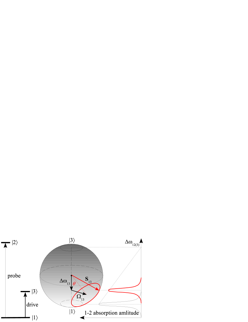
Figure 1: (Left) Three-level scheme and (right) effect of Rabi oscillations between the states $|1\rangle$ and $|3\rangle$ on the $|1\rangle-|2\rangle$ transition frequency and intensity. Here, for better visibility, the Rabi period $2\pi/\Omega_{13}$ is thought to be much longer than the time needed to detect the $|1\rangle-|2\rangle$ resonance line. The opposite case is considered in Secs. 3 and 4 below.

The situation in a three-level gas ($n_{3}\neq 0)$ is fundamentally different. We see that the interstate coherence of a spatially homogeneous gas can be probed by the contact shift in the presence the third state, like it has been done in fermionic ⁶Li Gupta . It is also remarkable that a homogeneous Fermi gas does exhibit a nonzero clock shift if the two states involved in the transition are not fully coherent with the third one ($C^{-}_{13}\neq 0$), the latter is populated ($n_{3}\neq 0$) and the respective scattering lengths are different ($a^{-}_{13}\neq a^{-}_{23}$). In this context, an incoherently populated third state acts as a buffer gas of foreign atoms. One can also see that, like in the case of just two levels, the coherence between the one-atom states $|1\rangle$ and $|2\rangle$ coupled by the resonance transition does not affect the clock shift $\Delta\omega_{12(3)}$ of this resonance.

In the absence of relaxation, the populations of the states $|1\rangle$ and $|3\rangle$ evolve (see Fig. 1) under continuous excitation of the transition $|1\rangle-|3\rangle$ in the initially $|1\rangle$-state sample as $n_{3}=n\sin^{2}\theta_{13}\sin^{2}\frac{\tilde{\Omega}_{13}t}{2}$, $n_{1}=n-n_{3}$, where $n$ is the total density of the gas, $\sin\theta_{13}=\Omega_{13}/\tilde{\Omega}_{13}$, $\tilde{\Omega}_{13}=\sqrt{\Delta\omega_{13}^{2}+\Omega_{13}^{2}}$, $\Omega_{13}$ is the respective Rabi frequency, and $\Delta\omega_{13}=\omega_{\rm d}-\omega_{13}$ is the detuning between the resonance frequency $\omega_{13}$ and the frequency $\omega_{\rm d}$ of the drive field. Note, that the gas remains fully coherent, since pseudo-spins $S_{13}$ of all atoms experience coherent precession on the $|1\rangle-|3\rangle$ Bloch sphere around the tilting angle $\theta_{13}$ and stay parallel to each other (Fig. 1). Thus, the resonance frequency $\omega_{13}$ remains unchanged while the $|1\rangle-|2\rangle$ transition is dynamically shifted to the frequency Saf_JLTP

$$\hbar\omega_{12}=\hbar\omega_{12}^{(0)}+2n\Delta\lambda\sin^{2}\theta_{13}\sin^{2}\frac{\tilde{\Omega}_{13}t}{2},$$ (3)

where $\Delta\lambda=\lambda^{+}_{23}-\lambda^{+}_{13}$. The amplitude of this frequency modulation can easily be comparable with or even much greater than the linewidth of the probe transition. Thus, excitation of the transition $|1\rangle-|3\rangle$ periodically drives the probe transition out of resonance. For clarity, Fig. 1 corresponds to slow driving in a sense that the Rabi period $2\pi/\Omega_{13}$ of the drive transition is thought to be much longer than the time needed to detect the $|1\rangle-|2\rangle$ resonance line. The opposite case of fast driving is considered in Secs. 3 and 4 below. At slow driving, the entire $|1\rangle-|2\rangle$ spectrum moves periodically fore and back along the frequency axis and simultaneously changes in amplitude. The waveforms shown in Fig. 1 are simply the snapshots of the spectrum at different phases of the Rabi cycle. Obviously, electromagnetic absorption at the fixed frequency $\omega_{\rm p}$ of the probe field also changes periodically with a period of the $|1\rangle-|3\rangle$ Rabi oscillations. It should be emphasized that these changes are associated with changes in both the population of the initial state and the transition frequency, in contrast to conventional double resonance, which is solely due to a change in the population of the initial state caused by the drive transitions. Clearly, such interaction-induced frequency modulation can greatly enhance the effect, which therefore can be called INteraction-Enhanced DOuble Resonance (INEDOR).

3 INEDOR spectrum

Let us consider in more detail a possible line shape of the INEDOR spectrum. In contrast to the case of slow driving illustrated in Fig. 1, we assume that simultaneous frequency and amplitude modulation of the $|1\rangle-|2\rangle$ absorption line is relatively fast (which is the case in a sufficiently high drive field) and therefore integrated by the detection system. This implies that the $|1\rangle-|3\rangle$ Rabi frequency is much higher than the rate of field or frequency sweep through the $|1\rangle-|2\rangle$ resonance or the inverse time constant $\tau^{-1}$ of the detection system, $\Omega_{13}\tau\gg 1$. In practice, as discussed in Sec. 4 below, a less severe condition $\tilde{\Omega}_{13}\tau\gg 1$ is sufficient. Thus, we deal with time-average absorption at the probe frequency in a sense that the absorption signal is integrated over many modulation (Rabi) cycles.

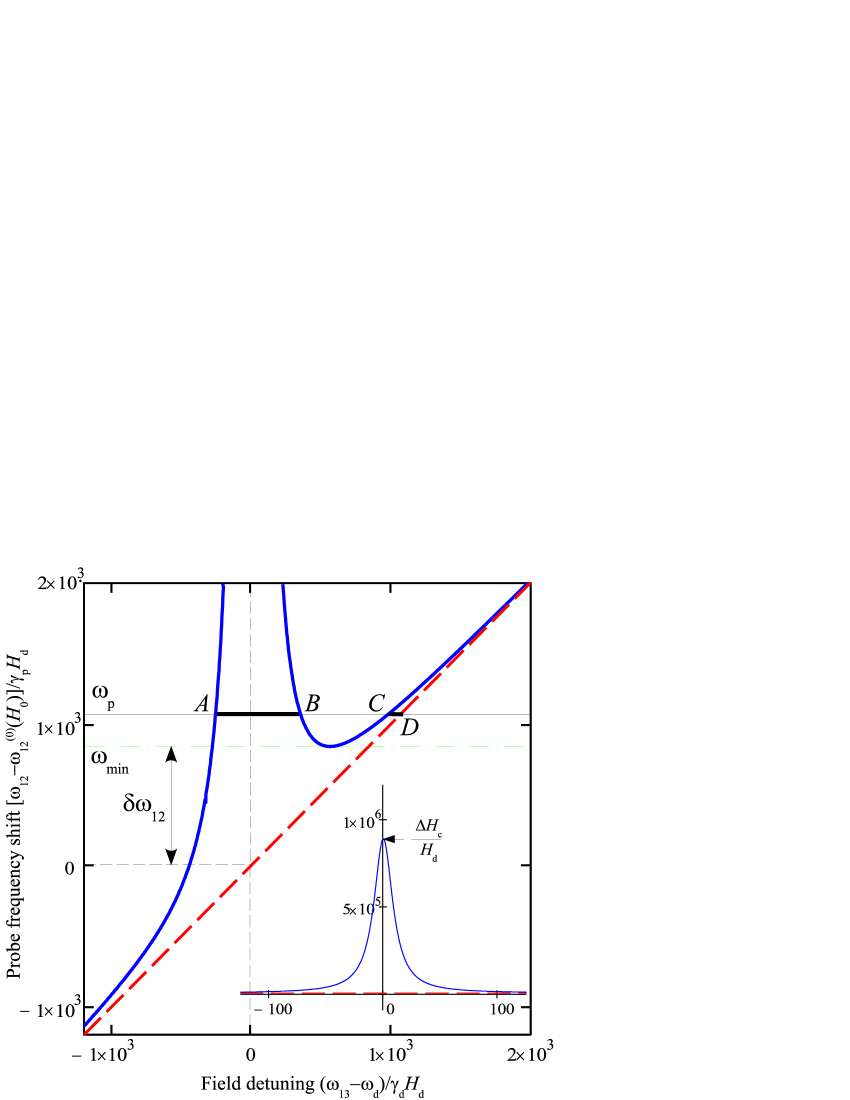
Figure 2: Field dependence of the $|1\rangle-|2\rangle$ frequency shift (in units of $\gamma_{\rm p}H_{\rm d}$) under the CW excitation of the $|1\rangle-|3\rangle$ resonance. Horizontal axis is the field detuning $(\omega_{13}-\omega_{\rm d})/\gamma_{\rm d}$ from the $|1\rangle-|3\rangle$ resonance in units of the excitation field $H_{\rm d}$. Solid and dashed line are, respectively, the upper bound of the sum of the Zeeman and mean-field contributions and the Zeeman contribution alone. Horizontal lines indicate (dash-dotted line) the value of $\omega_{12}$ at minimum and (solid line) the probe frequency. Vertical dashed line corresponds to the resonance field for the $|1\rangle-|3\rangle$ transition. The parameters correspond to 2D atomic hydrogen with a density of $3\cdot 10^{12}$ cm^-2 in a high polarizing field of 45 kG, except for the sign of the contact shift: $H_{\rm d}=1$ mG, $\Delta H_{\rm c}=89$ G, $\gamma_{\rm p}=\gamma_{e}$, $\gamma_{\rm d}=\gamma_{p}$. Inset is the overview of the same dependence.

Generally, the energies of all three levels and, consequently, both transition frequencies depend on the external static field. The nature of this field is insignificant but for definiteness we shall consider the magnetic field $H$. Since our analysis is conducted in terms of pseudo-spins, the respective contribution to the frequencies is the Zeeman splitting $\gamma_{\rm d(p)}H$, where $\gamma_{\rm d(p)}$ is the effective gyromagnetic ratio of the drive (probe) transition. Let the field $H_{0}$ correspond to the exact $|1\rangle-|3\rangle$ resonance, $\omega_{13}(H_{0})=\omega_{\rm d}$. Then the deviation $h=H-H_{0}$ of the field from this value results in the drive frequency detuning $\Delta\omega_{13}(h)=\gamma_{\rm d}h$. Owing to this Zeeman contribution to the effective precession frequency $\tilde{\Omega}_{13}$, the amplitude of the oscillating component of $\omega_{12}$ in Eq. (12), i.e., the amplitude of the frequency modulation of the probe transition turns out be a Lorentzian function of the field

$$\Delta\omega_{12}(h)=\left(\frac{2n\Delta\lambda}{\hbar}\right)\frac{H_{\rm d}^{2}}{H_{\rm d}^{2}+h^{2}},$$ (4)

where $H_{\rm d}$ is the amplitude of the drive field $H_{\rm d}(t)=H_{\rm d}\exp(i\omega_{\rm d}t)$, $\Omega_{13}=\gamma_{\rm d}H_{\rm d}$. On the other hand, the static (zero-density) component of $\omega_{12}$ also includes the Zeeman term

$$\omega_{12}^{(0)}(H_{0}+h)=\omega_{12}^{(0)}(H_{0})+\gamma_{\rm p}h.$$ (5)

The sum of these two contributions is an upper bound of the probe frequency,

$$\omega_{12}=\omega_{12}^{(0)}(H_{0})+\gamma_{\rm p}h+\left(\frac{2n\Delta\lambda}{\hbar}\right)\frac{H_{\rm d}^{2}}{H_{\rm d}^{2}+h^{2}}.$$ (6)

As a result, $\omega_{12}(t)$ oscillates between the Zeeman-only lower bound (Eq. (5), dashed line in Fig. (2)) and the Zeeman plus mean-field upper bound (Eq. (6), thick solid line in Fig. (2)) at the field-dependent frequency $\tilde{\Omega}_{13}(h)=\gamma_{\rm d}\sqrt{H_{\rm d}^{2}+h^{2}}$. As is seen from Eq. (6), the upper bound of the probe frequency is generally a nonmonotonic function of the static field.

As mentioned above, the Rabi frequency $\Omega_{13}=\tilde{\Omega}_{13}(0)$ is assumed to be sufficiently high, $\Omega_{13}\tau\gg 1$, in which case the absorption amplitude is integrated by the detection system over many Rabi cycles. The time-average absorption amplitude $A(h,\omega_{\rm p})$ within the bounds (5) and (6) is proportional to the average population of the initial state multiplied by the probability density $\rho(h,\omega_{\rm p})=[\tilde{\Omega}_{13}(h)/2\pi][d\omega_{12}(h,\omega_{\rm p})/dt]^{-1}$ to find the system at given $h$ and $\omega_{\rm p}$. It is readily shown that

$$A(h,\omega_{\rm p})\propto\frac{1-x}{2\pi\sqrt{x(\sin^{2}\theta_{13}(h)-x)}},$$ (7)

where

$$x=\frac{\hbar[\omega_{\rm p}-\omega_{12}^{(0)}(H_{0}+h)]}{2n\Delta\lambda}$$

and $1-x$ are the relative populations of the states $|3\rangle$ and $|1\rangle$, respectively. Thus, the probability density peaks at the lower ($x=0$) and upper ($x=\sin^{2}\theta_{13}(h)$) bound of the probe frequency. Note, that in the latter case absorption is further reduced due to a smaller population of the initial state and vanishes at $x=1$ (which implies $h=0$), i.e., at the maximum of the Lorentzian function (4).

The spectrum that appears when both the drive and probe frequency are fixed and the field is slowly swept through the resonance consists of up to four peaks corresponding to the field values, at which the probe frequency shown by the solid horizontal line in Fig. 2 crosses the upper (Zeeman plus mean-field) and lower (Zeeman only) bound of $\omega_{12}$ (points $A$, $B$, $C$, and $D$). The actual number of lines depends on the amplitude of the contact shift, the ratio $\gamma_{\rm d}/\gamma_{\rm p}$ of the Zeeman quanta of the excitation fields and the relation between the drive and probe frequency. The peaks lying within the drive resonance (i.e., within the segment $AB$ in Fig. 2) are much weaker because the atoms spend only a small fraction of time in the resonance conditions. This implies that the $|1\rangle-|2\rangle$ absorption amplitude is strongly decreased, which produces a “hole” in the resonance curve.

So far we considered a spatially homogeneous system. There could be three types of inhomogeneity associated with the inhomogeneous (i) static field, (ii) excitation fields and (iii) gas density. In terms of the upper bound of the probe frequency shift in Fig. 2, these correspond to a spread in (i) the overall vertical position of the curve (equivalent to the inhomogeneity of the probe frequency), (ii) the width of the drive resonance and (iii) the amplitude of the drive resonance plus the overall vertical shift.

To illustrate the effect of inhomogeneity we consider in more detail a linear gradient $\nabla H$ of the static field in an otherwise spatially homogeneous infinite sample. In this case, all possible field values are simultaneously present in different parts of the sample. Thus, the absorption amplitude at a given probe frequency $\omega_{\rm p}$ is proportional to the integral $I(\omega_{\rm p})=\int A(h,\omega_{\rm p})\left(\frac{\partial N}{\partial h}\right)dh$ of Eq. (7) along the $\omega_{\rm p}={\rm const}$ line within the bounds of the probe frequency (i.e., over the horizontal segments $AB$ and $CD$ in Fig. 2). Owing to a constant field gradient, integration over the field is equivalent to integration over space provided that the number of particles per unit volume $n$ is replaced by the number of particles per unit field $\frac{\partial N}{\partial h}\propto n|\nabla H|^{-1}$. The result of numerical integration with the parameters of experiments with 2D atomic hydrogen Ahokas ; Ahokas_JLTP ; Vas_priv is shown in Fig. 3 as a function of the drive frequency $\omega_{\rm d}$ (lower horizontal axis) at constant $\omega_{\rm p}$. Alternatively, the INEDOR spectrum can be detected by sweeping $\omega_{\rm p}$ (upper horizontal axis) at constant $\omega_{\rm d}$. In the latter case, the spectrum is inverted on the frequency scale because an increase in $\omega_{\rm d}$ corresponds to an increase in the resonance field $\omega_{\rm d}/\gamma_{\rm d}$ and, consequently, to a positive displacement of the mean-field Lorentzian peak on the $\omega_{12}(h)$ curve (6) in Fig. 2. The latter is equivalent to a negative change in the probe frequency $\omega_{\rm p}$ at constant $\omega_{\rm d}$. Which way of observing the INEDOR spectrum is preferred depends on the details of a particular experiment.

The absorption amplitude as a function of $\omega_{\rm d}$ (Fig. 3) is nearly constant well below and above the drive resonance, decreases substantially within the resonance and has a sharp maximum at $\omega_{\rm p}=\omega_{\rm min}$, i.e., when the minimum value of Eq. (6) coincides with the probe frequency. This explains the dispersion-looking ENDOR spectra of 2D atomic hydrogen Ahokas ; Ahokas_JLTP (see Sec.4 below). Physically, the hole in the absorption amplitude is because the atoms of the otherwise resonant region of the sample are dynamically driven out of the probe resonance and spend only a small fraction of time in the resonance conditions. As already mentioned, the probability of finding them in resonance peaks at the lower (5) and upper (6) bound of the probe frequency and, according to Eq. (7), is the lower the higher is the difference (4) between the two bounds of $\omega_{12}$. In this respect, there is no surprise that the positions of the $I$ minimum and the contact shift (4) maximum nearly coincide, $\omega_{\rm p}\approx\omega^{(0)}_{12}(H_{0})$. On the other hand, the absorption maximum is due to the fact that the drive resonance introduces zero gradient of the $|1\rangle-|2\rangle$ transition frequency in a certain region of the sample. As a result, much more atoms become resonant. A decrease in the population of the initial state $|1\rangle$ at the point of zero gradient turns out to be of minor importance for the chosen values of the parameters. However, according to Eq. (6), it can be significant at $|2n\Delta\lambda|\sim\hbar\gamma_{\rm p}H_{\rm d}$, which occurs at low gas density $n$ and strong drive field $H_{\rm d}$.

The dispersion-looking INEDOR spectrum of a gas in a spatially inhomogeneous static field can be also qualitatively explained in a different way. In the case of a positive contact shift, the parts of the inhomogeneously broadened probe resonance line are shifted towards higher fields by the amount proportional to the local amplitude of drive resonance curve. The shift increases with an increase in field at the low-field side of the drive resonance and decreases at its high-field side. Thus, the low-field side of the spectrum is “rarefied” whereas the high-field side is “compressed” in a sense that the number of atoms per unit field, which are involved in the probe transitions at lower (higher) fields, becomes smaller (larger). Accordingly, the probe absorption intensity is decreased at the low-field side of the drive resonance and increased at its high-field side. When $\omega_{\rm d}$ is swept from below at constant $\omega_{\rm p}$, the high-field side of drive resonance comes first. That is, the probe absorption intensity is increased at lower and decreased at higher $\omega_{\rm d}$, as illustrated by Fig. 3.

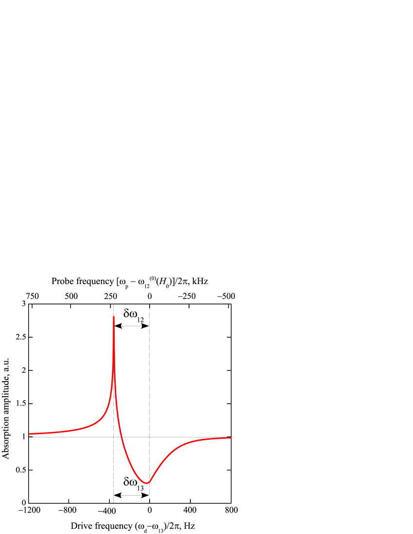
Figure 3: $|1\rangle-|2\rangle$ absorption amplitude as a function of drive frequency (expressed as the detuning, in Hertz, from the $|1\rangle-|3\rangle$ resonance) for the delta-functional spectrum of the probe field. Sharp peak corresponds to the frequency minimum in Fig. 2. Parameters are the same as in Fig. 2.

As discussed above, the width of the double-resonance curve in the probe-frequency units can be estimated as the difference $\omega_{\rm min}-\omega^{(0)}_{12}(H_{0})$ (see Fig. 2). For $|2n\Delta\lambda|\gg\hbar\gamma_{\rm p}H_{\rm d}$ the minimum of the right-hand side of Eq. (6) occurs at

$$\frac{(H^{2}_{\rm d}+h^{2})^{2}}{H^{2}_{\rm d}h}=\frac{4n\Delta\lambda}{\hbar\gamma_{\rm p}}.$$ (8)

Typically, $h\gg H_{\rm d}$ and Eq. (8) yields

$$h^{3}\simeq\frac{4n\Delta\lambda H^{2}_{\rm d}}{\hbar\gamma_{\rm p}}.$$ (9)

This corresponds to

$$\delta\omega_{12}\equiv\omega_{12}(h)-\omega^{(0)}_{12}(H_{0})\simeq\frac{3}{2}\gamma_{\rm p}h$$ (10)

and we finally arrive at

$$\delta\omega_{13}=\frac{\gamma_{\rm d}}{\gamma_{\rm p}}\delta\omega_{12}\simeq\frac{3}{2}\gamma_{\rm d}(2\Delta H_{\rm c}H^{2}_{\rm d})^{1/3},$$ (11)

where $\Delta H_{\rm c}=2n\Delta\lambda(\hbar\gamma_{\rm p})^{-1}$ is the maximum contact shift of the $|1\rangle-|2\rangle$ resonance in field units. Note, that the resonance linewidth depends on the gas density and drive field as $n^{1/3}H_{\rm d}^{2/3}$. Remarkably, the width of the INEDOR spectrum is independent of the static field gradient. On the other hand, the spectrum intensity is inversely proportional to $|\nabla H|$. A one-dimensional inhomogeneity of the drive field in the direction of $|\nabla H|$ also does not affect the linewidth because in this case $H_{\rm d}$ is a single-valued function of $h$. The effect of such an inhomogeneity is that the mean-field peak (4) becomes asymmetric and the INEDOR linewidth is determined by the local $H_{\rm d}$ value at the minimum of $\omega_{12}$ in Eq. (6). It is also worth mentioning that the linearity of the Zeeman contributions to $\omega_{12}$ and $\omega_{13}$ is unnecessary because these terms can be always linearized in the vicinity of the resonance field. In this case, the gyromagnetic ratios should be replaced by the respective field derivatives, $\gamma_{\rm d}\rightarrow\partial\omega_{13}/\partial H$ and $\gamma_{\rm p}\rightarrow\partial\omega_{12}/\partial H$.

4 ENDOR in atomic hydrogen

The spin states of a single hydrogen atom in a high magnetic field are commonly referred to as $|a\rangle\approx|-+\rangle$, $|b\rangle=|--\rangle$, $|c\rangle\approx|+-\rangle$, and $|d\rangle=|++\rangle$, in the order of increasing energy ($\pm$ signs stand for the projections of the electron and nuclear spin on the field direction; we also neglect small impurities of the opposite spin projections in the states $|a\rangle$ and $|c\rangle$). Ahokas et al. Ahokas ; Ahokas_JLTP observed a narrow feature in the ESR $|b\rangle-|c\rangle$ line while sweeping through the $|a\rangle-|b\rangle$ resonance. According to Eq. (1), the $|b\rangle-|c\rangle$ resonance is dynamically shifted to the frequency Saf_JLTP

$$\omega_{bc}=\omega_{bc0}+\frac{4\pi\hbar n}{ml}\Delta a\sin^{2}\theta_{ab}\sin^{2}\frac{\tilde{\Omega}_{ab}t}{2},$$ (12)

where $n$ is the 2D density of adsorbed H atoms and $l\sim 0.5$ nm is their out-of-plane delocalization length in the adsorption potential so that $n/l$ stands in place of the 3D density in Eqs. (1); $\Delta a=a_{s}-a_{t}=-30(10)$ pm Saf_JLTP ; Saf_Comment is the experimental difference between the singlet and triplet scattering length of two ground-state hydrogen atoms (to be compared with the theoretical values ranging from $-42$ to $-55$ pm Williams ; Jamieson ; Chakraborty ). The amplitude of the respective modulation of the resonance field in 2D atomic hydrogen at zero detuning ($\theta_{ab}=\frac{\pi}{2}$) is very large, $\Delta H_{\rm c}=1.5(5)\cdot 10^{-18}$ G$\cdot$cm³. At a typical 2D density of $3\cdot 10^{12}$ cm^-2, which corresponds to a 3D density of $6\cdot 10^{19}$ cm^-3, one has $\Delta H_{\rm c}\approx 90$ G. The amplitude of the drive RF field is $H_{\rm d}\sim 10^{-3}$ G Vas_priv and we find from Eqs. (12), (9) and (11) $h\sim 5.7\cdot 10^{-2}$ G and $\delta\omega_{ab}/2\pi\sim 350$ Hz, very close to a numerical result of 330 Hz for the maximum-to-minimum distance in Fig. 3. This agrees fairly well (and, remarkably, without any fitting parameters) with the 120-Hz experimental width of the ENDOR absorption signal reported in Ahokas ; Ahokas_JLTP . One should take into account that the contact shift in atomic hydrogen is negative and therefore the experimental spectrum is horizontally inverted with respect to the one shown in Fig. 3.

The experimental amplitude of the drive field corresponds to moderate Rabi frequency $\Omega_{13}\sim 30$ s^-1. However, the effective precession frequency $\tilde{\Omega}_{13}$ is two-three orders of magnitude higher in the most significant part of the spectrum ($h/H_{\rm d}\simeq 560)$ except for a very narrow region near zero detuning. On the other hand, the frequency was typically swept through the ENDOR line for $\tau\sim 1$ s Vas_priv . Thus, the condition $\tilde{\Omega}_{13}\tau\gg 1$ of fast driving was fulfilled. Note, that the experimental spectrum can be affected by inhomogeneity of the drive field and gas density across the 2D sample, as mentioned above. According to Eq. (9), both lead to inhomogeneity in the position of the sharp peak in Fig. 3, which is therefore substantially broadened and reduced in amplitude. Actually, in experiments Ahokas_JLTP , the amplitude of drive RF field was not exactly known and varied within the sample by a factor of three or so.

It can be shown that relaxation and other possible inelastic processes disregarded in the above consideration are of minor importance in atomic hydrogen Saf_JLTP . Neither should the spectral width $\delta\omega_{\rm p}/\omega_{\rm p}\sim 10^{-9}$ of the mm-wave source Ahokas_JLTP produce any noticeable effect, as it is much narrower than the INEDOR linewidth $\gamma_{\rm p}h/\omega_{\rm p}\sim 3\cdot 10^{-7}$ in probe-frequency units.

Ahokas et al. Ahokas ; Ahokas_JLTP also observed double resonance in a different way, by sweeping the static field at constant drive and probe frequencies and detecting the $|b\rangle-|c\rangle$ transition. This resulted in a change in the overall intensity of the absorption line depending on the drive frequency rather than in a narrow feature in the resonance curve, as one would expect from the above analysis. This issue remains unclear to us. Here, we can only mention that the case $\Omega_{13}^{2}\lesssim\gamma_{\rm d}|\partial H_{0}/\partial t|$ of slow driving or, equivalently, of fast sweeping, which could take place in such experiments, should be analyzed separately.

5 Conclusions

Thus, we have shown that simultaneous excitation of two transitions in a cold gas of multi-level atoms can result in nonlinear double resonance induced by a change in the contact shift of the probe transition frequency due to Rabi oscillations between the states involved in the drive transition. The linewidth of such interaction-enhanced double resonance is determined by the amplitude of the contact shift and the magnitude of the drive field and does not depend on the field gradient. The INEDOR line shape and width agree with those observed in 2D atomic hydrogen. Ahokas et al. Ahokas ; Ahokas_JLTP speculated that the double-resonance spectra they observed in atomic hydrogen could be due to electromagnetically-induced transparency or coherent population trapping, the well-known nonlinear effects in three-level systems. The detailed discussion of this opportunity will be presented elsewhere. Here, we have shown that there is at least another realistic scenario based on interaction-induced double resonance. In a way, it can be also regarded as electromagnetically-induced transparency, although the physical mechanisms behind these two coherent phenomena are totally different.

Reliable detection of conventional double resonance requires a significant (of order unity) depopulation of the initial state. As already explained in Sec. 1, INEDOR can be observed at a much lower depopulation because the probe transition frequency is driven completely out of resonance by even a very small population $n_{3}$ of the state $|3\rangle$. More specifically, the amplitude of the frequency modulation should be higher than the homogeneous linewidth of the probe transition or the spectral width of the source, whichever is greater. For example, in the case of 2D atomic hydrogen, the latter is $\delta\omega_{\rm p}/\omega_{\rm p}\sim 10^{-9}$ Ahokas_JLTP , which corresponds to $n_{3}\sim 2\cdot 10^{6}$ cm^-2 or $n_{3}/n\sim 10^{-6}$. Owing to such an ultimate sensitivity, the specific double resonance technique proposed in this work could be an effective tool for studying interactions in atomic systems and beyond.

References

- (1) S. Gupta et al., Science 300 (2003) 1723.
- (2) C. A. Regal and D. S. Jin, Phys. Rev. Lett. 90 (2003) 230404.
- (3) G. Baym, C. J. Pethick, Z. Yu, and M. W. Zwierlein, Phys. Rev. Lett. 99 (2007) 190407.
- (4) A. I. Safonov, I. I. Safonova and I. S. Yasnikov, J. Low Temp. Phys. 162 (2011)127.
- (5) G. K. Campbell et al., Science 324 (2009) 360.
- (6) K. Gibble, Phys. Rev. Lett. 103 (2009) 113202.
- (7) J. Ahokas, J. Järvinen and S. Vasiliev, Phys. Rev. Lett. 98 (2007) 043004.
- (8) J. Ahokas, J. Järvinen and S. Vasiliev, J. Low Temp. Phys. 150 (2007) 577.
- (9) B.D. Agap’ev, M.B. Gornyi, B.G. Matisov, Yu.V. Rozhdestvenskii, Sov. Phys. Uspekhi 36 (1993) 763.
- (10) A. I. Safonov, I. I. Safonova and I. I. Lukashevich, JETP Lett. 87 (2008) 23.
- (11) J. Ahokas, J. Järvinen, G. V. Shlyapnikov, and S. Vasiliev, Phys. Rev. Lett. 101 (2008) 263003.
- (12) D. M. Harber, H. J. Lewandowski, J. M. McGuirk and E. Cornell, Phys. Rev. A 66 (2002) 053616.
- (13) M. Zwierlein, Z. Hadzibabic, S. Gupta, and W. Ketterle, Phys. Rev. Lett. 91 (2003) 250404.
- (14) A. I. Safonov, I. I. Safonova and I. S. Yasnikov, Phys. Rev. Lett. 104 (2010) 099301.
- (15) C. J. Williams and P. S. Julienne, Phys. Rev. A 47, 1524 (1993).
- (16) M. J. Jamieson and B. Zygelman, Phys. Rev. A 64, 032703 (2001).
- (17) S. Chakraborty et al., Eur. Phys. J. D 45, 261 (2007).
- (18) S. Vasiliev, private communications (2011).