Substructure in the stellar halos of the Aquarius simulations

Abstract

We characterize substructure in the simulated stellar halos of Cooper et al. (2010) which were formed by the disruption of satellite galaxies within the cosmological N-body simulations of galactic halos of the Aquarius Project. These stellar halos exhibit a wealth of tidal features: broad overdensities and very narrow faint streams akin to those observed around the Milky Way. The substructures are distributed anisotropically on the sky, a characteristic that should become apparent in the next generation of photometric surveys. The normalized RMS of the density of stars on the sky appears to be systematically larger for our halos compared to the value estimated for the Milky Way from main sequence turn-off stars in the Sloan Digital Sky Survey. We show that this is likely to be due in part to contamination by faint QSOs and redder main sequence stars, and might suggest that $\sim 10\%$ of the Milky Way halo stars have formed in-situ.

1 Introduction

Stellar halos are repositories of merger debris and hence, despite their low luminosity, are central to efforts to unravel the accretion history of galaxies (Searle & Zinn, 1978). Wide-field photometric surveys have discovered a plethora of substructures in the halo of our Galaxy (e.g. Majewski et al., 2003; Belokurov et al., 2006; Jurić et al., 2008). Some examples are the Orphan Stream (Belokurov et al., 2007a) and the Sagittarius dwarf (Ibata et al., 1994) and its extended tidal tails (Ivezić et al., 2000; Yanny et al., 2000). Other conspicuous structures, like the Hercules-Aquila cloud (Belokurov et al., 2007b), the Virgo overdensity and the Virgo Stellar Structure, do not have the elongated appearance typical of tidal features and hence their nature is less obvious. Moreover, some of these structures strongly overlap on the sky but their relationship is not always clear (Martínez-Delgado et al., 2007; Duffau et al., 2006; Newberg et al., 2007).

The amount of spatial substructure present in the outer halo has been quantified by Bell et al. (2008, see also de Jong et al. 2010). These authors found RMS fluctuations of order 30–40% with respect to a smooth halo model. Taken at face value, this implies that at least this fraction of the stellar halo has been accreted. Starkenburg et al. (2009) determined that at least 10% of the outer halo must have been accreted, based on the amount of clustering present in the Spaghetti Survey (which also included radial velocity information). Roughly half of this survey’s pencil beams pointed to portions of the sky unexplored by SDSS; intriguingly, these authors found no evidence of substructure in those regions, suggesting that the distribution of outer halo substructure may be very anisotropic.

Several studies have examined the properties of stellar halos in $\Lambda$CDM simulations of structure formation. For example, Bullock & Johnston (2005) followed the accretion of satellites onto a smooth, time-dependent gravitational potential resembling a Milky Way galaxy. Their simulations produce very lumpy stellar halos, with extended tidal streams covering large portions of the sky. De Lucia & Helmi (2008) used high-resolution cosmological N-body simulations of the formation of a Milky-Way size dark halo in combination with a semi-analytic model of galaxy formation. Although their model reproduces the global properties of the Galactic stellar halo, the resolution of the simulations was too low to show much substructure in the form of tidal tails.

Recently, Cooper et al. (2010, hereafter C10) have combined full cosmological dark matter simulations from the Aquarius project with the Durham semi-analytic galaxy formation model, galform, in order to follow the assembly of ‘accreted’ stellar halos. The extremely high resolution of the Aquarius halos permits a wealth of substructure to be studied in the Cooper et al. models. This Letter will focus on the properties of this substructure as may be revealed by ongoing (e.g. SDSS) and future wide-field photometric surveys, such as Skymapper, Pan-STARRS or LSST.

2 Brief description of the model

The Aquarius project consists of simulations of the formation of several dark matter halos with masses comparable to that of the Milky Way in a $\Lambda$CDM universe. The Aquarius halos (labelled Aq-A to Aq-E) are resolved with more than $10^{8}$ particles, and their properties are described in Springel et al. (2008). To follow the evolution of the baryonic component, the dynamical information obtained from the simulations is coupled to the Durham semi-analytic galaxy formation model (Bower et al., 2006). In essence, C10 identify at each output the halos that host galaxies according to the semi-analytic model, and tag the 1% most bound particles at that time with “stellar properties” such as masses, luminosities, ages and metallicities. This allows us to follow the assembly and dynamics of the accreted component of galaxies.

Note, however, that we do not follow stellar populations formed in-situ (for example, a disc component) because our dynamical simulations are purely collisionless (hydrodynamics and star formation are treated semi-analytically). A massive disc may influence satellite orbits and their debris, and also provide a reservoir from which stars can be scattered into the halo, but these effects are absent in our models.

The tagging scheme leads to the identification of more than $4\times 10^{5}$ tracer dark matter particles for Aq-A and up to a maximum of $6\times 10^{5}$ for Aq-B and Aq-D. Since the stellar mass assigned to each of these dark matter particles depends on the mass of stars formed in the parent galaxy with time, they do not all carry the same weight (for more details, see C10). Therefore, and for ease of comparison to observations, we have resampled the tagged particles as follows. For each tagged dark matter particle we find the 32 neighbors ranked as nearest simultaneously in position and in velocity at the present time amongst the class of tagged particles that share the same progenitor. We then measure the principal axes of the spatial distribution of these neighboring particles. This is used to define the characteristics of a multivariate Gaussian from which we draw positions for re-sampled stars. We then down-sample this new set of “stellar particles” to represent main sequence turn-off stars (assuming $5\,{\rm M}_{\odot}$ per MSTO, as used in Bell et al., 2008) or red giant branch stars (we assume 1 RGB per 8 MSTO stars, as in the models of Marigo et al., 2008). This results in $\sim 5.5\times 10^{7}$ MSTO stars between 1 kpc and 50 kpc from the halo center for Aq-A, and up to $\sim 1.83\times 10^{8}$ MSTO stars for Aq-D (which is the brightest of our stellar halos).

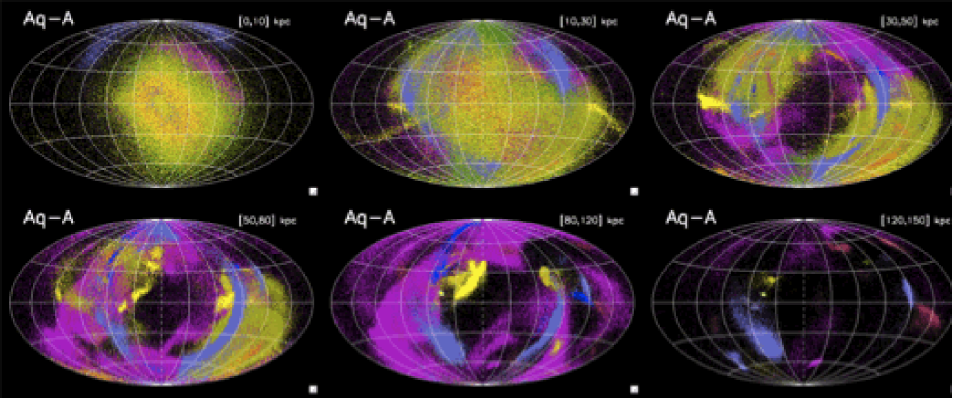
Figure 1: Distribution of “field” RGB stars on the sky at various distances from the “Sun” for the stellar halo of Aq-A. The different colors correspond to stars originating in different progenitors. The total number of progenitors is 163, out of which 53 contribute more than $10^{4}\,{\rm M}_{\odot}$ in stars. There are 35 different progenitors contributing at least 50 RGB stars in the innermost bin, and 48 at distances between 10 and 30 kpc. This number drops down to 10 in the most distant bin considered here. Thus the Aq-A stellar halo is most diverse between 10 and 30 kpc.

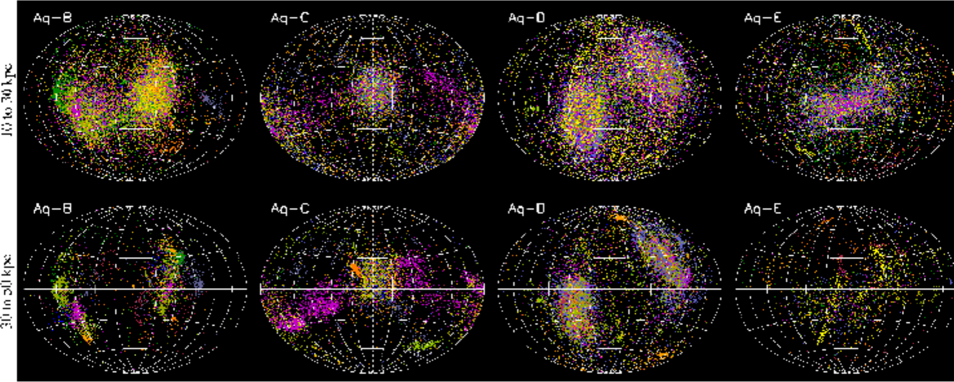
Figure 2: Sky distribution of RGB stars located at “heliocentric” distances [10, 30] kpc (top) and [30,50] kpc (bottom) for the set of Aquarius stellar halos.

3 Results

In this Letter we focus on the distribution of halo stars on the sky for direct comparison to photometric surveys. We will show that panoramic views resembling the “Field of Streams” are common in our simulations, and we will provide a new theoretical perspective on the nature of the overdensities discovered by SDSS. At the end, we quantify the amount of substructure present in our stellar halos and compare it to the results of Bell et al. (2008). In future papers we will focus on the characterization of substructure (width, age, relation to progenitor system, etc.), and on the amount of kinematic substructure present in the Solar neighborhood (especially for comparison with RAVE, and Gaia data in the future; Gómez et al. in prep.).

3.1 Distribution on the sky

Figure 1 shows the distribution in the sky of the RGB stars present in the stellar halo of Aq-A. The different panels in Fig. 1 correspond to stars located at increasing distance from the Sun, which is assumed to be at (-8, 0, 0) kpc with respect to the halo center (for this strongly prolate halo, the major axis is very nearly aligned with the $z$-axis of the simulation reference frame). Particles that have the same color represent stars formed in the same parent galaxy.

This figure shows that the distribution of stars in the accreted halo is very smooth in the inner 10 kpc. Substructure becomes apparent at $\sim 20$ kpc and dominates the halo beyond $\sim$30 kpc. The substructures are often diffuse, particularly at small distances from the galactic center. This is because their progenitor satellites are relatively massive. For example, the most prominent streams in Fig. 1 are those in magenta (visible at all distances), green (dominant in the very center), blue-gray (which we describe below as a Sgr analogue) and light green (prominent beyond 30 kpc). These contribute $1.3\times 10^{8}$, $1.4\times 10^{8}$, $2.2\times 10^{7}$ and $4.5\times 10^{7}$ M_⊙ respectively, i.e. all together they add up to 85% of the stellar mass in the halo of Aq-A.

The distribution of substructure on the sky is anisotropic, and appears to be preferentially found along a “ring”. In this region, a system of streams very similar to those of the Sagittarius dwarf galaxy is apparent (shown in blue-gray). Even the central regions of the stellar halo of Aq-A are not isotropic on the sky – a bar-like feature is visible towards the galactic center. The central region of this stellar halo is triaxial, which may also be true in the case of the Milky Way (Newberg et al., 2007). However, it is likely that the degree of triaxiality would decrease if a massive stellar disk were included in the simulation (see e.g. Dubinski, 1994; Debattista et al., 2008; Kazantzidis et al., 2004, 2010; Tissera et al., 2009).

Figure 2 shows the sky distribution of stars located between 10 and 30 kpc (top) and 30 to 50 kpc (bottom) for the remaining halos. Substructure is apparent in all cases, but there are large variations in its coherence, surface brightness and distribution across the sky. As in the case of Aq-A , the most significant overdensities are found at 10 - 30 kpc, although abundant substructure is also present at larger distances.

The object found in Aq-A that resembles Sagittarius and its streams became a satellite at redshift 1.74 (9.7 Gyr ago), and had a total mass of $2.9\times 10^{10}\,{\rm M}_{\odot}$ and a stellar mass of $2.7\times 10^{7}\,{\rm M}_{\odot}$ at the time of infall. A bound core survived until the present day with approximately 25% of the initial stellar mass. Fig. 3 shows that its streams cover a similar area of the sky and have distances comparable to those of the Sagittarius streams in the Milky Way halo.

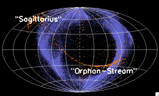
Figure 3: Sky distribution of RGB stars in Aq-A from the “Sagittarius” (blue) and “Orphan” (orange) streams analogues. Only those stars located at distances smaller than 80 kpc from the “Sun” are shown.

We also find structures that resemble the Orphan stream. Although they are not common at small radii, very low surface brightness thin streams are present, and can be found as close as 10 kpc from the halo center. Typically they have elongated orbits, and their characteristic apocentric distances range from 30 kpc up to $\sim 130$ kpc. This explains why they have remained coherent despite the triaxial shape of the halo (and the graininess of the potential). Such streams originate in low mass galaxies. For example, the progenitor of the thin stream shown in Fig. 3 had a total mass of $1.2\times 10^{8}\,{\rm M}_{\odot}$, a stellar mass of $10^{5}\,{\rm M}_{\odot}$ and was accreted into Aq-A at $z=5$, i.e. $\sim 12.5$ Gyr ago.

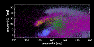
Figure 4: Distribution of MSTO stars in the Aquarius “Field of Streams” colored according to provenance. The region of the sky shown here has a similar extent to the SDSS footprint, but the model “stars” are located in a thin slice of 1 kpc width at a distance of $\sim 35$ kpc. Streams from different progenitors overlap on the sky because of the correlated infall directions and also due to group infall (both characteristic of $\Lambda$CDM). This constitutes a plausible (alternative) explanation of the observed bifurcation of the Sgr stream.

3.2 The “Field of Streams”

The previous figures show that in our simulations, streams from different progenitors frequently overlap on the sky. This is due mostly to the correlated infall pattern of the progenitor satellites from which these streams originate. For example, Aq-A remains embedded in the same large-scale coherent filament for $\sim 10$ Gyr before the present day, and many of its satellites have formed in this structure (cf Libeskind et al., 2005, also Lovell et al. 2010, Vera-Ciro et al. in prep.).

This is exemplified in Fig. 4, which plots the distribution of MSTO stars (generated following our simple prescription) for Aq-A in a thin distance slice through a region similar to the SDSS footprint known as the “Field of Streams” (Belokurov et al., 2006). Here different colors indicate different progenitor systems. The characteristics of this Aquarius “Field of Streams” are similar to those observed in SDSS. In particular, we see streams of stars that follow similar paths on the sky, resembling the bifurcation discovered by Fellhauer et al. (2006), as well as various broad overdensities. Note that some of the bifurcations that are apparent do not necessarily arise from the overlap of streams on the same orbit with different orbital phase, but instead correspond to the overlap of streams of different origin. This implies that measurements of position and distance alone may be insufficient to associate overdensities in nearby regions of the sky with a single parent object; therefore some caution is required when such associations are used to constrain the shape of the underlying gravitational potential.

3.3 Quantifying the amount of substructure

Following Bell et al. (2008), we have selected stars from SDSS-DR7 with $140^{\rm o}\leq\alpha\leq 220^{\rm o}$ and $0^{\rm o}\leq\delta\leq 60^{\rm o}$, $0.2<(g$–$r)<0.4$ (characteristic of the halo MSTO), and with apparent magnitude $18.5\leq r\leq 22.5$. If an absolute magnitude $M_{r}\sim 4.5$ is assumed, these stars would probe a distance range of 7 up to 35 kpc. In practice, this simple ‘tomography’ of the halo is subject to various uncertainties.

For example, using data from SDSS Stripe 82, Jurić et al. (2008) estimated that at the bright end, 5% of the point-like sources with $0.2<(g$–$r)<0.3$ are QSOs. At $r\sim 22$, this fraction increases to 34%, which extrapolated to $r\sim 22.5$, implies a non-negligible contamination of 50%. Another complication arises from photometric errors. Although these are relatively small, the color error at the faint end is $\sigma_{g-r}\sim 0.2$, i.e. comparable to the width of the MSTO color selection box (Ivezić et al., 2008). Therefore, a large number of lower main sequence stars are scattered into the MSTO region, leading to an incorrect assignment of absolute magnitudes. We consider both of these effects in our simulations.

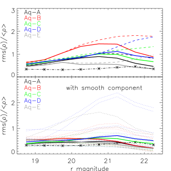
Figure 5: RMS to mean density of MSTO “stars” in a region of the sky similar in location and extent to the SDSS footprint as a function of apparent magnitude for our accreted Aq-halos. Top panel: The dashed curves indicate the raw measurements, while the solid curves take into account photometric errors and QSO contamination. Bottom panel: A smooth component with 10% of the total stellar halo mass has been added to each Aq-halo. The measurements for eight observers located along the “solar” circle are given by the dotted curves, while their median value is shown in solid. In both panels, the black asterisks correspond to the values estimated from SDSS data for the Milky Way.

We measure the RMS in the sky density of sources identified as halo MSTO stars in the SDSS as a function of apparent magnitude, in cells of 2$\times$2 deg². To compare with the simulations, we derive the apparent magnitude of each model MSTO stellar particle as $m_{r}=5\log d-5+M_{r}+\Delta M_{r}$. Here $d$ is the distance to the observer, and $M_{r}$ is a random variable following a Gaussian distribution with $\langle M_{r}\rangle=4.5$ and $\sigma=0.9$ (to mimic the spread in the absolute magnitude of the MSTO). The term $\Delta M_{r}$ accounts for the uncertainty due the color error $\sigma_{g-r}$, and is computed as $\Delta M_{r}={\rm d}M_{r}/{\rm d}(g-r)\times\sigma_{g-r}\times u$, where ${\rm d}M_{r}/{\rm d}(g-r)$ is the slope of the main sequence track (derived from the photometric parallax relations by Jurić et al., 2008), and $u$ is a normally distributed random variable with zero mean and unity dispersion.

In our simulations, we place eight observers along a circle of 8 kpc radius from the halo center, in a plane perpendicular to the minor axis of the dark matter halo (an approximation to the Solar circle). We select those MSTO “stars” located in the same region of the sky and with the same apparent magnitude range as the SDSS sample, and we measure the (Poisson-corrected) RMS in the projected surface density of these stars for each of our halos. Finally, we add the expected contamination by QSOs as described above. In this way, we obtain the fractional RMS which may be compared to the measurement from SDSS.

In the top panel of Fig. 5 the solid curves denote the median (of each of the 8 independent observers) for each halo. The dashed curves correspond to the raw RMS obtained without taking into account the effect of photometric errors and QSO contamination. This figure shows that our halos tend to have systematically larger fractional RMS values than found in the SDSS data. The bottom panel of Fig. 5 shows the RMS statistic when we include the contribution of a smooth component. We plot both the median RMS for each halo (solid) as well as that measured by each of the 8 observers (dotted). Here we have assumed 10% of the total stellar halo mass to be distributed following a Hernquist profile with scale radius of 1.25 kpc, although our results are not strongly dependent on the exact value of this parameter (note that at $r\sim 19$, its contribution is $\sim 30$%). This component would represent stars formed in the Galaxy itself, which, by definition, are absent in the C10 models of accreted halos. The main effect is to lower the contrast between cells with and without overdensities. The comparison to the SDSS results improves noticeably, indicating that there is indeed room for an in-situ component to be present in the stellar halo of the Milky Way (see also Zolotov et al., 2009).

4 Summary

We have discussed the substructure present in the stellar halos of Cooper et al. (2010) which were formed by the disruption of accreted satellites within the Milky Way mass $\Lambda$CDM halos of the Aquarius project. Diffuse features such as the Pisces and Virgo overdensities and the Hercules-Aquila cloud are relatively common, as are narrow, faint “orphan” streams. One of our halos even contains a structure similar to the Sagittarius Stream. We have found that substructures are not distributed isotropically on the sky. This is likely to be related to the correlated infall of satellites accreted along large-scale filaments, a characteristic feature of the cold dark matter model (Libeskind et al., 2005; Li & Helmi, 2008; Lux et al., 2010). As a consequence, chance alignments between streams from different progenitors may occur (as in our “Sagittarius” example), which may be easily misinterpreted as streams from the same object with different orbital phase. We find that the fraction of substructure in our models is somewhat higher than is estimated for the Milky Way. The addition of a smooth spheroidal component that contains 10% of the total stellar halo mass is required to match the simulations the SDSS data. This might suggest that a fraction of the halo stars formed in-situ. However, the discrepancy could also, however, be the result of limitations in our modeling techniques or uncertainties in the interpretation of the SDSS data.

References

- Bell et al. (2008) Bell, E. F., et al. 2008, ApJ, 680, 295
- Belokurov et al. (2006) Belokurov, V., et al. 2006, ApJ, 642, L137
- Belokurov et al. (2007a) Belokurov, V., et al. 2007, ApJ, 658, 337
- Belokurov et al. (2007b) Belokurov, V., et al. 2007, ApJ, 657, L89
- Bower et al. (2006) Bower, R. G., Benson, A. J., Malbon, R., Helly, J. C., Frenk, C. S., Baugh, C. M., Cole, S., & Lacey, C. G. 2006, MNRAS, 370, 645
- Bullock & Johnston (2005) Bullock, J. S., & Johnston, K. V. 2005, ApJ, 635, 931
- Cooper et al. (2010) Cooper, A. P., et al. 2010, MNRAS, 406, 744
- Debattista et al. (2008) Debattista, V. P., Moore, B., Quinn, T., Kazantzidis, S., Maas, R., Mayer, L., Read, J., & Stadel, J. 2008, ApJ, 681, 1076
- de Jong et al. (2010) de Jong, J. T. A., Yanny, B., Rix, H.-W., Dolphin, A. E., Martin, N. F., & Beers, T. C. 2010, ApJ, 714, 663
- De Lucia & Helmi (2008) De Lucia, G., & Helmi, A. 2008, MNRAS, 391, 14
- Dubinski (1994) Dubinski, J. 1994, ApJ, 431, 617
- Duffau et al. (2006) Duffau, S., Zinn, R., Vivas, A. K., Carraro, G., Méndez, R. A., Winnick, R., & Gallart, C. 2006, ApJ, 636, L97
- Fellhauer et al. (2006) Fellhauer, M., et al. 2006, ApJ, 651, 167
- Helmi (2008) Helmi, A. 2008, A&A Rev., 15, 145
- Ibata et al. (1994) Ibata, R. A., Gilmore, G., & Irwin, M. J. 1994, Nature, 370, 194
- Ivezić et al. (2000) Ivezić, Ž., et al. 2000, AJ, 120, 963
- Ivezić et al. (2008) Ivezić, Ž., Tyson, J. A., Allsman, R., Andrew, J., Angel, R., & for the LSST Collaboration 2008, arXiv:0805.2366
- Jurić et al. (2008) Jurić, M., et al. 2008, ApJ, 673, 864
- Kazantzidis et al. (2004) Kazantzidis, S., Kravtsov, A. V., Zentner, A. R., Allgood, B., Nagai, D., & Moore, B. 2004, ApJ, 611, L73
- Kazantzidis et al. (2010) Kazantzidis, S., Abadi M. G. & Navarro J. F., 2010, ApJ, 720, L62
- Li & Helmi (2008) Li, Y.-S., & Helmi, A. 2008, MNRAS, 385, 1365
- Libeskind et al. (2005) Libeskind, N. I., Frenk, C. S., Cole, S., Helly, J. C., Jenkins, A., Navarro, J. F., & Power, C. 2005, MNRAS, 363, 146
- Lovell et al. (2010) Lovell, M., Eke, V., Frenk, C., & Jenkins, A. 2010, arXiv:1008.0484
- Lux et al. (2010) Lux, H., Read, J. I., & Lake, G. 2010, MNRAS, 406, 2312
- Majewski et al. (2003) Majewski, S. R., Skrutskie, M. F., Weinberg, M. D. & Ostheimer, J. C. 2003, ApJ, 599, 1082
- Marigo et al. (2008) Marigo, P., Girardi, L., Bressan, A., Groenewegen, M. A. T., Silva, L., & Granato, G. L. 2008, A&A, 482, 883
- Martínez-Delgado et al. (2007) Martínez-Delgado, D., Peñarrubia, J., Jurić, M., Alfaro, E. J., & Ivezić, Z. 2007, ApJ, 660, 1264
- Newberg et al. (2007) Newberg, H. J., Yanny, B., Cole, N., Beers, T. C., Re Fiorentin, P., Schneider, D. P., & Wilhelm, R. 2007, ApJ, 668, 221
- Robin et al. (2003) Robin, A. C., Reylé, C., Derrière, S., & Picaud, S. 2003, A&A, 409, 523
- Starkenburg et al. (2009) Starkenburg, E., et al. 2009, ApJ, 698, 567
- Searle & Zinn (1978) Searle, L., & Zinn, R. 1978, ApJ, 225, 357
- Springel et al. (2008) Springel, V., et al. 2008, MNRAS, 391, 1685
- Tissera et al. (2009) Tissera, P. B., White, S. D. M., Pedrosa, S., & Scannapieco, C. 2009, arXiv:0911.2316
- Yanny et al. (2000) Yanny, B., et al. 2000, ApJ, 540, 825
- Zolotov et al. (2009) Zolotov, A., Willman, B., Brooks, A. M., Governato, F., Brook, C. B., Hogg, D. W., Quinn, T., & Stinson, G. 2009, ApJ, 702, 1058