The three-dimensional Heisenberg spin glass under a weak random anisotropy.

Abstract

We perform a finite size scaling study of the three-dimensional Heisenberg spin glass in the presence of weak random anisotropic interactions, up to sizes $L=32$. Anisotropies have a major impact on the phase transition. The chiral-glass susceptibility does not diverge, due to a large anomalous dimension. It follows that the anisotropic spin-glass belongs to a Universality Class different from the isotropic model, which questions the applicability of the chirality scenario.

I INTRODUCTION

Spin glasses (SG’s) are disordered magnetic alloys, widely regarded as paradigmatic complex systems.SGINTRO The degree of anisotropy in the magnetic interactions determines whether a particular alloy is classified as a Heisenberg or an Ising SG (Ising corresponds to a limit of strong anisotropy). Experimentally, anisotropies affect significantly the glassy response to external magnetic fields and the behavior under cooling protocols.BERT04

Theorists have privileged the study of the Ising limit, in spite of the fact that canonical SG’s, e.g. CuMn or AgMn, should be rather regarded as Heisenberg, with weak anisotropic interactions. Indeed, complications arise in the Heisenberg case. In addition to the standard SG ordering, Heisenberg systems show as well a chiral-glass (CG) phase, where chiralities order VILLAIN (chiralities, also named vorticities, reflect the handedness of the non-collinear spin ordering pattern, see definitions below).

Probably motivated by failures in early numerical attempts Tc0 to find a standard SG phase for Heisenberg systems, Kawamura proposed a chirality scenario, expected to hold for most experimental systems.CHIRALSCEN_KAWAMURA In the ideal, fully isotropic case, the standard SG critical temperature $T_{\mathrm{SG}}$ would be strictly zero, while chiralities would order at $T_{\mathrm{CG}}>0$ (spin-chirality decoupling). Yet, anisotropic interactions (either dipolar, pseudo-dipolar or Dzyaloshinskii-MoriyaLEVYFERT ; BRAYMOORE ), albeit small, are unavoidable in experimental samples. Hence, the scenario includes a decoupling-recoupling hypothesis: weak random anisotropic interactions would recouple spins and chiralities so that $T_{\mathrm{CG}}=T_{\mathrm{SG}}>0$. Indeed, the numerical work available at the time indicated that very small amounts of anisotropy lead to $T_{\mathrm{SG}}>0$.MATSUBARA

CG ordering may be experimentally investigated through the anomalous Hall effect. Due to spin-orbit interaction and the spin polarization of the conduction electrons, the anomalous Hall resistivity picks contributions proportional to the CG order parameter and to its corresponding non-linear susceptibility.AHE_TAKA ; AHE_KAWA The effectiveness of this tool to study non-coplanar orderings has been demonstrated in manganites,AHE-MANG and in a geometrically frustrated pyrochlore ferromagnet.AHE-SC

The effect of anisotropies on the critical behavior was considered by Bray and Moore,BRAYMOORE before the question of chiral ordering was raised. They predicted that these systems belong to the Ising SG’s Universality Class, no matter the kind of anisotropic interactions. However, in their analysis the assumption was made that $T_{\mathrm{SG}}\!=\!0$ in the isotropic limit (this assumption seemed plausible at the time, although we now know that it is incorrect).

Recent theoretical work has shown that the chirality scenario needs some revision. New simulation algorithms (allowing to thermalize at lower temperatures than pioneering work Tc0 ), combined with modern finite-size scaling (FSS) methods,BALLESTEROS ; QUOTIENTS ; VICTORAMIT have provided conclusive evidence for a standard SG ordering with $T_{\mathrm{SG}}>0$ for purely isotropic interactions.LEEYOUNG ; LEEYOUNG2 ; HSGWE ; HSG-LVSAP ; VIET-KAWAMURA ; OTROS ; MATSHIENTA Only some controversy remains on whether $T_{\mathrm{SG}}$ is slightly smaller than $T_{\mathrm{CG}}$,VIET-KAWAMURA or rather the two are compatible within errors.HSG-LVSAP Interestingly enough, a modern-styled study seems to be still lacking for the more realistic case of a Heisenberg SG with small random anisotropy.

Here we show that small anisotropic interactions cause that, at variance with the ideal case, the CG susceptibility no longer diverges at $T_{\mathrm{CG}}$ (i.e. the anomalous dimension becomes $\eta_{\mathrm{CG}}>2$). In the Renormalization Group framework,VICTORAMIT anisotropy is a relevant perturbation. Even if in an experimental sample anisotropies are fairly small, the isotropic model is appropriate only for moderate correlation length. Closer to the critical temperature, a new fixed point rules (presumably in the Ising SG Universality Class, due to spin-reversal symmetry). A slow crossover VICTORAMIT from the Heisenberg to the anisotropic fixed-point arises upon approaching the phase transition. We conjecture that this crossover explains FN1 experimental claims of a non-trivial dependency of critical exponents on the anisotropy strength.BERT04 ; CAMPBELLPETIT Our results follow from a FSS analysis of equilibrium Monte Carlo simulations on system-sizes up to $L\!=\!32$. Data suggest that anisotropies cause a temperature range in which chiralities order while spins do not (i.e. $T_{\mathrm{SG}}<T_{\mathrm{CG}}$). However, due to the slow crossover, further research will be needed to dismiss spin-chirality recoupling.

The remaining part of this work is organized as follows. We define the model and describe our numerical methods in Sect. II. We address thermal equilibration, a major issue in any spin-glass simulation, in Sect. III. Our physical results are reported in Sect. IV. Finally, we give our results in Sect. V.

II MODEL AND SIMULATIONS

Since the main types of anisotropic interactions lead to the same effective replica Hamiltonian,BRAYMOORE it is numerically convenient to study short range (pseudo-dipolar) interactions. Take the Edwards-Anderson model on a cubic lattice of size $L$, with periodic boundary conditions. Heisenberg spins occupy the lattice nodes $\boldsymbol{x}$ [$\vec{S}_{\boldsymbol{x}}=(S_{\boldsymbol{x}}^{1},S_{\boldsymbol{x}}^{2},S_{\boldsymbol{x}}^{3})$, $\vec{S}_{\boldsymbol{x}}\cdot\vec{S}_{\boldsymbol{x}}=1\,$]. The Hamiltonian is MATSUBARA

$$H=-\sum_{\langle\boldsymbol{x},\boldsymbol{y}\rangle}\left(J_{\boldsymbol{x}\boldsymbol{y}}\vec{S}_{\boldsymbol{x}}\cdot\vec{S}_{\boldsymbol{y}}+\vec{S}_{\boldsymbol{x}}\cdot D_{\boldsymbol{x}\boldsymbol{y}}\vec{S}_{\boldsymbol{y}}\right),$$ (1)

($\langle\boldsymbol{x},\boldsymbol{y}\rangle$: lattice nearest-neighbors). The random exchange-couplings, $J_{\boldsymbol{x}\boldsymbol{y}}$, are Gaussian distributed with $\overline{J_{\boldsymbol{x},\boldsymbol{y}}}=0$, and $\overline{J^{2}_{\boldsymbol{x},\boldsymbol{y}}}=1$. The random $D_{\boldsymbol{x}\boldsymbol{y}}$ are $3\times 3$ symmetric matrices (i.e. $\vec{S}_{\boldsymbol{x}}\cdot D_{\boldsymbol{x}\boldsymbol{y}}\vec{S}_{\boldsymbol{y}}=D_{\boldsymbol{x}\boldsymbol{y}}\vec{S}_{\boldsymbol{x}}\cdot\vec{S}_{\boldsymbol{y}}$). Their matrix elements are independent and uniformly distributed in $(-D,D)$. In most of the work reported here $D=0.05$ (which corresponds to the best studied case MATSUBARA ), but we will be presenting results for $D=0.1$ as well.

The ideal limit of a fully isotropic Heisenberg model is recovered from Eq. (1) by setting $D=0$. Once $D>0$, the original $\mathrm{O(3)}$ symmetry, corresponding to a global spin rotation (or reflection), is lost. The only remaining symmetry for $D>0$ is global spin inversion.

An instance of the couplings, $\{J_{\boldsymbol{x},\boldsymbol{y}},D_{\boldsymbol{x},\boldsymbol{y}}^{\mu\nu}\}$ is named a sample. For any physical quantity, we first obtain the thermal average, denoted as $\langle\ldots\rangle$. Only afterwards we perform the sample average (denoted by an overline).

Defining the SG and CG susceptibilities requires real replicas. We consider pairs of spin configurations, $\vec{S}_{\boldsymbol{x}}^{a}$ and $\vec{S}_{\boldsymbol{x}}^{b}$, that evolve with independent thermal noise, under the same couplings and at the same temperature. The spin-overlap field is $q_{\boldsymbol{x}}=\vec{S}_{\boldsymbol{x}}^{a}\cdot\vec{S}_{\boldsymbol{x}}^{b}$, while its Fourier transform at wave vector $\boldsymbol{k}$, is $\hat{q}_{SG}(\boldsymbol{k})=\sum_{\boldsymbol{x}}q_{\boldsymbol{x}}~{}\mathrm{e}^{\mathrm{i}\boldsymbol{k}\cdot\boldsymbol{x}}/N$. On the other hand, the local chirality is defined as:

$$\zeta_{\boldsymbol{x}\mu}=\vec{S}_{\boldsymbol{x}+\boldsymbol{e}_{\mu}}\cdot(\vec{S}_{\boldsymbol{x}}\times\vec{S}_{\boldsymbol{x}-\boldsymbol{e}_{\mu}})\,,\ \mu=1,2,3\,,$$ (2)

where $\boldsymbol{e}_{\mu}$ is the unit lattice vector along the $\mu$ axis. From (2), the chiral overlap-field is $\kappa_{\boldsymbol{x},\mu}=\zeta_{\boldsymbol{x},\mu}^{a}~{}\zeta_{\boldsymbol{x},\mu}^{b}$, where the superindices $a$ and $b$ correspond to the replicas. Its Fourier transform is $\hat{q}_{CG}^{\mu}(\boldsymbol{k})=\sum_{\boldsymbol{x}}\kappa_{\boldsymbol{x},\mu}~{}\mathrm{e}^{\mathrm{i}\boldsymbol{k}\cdot\boldsymbol{x}}/N$.

The wave-vector dependent susceptibilities are:

$$\chi_{\mathrm{SG}}(\boldsymbol{k})=N~{}\overline{\langle|\hat{q}_{SG}(\boldsymbol{k})|^{2}\rangle}\,,\ \chi_{\mathrm{CG}}^{\mu}(\boldsymbol{k})=N~{}\overline{\langle|\hat{q}_{CG}^{\mu}(\boldsymbol{k})|^{2}\rangle}.$$ (3)

The correlation length, either SG or CG, is COOPER ; VICTORAMIT

$$\xi=\frac{1}{2\sin(k_{\mathrm{min}}/2)}\left(\frac{\chi(\boldsymbol{0})}{\chi(\boldsymbol{k}_{\mathrm{min}})}-1\right)^{1/2},$$ (4)

where $\boldsymbol{k}_{\mathrm{min}}=(2\pi/L,0,0)$ or permutations.FN2

Our simulation algorithm combines heat-bath with microcanonical overrelaxation.OVERRELAX Both moves generalize straightforwardly to the anisotropic case.FN3 The mixed algorithm is effective for the isotropic Heisenberg SG HSGWE ; LEEYOUNG2 ; HSG-PIXLEYYOUNG ; VIET-KAWAMURA ; HSG-LVSAP and for other frustrated models.OVERRELAXSPIN Besides, we extrapolate to nearby temperatures using a bias-corrected BIAS data reweighting method.SPECTRALDENSITY Most of our simulations were carried out with $D=0.05$, see Table 1. Nevertheless, we did as well some work for $D=0.1$, see Table 2.

$T~{}\diagdown~{}L$	$6$	$8$	$12$	$16$	$24$	$32$
$0.187$	$1000$	$1080$	$1000$	$1020$	$1000$	$1000$
$0.194$	$1000$	$1080$	$1000$	$1020$	$1000$	$-$
$0.200$	$1000$	$1080$	$1060$	$1020$	$1000$	$-$
$0.210$	$1000$	$1080$	$1000$	$1020$	$1200$	$1000$
$0.220$	$1000$	$1080$	$1000$	$1020$	$1080$	$-$
$0.230$	$1000$	$1080$	$1000$	$1020$	$1080$	$1000$
$0.240$	$1000$	$1080$	$1000$	$1020$	$1080$	$-$
$0.250$	$1000$	$1040$	$1000$	$1020$	$1000$	$-$
EMCS$\times 10^{5}$	$3$	$3$	$1.8$	$3.6$	$4.8$	$15$

Table 1: Details of simulations with $D=0.05$. For each lattice size and temperature, we give the number of simulated samples. The last row indicates the number of Elementary Monte Carlo Steps (EMCS). The $L$-dependent EMCS consisted of 1 Heat-Bath full lattice sweep, followed by $5L/4$ sequential (microcanonical) overrelaxation sweeps. We took $6\times 10^{4}$ measurements per sample, but for $L=32$ ($15\times 10^{4}$ measurements).

$T~{}\diagdown~{}L$	$6$	$8$	$12$	$16$
$0.230$	$300$	$100$	$100$	$320$
$0.240$	$300$	$100$	$100$	$260$
$0.250$	$300$	$100$	$100$	$360$
$0.260$	$200$	$500$	$500$	$820$
$0.270$	$200$	$400$	$500$	$560$
$0.280$	$120$	$600$	$500$	$500$
EMCS$\times 10^{5}$	$3$	$3$	$1.8$	$3.6$

Table 2: As in Table 1, for our simulations with $D=0.1$.

III EQUILIBRATION

We considered three thermalization tests. First, consider the identity (valid for Gaussian-distributed $J_{\boldsymbol{x},\boldsymbol{y}}$):

$$\varDelta\equiv\overline{\frac{q_{s}-q_{l}}{T}+\frac{2}{z}\,U}=0,$$ (5)

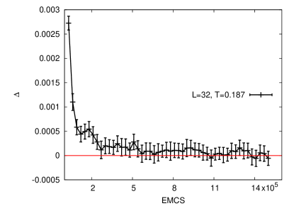
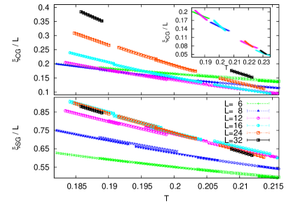
where $U=-\sum_{\langle\boldsymbol{x},\boldsymbol{y}\rangle}J_{\boldsymbol{x},\boldsymbol{y}}\langle\vec{S}_{\boldsymbol{x}}\cdot\vec{S}_{\boldsymbol{y}}\rangle/L^{D}$, the link-overlap is $q_{l}=2\sum_{\langle\boldsymbol{x},\boldsymbol{y}\rangle}\langle\vec{S}^{a}_{\boldsymbol{x}}\cdot\vec{S}^{a}_{\boldsymbol{y}}\rangle\langle\vec{S}^{b}_{\boldsymbol{x}}\cdot\vec{S}^{b}_{\boldsymbol{y}}\rangle/(zL^{D})$, while $q_{s}=2\sum_{\langle\boldsymbol{x},\boldsymbol{y}\rangle}\langle(\vec{S}_{\boldsymbol{x}}\cdot\vec{S}_{\boldsymbol{y}})^{2}\rangle/(zL^{D})$ ($z=6$ is the lattice coordination number). Now, both $U$ and $q_{s}$ equilibrate easily. Yet, since $q_{l}$ involves two replicas, it slowly grows from zero until its equilibrium value. Thus, a thermalization bias shows up as $\varDelta>0$.LEEYOUNG2 ; HSG-LVSAP ; KATZPALYOUNG The time evolution of $\varDelta$, for $L=32$ at the lowest $T$, is in Fig. 1. Second, we carried out the standard logarithmic data binning: we compare averages over the second half of the Monte Carlo history, with the second fourth, the second eight, and so forth, finding stability for three bins. Third, we checked for compatibility among reweighting extrapolations for contiguous temperatures (our simulations at different $T$ are statistically independent, see Fig. 2).

Figure 1: (color online) Sample-averaged $\varDelta$ defined in the l.h.s. of Eq. (5) vs. Monte Carlo time, as computed for $L=32$ at $T=0.187$ and $D=0.05$. The EMCS was defined in the caption to Table 1. Each point is an average over 3000 consecutive measurements.

IV RESULTS

Figure 2: (color online) Correlation length in units of the lattice size vs. $T$, for all our system sizes at $D=0.05$. Results for both the CG (top), and the SG sectors (bottom). Data patches correspond each to an independent simulation (we used data reweighting SPECTRALDENSITY ). Inset: CG intersections for pairs of sizes $(L,2L)$. The range of $T$ and $\xi_{\mathrm{CG}}/L$ differ from main plot.

Our FSS analysis compares the correlation length in units of the lattice size for pairs of lattices $(L,2L)$.BALLESTEROS ; VICTORAMIT ; QUOTIENTS Dimensionless quantities, such as $\xi/L$, are functions of $L^{1/\nu}(T-T_{\mathrm{c}})$, $\nu$ being the thermal critical exponent. Thus, the two curves intersect at $T_{\mathrm{c}}(L,2L)$, see Fig. 2. $T_{\mathrm{c}}(L,2L)$ differs from $T_{\mathrm{c}}$ due to scaling corrections (but tends to it for large $L$ VICTORAMIT ). Our dimensionless quantities $\xi_{\mathrm{SG}}/L$ and $\xi_{\mathrm{CG}}/L$, produce two $L$-dependent critical temperatures $T_{\mathrm{SG}}(L,2L)$ and $T_{\mathrm{CG}}(L,2L)$. We compute the anomalous dimensions $\eta$ from the scaling of the susceptibilities $\chi$ [take $\boldsymbol{k}=\boldsymbol{0}$ in Eq. (3)]. For large $L$, and $\eta<2$, $\chi$ diverges as $\chi\propto|T-T_{\mathrm{c}}|^{-\nu(2-\eta)}$. For finite $L$, we consider the susceptibility ratio for $\chi_{\mathrm{CG}}$ and $\chi_{\mathrm{SG}}$ (the dots stand for scaling corrections):

$$\left.\frac{\chi(2L)}{\chi(L)}\right|_{T_{\mathrm{c}}(L,2L)}=2^{2-\eta}\,+\ldots\,.$$ (6)

$L$	$T_{\mathrm{SG}}(L,2L)$	$T_{\mathrm{CG}}(L,2L)$	$2-\eta_{\mathrm{SG}}$	$2-\eta_{\mathrm{CG}}$
$6$	$0.251(2)$	$0.187(1)$	$2.031(11)$	$0.360(8)$
$8$	$0.235(1)$	$0.202(1)$	$2.131(9)$	$0.223(8)$
$12$	$0.207(5)$	$0.221(1)$	$2.413(46)$	$0.081(5)$
$16$	$0.179(10)$	$0.233(1)$	$2.639(55)$	$0.030(5)$

Table 3: Size-dependent critical temperatures $T_{\mathrm{SG}}(L,2L)$ and $T_{\mathrm{CG}}(L,2L)$, and anomalous dimensions $2-\eta_{\mathrm{SG}}$ and $2-\eta_{\mathrm{CG}}$, Eq. (6), for the simulations with $D=0.05$. Errors were obtained with jackknife.

We discuss first the CG sector. The inset of Fig. 2 shows an unusual feature: $\xi_{\mathrm{CG}}/L$ at the crossing point $T_{\mathrm{CG}}(L,2L)$ approaches zero for large $L$. This is to be expected only if $\eta\geq 2$:VICTORAMIT if the susceptibility does not diverge at $T_{\mathrm{c}}$, the correlation length in Eq. (4) scales as $\xi/L\sim L^{-(\eta-2)/2}$. Nevertheless, we still find crossings when comparing lattices sizes $L$ and $2L$, see Fig. 2 and also Ref. FUNNY-SCALING, . Crossings are due to the fact that, in the large-$L$ limit, the correlation length in Eq. (4) is divergent in the low-temperature phase. For $T<T_{\mathrm{c}}$, $\xi/L$ grows as $L^{\theta/2}$ (i.e. the correlation function at large distances $r$ goes to a constant with corrections of order $1/r^{\theta}$, see e.g. Ref. JANUS-DECAY, ). Yet, the susceptibility ratio in Eq. (6) is constant for large $L$, even if $\eta>2$. So, $\eta_{\mathrm{CG}}$ in Table 3 approaches $2$ as $L$ grows.

Besides, it is note worthy that, in spite of the smallness of $D$, $T_{\mathrm{CG}}(L,2L)$ for $D=0.05$ is about twice its value for the isotropic model, $T_{\mathrm{CG}}(D=0)\approx 0.13$.HSG-LVSAP In fact, extrapolating the data in Table 3 as $T_{\mathrm{CG}}(L,2L)=T_{\mathrm{CG}}+A/L$ yields $T_{\mathrm{CG}}\approx 0.26$.

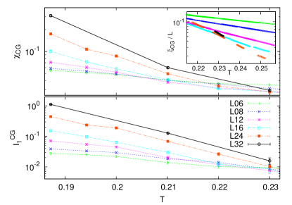
To further investigate the lacking divergence of $\chi_{\mathrm{CG}}$ at $T_{\mathrm{CG}}$, we consider the integrals JANUS-DYNAMICS

$$I_{k}=\sum_{r=0}^{L/2}r^{k}C_{\mathrm{P,P}}(r)\,,$$ (7)

where $C_{\mathrm{P,P}}(r)$ is the plane-to-plane correlation function.FN4 Note that $\chi_{\mathrm{CG}}\sim 2I_{0}$, which means that plane-to-plane correlation functions decays with $r$ slower than the standard point-to-point correlations by a factor $r^{D-1}$. The scaling behavior of the integrals (7) is: $I_{k}\sim constant$ in the paramagnetic phase, $I_{k}\sim L^{k+2-\eta}$ at $T_{\mathrm{CG}}$ (if $k+2-\eta>0$, otherwise it is $I_{k}\sim constant$), and $I_{k}\sim L^{D+k}$ in the CG phase. We show in Fig. 3–top our data for $\chi_{\mathrm{CG}}$ (which is basically $2I_{0}$) and, in Fig. 3–bottom, $I_{1}$. Note that for $T<0.22$ the two integrals are diverging with $L$. On the other hand, for $T=0.22,0.23$, $I_{1}$ grows with $L$, while $\chi_{\mathrm{CG}}$ does not, as expected for $2<\eta_{\mathrm{CG}}<3$.

The behavior of the SG sector is more conventional. A remarkable feature in Fig. 2 and Table 3 is the strong scaling corrections in $T_{\mathrm{SG}}(L,2L)$. We do not consider it safe to extrapolate $T_{\mathrm{SG}}$ to its large-$L$ limit, as we are far from the asymptotic regime. The SG anomalous dimension takes a negative value as $L$ grows (also found in the Ising SG, see e.g. BALLESTEROS ).

An intriguing feature is that $T_{\mathrm{SG}}$ seems smaller than $T_{\mathrm{CG}}$. Indeed, see Fig. 2, at $T\approx 0.187$, where $\xi_{\mathrm{SG}}/L$ becomes $L$-independent, $\xi_{\mathrm{CG}}/L$ is growing fast with $L$. Yet, three caveats prevent us from considering this conclusion as definitive: (i) our lattice sizes are still in a strong cross-over regime, hence the final picture could change as $L$ grows, (ii) the behavior is rather marginal, meaning a larger number of samples would be needed to accurately locate $T_{\mathrm{SG}}$ (this is hardly surprising, given the large value of exponent $\nu$, and the small $\theta$ exponent, for $d=3$ Ising SG’s), and (iii) when considering a larger anisotropy, see below, the effect seems smaller.

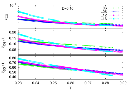
Indeed, we have performed further simulations with $D=0.1$, up to $L=16$. As shown in Fig. 4, the difference between $T_{\mathrm{SG}}$ and $T_{\mathrm{CG}}$ is less clearly defined than for $D=0.05$. On the other hand, the chiral-glass susceptibility is not divergent at the critical point, in agreement with our results for $D=0.05$. Consistently with that, the crossing points for $\xi_{\mathrm{CG}}/L$ shift to a smaller height when $L$ grows.

Figure 3: Chiral glass susceptibility $\chi_{CG}$ (top) and $I_{1}$ integral defined in Eq. 7 (bottom) vs. temperature, for all our system sizes with $D=0.05$. Lines are guides to eyes. Inset: zoom of $\xi_{\mathrm{CG}}/L$ vs. T

Figure 4: For all our lattice sizes at $D=0.1$, we show the chiral-glass susceptibility (top), as well as the CG (center) and SG (bottom) correlation lengths in units of the system size, as a function of temperature.

V CONCLUSIONS

In summary, we have performed a finite size scaling study of the $3d$ Heisenberg spin glass in the presence of a weak random anisotropy, for lattices of size up to $L=32$. Anisotropies cause that the CG susceptibility no longer diverges at $T_{\mathrm{CG}}$, the chiralities ordering temperature. Hence, the anisotropic system belongs to a Universality Class different from the isotropic model (probably that of Ising SG’s). Besides, we found that the spin-glass ordering sets up only at $T_{\mathrm{SG}}<T_{\mathrm{CG}}$. The most economic scenario is that actually $T_{\mathrm{SG}}=T_{\mathrm{CG}}$ (the apparent difference would be due to finite-size effects). In this scenario, chiralities would merely be a composite operator (such as, say, the ninth power of the spin overlap). However, the would-be intermediate temperature region where only chiralities order should be experimentally detectable through the anomalous Hall effect. Numerical studies covering a wider range of values for the anisotropic coupling could also help to elucidate the situation.

References

- (1) See e.g. Spin Glasses and Random Fields, Ed. A. P. Young. World Scientific (Singapore, 1997).
- (2) F. Bert et al., Phys. Rev. Lett. 92, 167203 (2004).
- (3) A. Mauger et al., Phys. Rev. B 41, 4587 (1990).
- (4) W.L. McMillan, Phys. Rev. B 31, 342 (1985); J.A. Olive, A.P. Young and D. Sherrington, ibid 34, 6341 (1986); B.M. Morris et al., J. Phys. C 19, 1157 (1986).
- (5) H. Kawamura, Phys. Rev. Lett. 68, 3785 (1992), ibid 80, 5421 (1998).
- (6) P. M. Levy and A. Fert, Phys. Rev. B23, 4667 (1981).
- (7) A. J. Bray and M. A. Moore, J. Phys. C: Solid State Phys. 15, 3897 (1982).
- (8) F. Matsubara, T. Iyota and S. Inawashiro, Phys. Rev. Lett. 67, 1458 (1991).
- (9) G. Tatara and H. Kawamura, J. Phys. Soc. Jpn. 71, 2613 (2002).
- (10) H. Kawamura, Phys. Rev. Lett. 90, 047202 (2003).
- (11) P. Matl et al, Phys. Rev. B 57, 10248 (1998); J. Ye et al., Phys. Rev. Lett. 83, 3737 (1999); S.H. Chun et al., Phys. Rev. Lett. 84, 757 (2000);
- (12) Y. Taguchi et al., Science 291, 2573 (2001).
- (13) H. G. Ballesteros et al., Phys. Rev. B 62, 14237 (2000).
- (14) H. G. Ballesteros et al., Phys. Lett. B 378, 207 (1996); B387, 125 (1996), Nucl. Phys. B 483, 707 (1997).
- (15) See, e.g., D. Amit and V. Martin-Mayor, Field Theory, the Renormalization Group and Critical Phenomena, (World-Scientific Singapore, third edition, 2005).
- (16) L.W. Lee and A.P. Young, Phys. Rev. Lett. 90, 227203 (2003).
- (17) L.W. Lee and A.P. Young, Phys. Rev. B 76, 024405 (2007).
- (18) I. Campos et al., Phys. Rev. Lett. 97, 217204 (2006).
- (19) D. X. Viet and H. Kawamura, Phys. Rev. Lett. 102, 027202 (2009).
- (20) L. A. Fernandez et al., Phys. Rev. B 80, 024422 (2009).
- (21) F. Matsubara, T. Shirakura and S. Endoh, Phys. Rev. B 64, 092412 (2001); T. Nakamura and S. Endoh, J. Phys. Soc. Jpn. 71, 2113 (2002).
- (22) F. Matsubara, T. Shirakura, S. Endoh and S. Takahashi, J. Phys. A: Math. Gen 36,, 10881 (2003).
- (23) The quasi long-ranged Dzyaloshinskii-Moriya interactions induce an additional crossover, from mean-field to three-dimensional behavior.BRAYMOORE
- (24) I. A. Campbell, and D. Petit, J. Phys. Soc. Jpn. 79, 011006 (2010).
- (25) F. Cooper, B. Freedman and D. Preston, Nucl. Phys. B 210, 210 (1982).
- (26) We will not make any distinction between the CG longitudinal or transversal correlation lengths, see e.g. Ref. LEEYOUNG, , since the two turn out to be compatible within errors.
- (27) F. R. Brown and T. J. Woch, Phys. Rev. Lett. 58, 2394 (1987).
- (28) Eq. (1) can be split as ; is independent of while
- (29) J. H. Pixley and A. P. Young, Phys. Rev. B 78, 014419 (2008).
- (30) J. L. Alonso et al., Phys. Rev. B 53, 2537 (1996); E. Marinari, V. Martin-Mayor and A. Pagnani, ibid 62 (2000) 4999.
- (31) H. G. Ballesteros et al., Nucl. Phys. B 512, 681 (1998).
- (32) M. Falcioni et al., Phys. Lett. B 108, 331 (1982); A. M. Ferrenberg and R. H. Swendsen, Phys. Rev. Lett. 61, 2635 (1988).
- (33) H. G. Katzgraber, M. Palassini and A. P. Young, Phys. Rev. B, 63, 184422 (2001).
- (34) J.L. Alonso et al., Phys. Rev. B 71, 014420 (2005).
- (35) R. Alvarez-Baños et al. (Janus Collaboration), Phys. Rev. Lett. 105, 177202 (2010) and J. Stat. Mech. (2010) P06026.
- (36) F. Belletti et al. (Janus Collaboration), Phys. Rev. Lett. 101, 157201 (2008).
- (37) For planes parallel to (say) the lattice axis, add the correlation function for all pairs of sites , such that , with integer, then divide by . We average over the three lattice directions, as well as over the longitudinal (weight 1/3) and the transversal (weight 2/3) correlation functions.