Fossil Groups Origins: I. RX J105453.3+552102 a very massive and relaxed system at z$\sim$0.5

Abstract

Context. The most accepted scenario for the origin of fossil groups is that they are galaxy associations in which the merging rate was fast and efficient. These systems have assembled half of their mass at early epoch of the Universe, subsequently growing by minor mergers, and therefore could contain a fossil record of the galaxy structure formation.

Aims. We have started an observational project in order to characterize a large sample of fossil groups. In this paper we present the analysis of the fossil system RX J105453.3+552102.

Methods. Optical deep images were used for studying the properties of the brightest group galaxy and for computing the photometric luminosity function of the group. We have also performed a detail dynamical analysis of the system based on redshift data for 116 galaxies. Combining galaxy velocities and positions we selected 78 group members.

Results. RX J105453.3+552102 is located at $\left<z\right>=0.47$, and shows a quite large line–of–sight velocity dispersion $\sigma_{v}\sim 1000$ km s^-1. Assuming the dynamical equilibrium, we estimated a virial mass of $M(<R_{\rm 200})\sim 1$ $\times 10^{15}\;h_{70}^{-1}\;\rm{M_{\odot}}\;$. No evidence of substructure was found within 1.4 Mpc radius. Nevertheless, we found a statistically significant departure from Gaussianity of the group members velocities in the most external regions of the group. This could indicate the presence of galaxies in radial orbits in the external region of the group. We also found that the photometrical luminosity function is bimodal, showing a lack of $M_{r}\sim-19.5$ galaxies. The brightest group galaxy shows low Sèrsic parameter ($n\sim 2$) and a small peculiar velocity. Indeed, our accurate photometry shows that the difference between the brightest and the second brightest galaxies is 1.9 mag in the $r$-band, while the classical definition of fossil group is based on a magnitude gap of 2.

Conclusions. We conclude that RX J105453.3+552102 does not follow the empirical definition of fossil group. Nevertheless, it is a massive, old and undisturbed galaxy system with little infall of $L^{*}$ galaxies since its initial collapse.

1 Introduction

According to current cosmological cold dark matter (CDM) theories, structure in the Universe is built up hierarchically. Thus, virialized CDM halos grow by the merging of smaller virialized halos. Galaxies that populate these halos, also grow hierarchically by the merging of pre-existing galaxies (e.g., White & Rees white78 (1978)). The efficiency of this hierarchical formation depends on several properties of the host dark matter (DM) halo and its satellites, among others: the galaxy number density, galaxy group kinematics, or formation epoch. Nevertheless, it may be possible to find galaxy associations in which the above properties conspire in a way that the merging was fast and efficient. These systems exist in the Universe, and are called fossil groups (FGs).

The first identification of such a system was made by Ponman et al. (ponman94 (1994)), when they suggested that the elliptical galaxy-dominated system RX J1340.6+4018 was probably the relic of what previously constituted a group. Some years later, Jones et al. (jones03 (2003)) gave the first observational definition of FGs. Thus, from the observational point of view, FGs are characterized by the existence of an extreme magnitude gap ($\Delta m_{12}>2$ in the $R$-filter) between the two brightest members of the system within half of its virial radius. These galaxy associations also show an extended bright X-ray emission ($L_{\rm X}>10^{42}$ $h_{50}^{-2}$ erg s^-1) surrounding the brightest group galaxy. According to this definition, these systems are as common as poor and rich galaxy clusters together ($n\sim(1-4)\times 10^{-6}$ $h_{50}^{-3}$ Mpc^-3; Vikhlinin et al. vikhlinin98 (1998); Jones et al. jones03 (2003); Santos et al. santos07 (2007); La Barbera et al. labarbera09 (2009); Voevodkin et al. voevodkin10 (2010)).

Numerical simulations show that FGs could be particular cases of structure formation. Thus, according to these simulations, FGs have been formed inside highly concentrated DM halos at an early epoch of the Universe, assembling half of their dark matter mass at $z>1$, and subsequently growing by minor mergers. In contrast, non-fossil groups show, on average, a later formation (D’Onghia et al. donghia05 (2005); von Benda-Beckmann et al. vonbenda08 (2008)). This early formation leaves enough time for $L^{*}$ galaxies to merge into a massive elliptical-type galaxy located at the center of the group, producing a lack of intermediate-luminosity galaxies and a large magnitude gap between the brightest and the second brightest galaxy of the group. FGs also have special dynamical properties which speed up the merging efficiency. In particular, the in-fall of massive satellites in FGs took place on orbits with low angular momentum, which might be the main responsible of the anisotropy of the group galaxies, in such a way that groups with highly radially anisotropic velocity distributions tend to become fossil (Sommer-Larsen somer06 (2006)). Simulations also indicate that FGs have only been able to accrete on average one galaxy since $z\sim 1$, compared to $\sim 3$ galaxies for normal groups (see von Benda-Beckmann et al. vonbenda08 (2008)). This means that FGs provide unique clues on the history of cosmic mass assembly and the relationship between baryons and their host halos. They also could have a fossil record of the structure formation of galaxies at early epochs of the Universe.

Observations are broadly in agreement with the formation framework of FGs proposed by numerical simulations. Thus, Khosroshahi et al. (khosro07 (2007)) compared the scaling relations of a sample of FGs and non-fossil systems and found that FGs follow the X-ray luminosity-temperature relation ($L_{\rm X}$-$T_{\rm X}$) as clusters and groups. However, there are significant differences in the optical vs. X-ray luminosities ($L_{\rm opt}-$$L_{\rm X}$), X-ray luminosity vs. cluster velocity dispersion ($L_{\rm X}-\sigma$) and X-ray temperature vs. cluster velocity dispersion ($T_{\rm X}-\sigma$) relations. In particular, for a given $\sigma$, FGs are located in more luminous and hotter X-ray halos than normal groups and clusters. They also have larger X-ray luminosities than normal groups for a given $L_{\rm opt}$ (but see also Voevodkin et al. voevodkin10 (2010)). These differences could be due to an early formation epoch of FGs as suggested by simulations (Khosroshahi et al. khosro07 (2007)). Detailed X-ray observations of some FGs also indicate that these systems were assembled at early epochs in high centrally concentrated DM halos with large mass-to-light-ratio ($M/L$) relations. Nevertheless, they do not show cooling cores as those detected in galaxy clusters, which points toward the presence of other heating mechanisms, like AGN feedback (Sun et al. sun04 (2004); Khosroshahi et al. khosro04 (2004),khosro06 (2006); Mendes de Oliveira et al. mendes09 (2009)). The absence of recent galaxy or cluster major mergers together with the lack of cool cores make FGs the ideal objects to study the effects of AGN feedback and the link between galaxy evolution and intra-group medium (IGM).

Optical and near-infrared observations indicate that the faint-end slope ($\alpha$) of the luminosity function (LF) of FGs spans a wide range of values. Thus, the Schechter function fitted to the LF of these systems shows values in the range -1.6$<\alpha<$-0.6 (Cypriano et al. cypriano06 (2006); Khosroshahi et al. khosro06 (2006); Mendes de Oliveira et al. mendes06 (2006), mendes09 (2009)). This suggests that some FGs are dwarf rich systems like similar size/mass galaxy clusters, while others show a lack of dwarf galaxies. It has been pointed out that these differences between fossil and non-fossil systems can reflect different substructure distribution (Jones et al. jones00 (2000)). Thus, FGs could have one order of magnitude less substructure with respect to the standard cosmological model predictions (D’Onghia & Lake donghia04 (2004)). Nevertheless, the number of LFs measured for FGs is scarce and the system where this different substructure was measured has only 40$\%$ of the Virgo mass. It should be pointed out the fact that many systems classified in the past as FGs turned to be fossil clusters. On mass scale of groups it is not completely clear when the transition from galaxy formation to galaxy cluster formation happens. The low mass FGs are intermediate systems in this respect and can give hints of how and at which extent the substructures are accreted. Thus, studies on low mass FGs might give a hint on the abundance of dwarf galaxies in systems with mass scale intermediate between a galaxy and a galaxy cluster as compared to the standard cosmological predictions.

The brightest group galaxies (BGGs) located at the center of FGs are among the most massive galaxies known in the Universe. They contain the key for understanding the formation and evolution of FGs. Observations show that BGGs have also different observational properties than other bright elliptical (E) galaxies. In particular, they present discy isophotes in the center and their luminosity correlates with the velocity dispersion of the group (Khosroshahi et al. khosro06 (2006)). These different properties suggest a different formation scenario for bright Es in fossil and non-fossil systems. While bright Es in FGs would grow by gas-rich mergers, giant Es in non-fossil systems would suffer more dry mergers. However, recent samples of BGGs do not find these differences (La Barbera et al. labarbera09 (2009)).

All previous results have the drawback that they were obtained using small samples of FGs. This could be the reason of some contradictory results found by different studies. The lack of a large and homogeneous statistical study of this kind of systems make the previous results not conclusive. A systematic study of a large sample of FGs remains to be done.

1.1 Fossil Groups Origins (FOGO) project.

We have started a large observing program on FGs. The aim of this project is to carry out a systematic, multiwavelength study of a sample of 34 FGs selected from the Sloan Digital Sky Survey (SDSS; Santos et al. santos07 (2007)). This sample is ideal for providing strong constraints on the observational properties of the galaxy populations in FGs due to its unique characteristics. The sample spans the last 5 Gyr of galaxy evolution ($0<z<0.5$). The groups have a large range of masses and therefore X-ray luminosities (0.04-30 $\times 10^{43}$ erg s^-1). This will be useful for the study of the dependence of FG properties on group mass. Indeed, the absolute magnitude of the central BGGs spans a large range of magnitudes ($-25.3<M_{r}<-21.25$), which will also allow us to analyze the relation of the BGGs and the cluster environment.

The specific scientific goals of this programme are:

• Mass and dynamics of FGs: Given the early assembly of DM halos in FGs, it is reasonable to assume that they are more relaxed systems than non-FGs. Simulations show that using the kinematics of satellite galaxies it is possible to infer their dynamical status and mass distribution all the way to the virial radius. Moreover, the in-fall of $L^{*}$ galaxies occurs along filaments with small impact parameters, increasing the group concentration and therefore its merging efficiency. The signature of this filamentary in-fall could be reflected in the orbital anisotropy of satellite galaxies, which are expected to show an excess of radial anisotropy in their outer regions with respect normal groups (see e.g. Sommer-Larsen 2006). A thorough mass distribution and dynamical study of FGs like that performed by Biviano & Katgert (biv04 (2004)) for galaxy clusters remains to be done.

• Properties of galaxy populations in FGs: These systems are characterized by a large magnitude gap between the two brightest group members. The high luminosity of the BGG combined with the large magnitude gap hint at the merging of the most massive group members. However, little is known about the fate of low-mass satellites in FGs. The faint-end of the LF of low-mass FGs will tell us whether these systems present a paucity of dwarfs (as in the Local Group) or are more similar to dwarf-rich galaxy clusters.

• Formation of the BGG: Understanding the formation of the BGGs is one of the main goals of the project. Simulations indicate that BGGs are the outcome of a process of intense merging between galaxies. Moreover, depending of the gas content of the precursor galaxies, BGGs can present different isophotal structure and AGN activity, given that mergers regulate the formation and fuelling of active nuclei (di Matteo et al. dimatteo05 (2005)). Additionally, the determination of ages, metallicities, $\alpha$-enhancements, and kinematics of their stellar populations will provide strong constraints on the formation history of these unique objects.

• Extended diffuse light: If BGGs are the outcome of intense past merging processes, they are expected to have diffuse and extended stellar haloes. Numerical simulations (Sommer-Larsen somer06 (2006)) show that this diffuse component may contribute up to 40$\%$ of the total $V$-band light of the group, but is only detected at very faint surface brightness ($\sim 26.5$ mag arcsec^-2). This fraction is comparable to or larger than that observed in nearby galaxy clusters and normal groups (Zibetti et al. zibetti05 (2005); Aguerri et al. aguerri05 (2005), aguerri06 (2006); Castro-Rodriguez et al. castror03 (2003), castror09 (2009)). Therefore, the detection of this component is crucial for understanding the formation history of FGs, and to provide an accurate determination of their total baryonic content.

• Connection between BGG and intragroup medium: Numerical simulations and some observational results show that FGs are old and relaxed systems. Therefore, FGs should provide ideal environments for the formation of cool cores as those found in some normal groups and galaxy systems. Nevertheless, so far these cool cores are either not observed in FGs or they are much smaller than expected (Khosroshahi et al. khosro04 (2004), khosro07 (2007); Sun et al. sun04 (2004); Mendes de Oliveira et al. mendes09 (2009)). The absence of major recent galaxy or cluster mergers together with the absence of cool cores make FGs the ideal objects to study the effects of other heating mechanisms, like AGN heating. The AGN feedback would deposit metals and energy into the IGM central gas. The wind metal injection would make the central SN Ia/SN II ejecta of FGs different from that or normal groups and similar size clusters. This scenario will be tested for some of our groups.

• Theory and numerical simulations: the lack of observational data on FGs has so far prevented the validation of most theoretical results. The present programme will provide invaluable information on the mass distribution of FGs, the orbital characteristics of their galaxy populations, the abundance of dwarf galaxies, the amount and distribution of diffuse light, the inner structure of BGGs, and the AGN feedback. This unprecedented data-set is expected to challenge current numerical simulations and serve as reference for future ones.

In order to reach the previous scientific objectives, the Fossil Group Origins (FOGO) project was approved as an International Time Program (ITP) at the Roque de los Muchachos Observatory (ORM) in La Palma, Spain. The multiwavelength observations have been taken during the period 2008–2010. The assigned telescopes for the project were the 4m William Herschel Telescope (WHT), the 3.5m Telescopio Nazionale Galileo (TNG), the 2.5m Isaac Newton Telescope (INT), and the 2.5m Nordic Optical Telescope (NOT). The set of observations include optical and near-IR imaging, multi-object spectroscopy, and integral field spectroscopy.

All FGs from Santos et al. (2007) have been imaged through the sloan $r$-band with the Wide Field Camera (WFC) at INT and the Andalucia Faint Object Spectrograph and Camera (ALFOSC) at NOT. We plan to reach $\mu_{r}\sim 26$ mag arcsec^-2 with $S/N\sim 1$ per pixel. In addition, near-IR images in the $K$-band have been taken for the central regions of 17 groups using The Long-slit Intermediate Resolution Infrared Spectrograph (LIRIS) at the WHT. The multi-object spectroscopy was obtained with the Wide-field Fibre Optic Spectrograph (WYFFOS) at the WHT and the Device Optimized for Low Resolution spectrograph (DOLORES) at the TNG. The target galaxies for the multi-object spectroscopy have been located within 1.4 Mpc radius around the BGG, and with $m_{r}<22$ mag. The selection was done taking into account the photometrical redshift information given by SDSS (see Sec. 2.2). The integral field spectroscopy was obtained with INTEGRAL/WYFFOS mounted at WHT. These observations provide integral field spectroscopy of the central regions of the BGGs.

In this paper we present the first results of the survey with a detailed analysis of the optical images and multi-object spectroscopy of one of the FGs: RX J105453.3+552102. This paper is a pilot program in order to show the capabilities of the FOGO project. The paper is organized as follow. The observations are shown in Section 2. The galaxy catalogues are given in Section 3. The photometric and spectroscopic LFs are shown in Section 4. The photometric properties of the brightest group galaxy are described in Section 5. The internal dynamic of the group is analyzed in Section 6. The discussion and conclusions are given in Section 7.

Unless otherwise stated, we give errors at the 68% confidence level (hereafter c.l.). Throughout this paper, we use $H_{0}=70$ km s^-1 Mpc^-1 in a flat cosmology with $\Omega_{0}=0.3$ and $\Omega_{\Lambda}=0.7$. In the adopted cosmology, 1$\mathrm{{}^{\prime}}\;$corresponds to 353 $h_{70}^{-1}$ kpc  at $z=0.47$, the redshift of the group (see Sec. 3.3).

2 Observations and data reduction

2.1 Optical imaging

Optical imaging of RX J105453.3+552102 was carried out at the 2.5m NOT telescope in March 2008. The data were taken under photometric conditions and a typical seeing of FWHM$\sim$1^′′ during the run. The observations were centered at the position of the BGG ($\alpha(J2000)=10^{\rm{h}}54^{\rm{m}}52^{\rm{s}};\delta(J2000)=+55^{\rm{o}}21^{\prime}12.5^{\prime\prime})$. We used ALFOSC in image mode, with the SDSS $r$-band mounted in the filter wheel. The CCD detector has a size of 2048$\times$2048 pixels, with a plate scale of 0.19 arcsec/pixel, or 5.9 kpc/arcsec at the distance of the group ($z=0.47$). This implies that we have mapped a radius of $\sim 1.1$ Mpc around the BGG.

The data reduction was performed using standard IRAF routines. The bias was subtracted from the images using a master bias obtained by the combination of 10 bias taken at the beginning of the night. We also obtained sky flat images during the twilight. The sky flatfields were combined creating a master flat to correct the images. Some residual light appears in the flat-fielded images. In order to have the best possible flat-field correction of the images, we did a aditional flat-field correction using a super-flat obtained by the combination of the scientific images. The images were observed following a dithering pattern, which turned to be not large enough in order to remove the objects from the images after the combination of all scientific images. In order to remove the objects and create a super-flat we developed our own procedure. The procedure starts by computing the sky background level and its standard deviation ($\sigma_{\rm sky}$) from the biased and flat-fielded images. We adopted the mode of the image as the background level. In the second step we mask out from the scientific images all pixels with 1$\times\sigma_{\rm sky}$ over the sky level. Those pixels were substituted by the value of the sky computed locally. This local background was obtained by measuring the mode in a box of 400-pixels size centered at each of the masked pixels. After several trials, this box size resulted the most appropriate in order to mask the emission from the objects. The masked images were finally combined, resulting a super-flat which contains the large scale light pattern not corrected by the twilight flats. This super-flat was used for a second flat correction of the scientific images. The residual structures in the background of the images were successfully corrected when this super-flat was used.

The bias, flat-field corrected scientific images were astrometrized and register into a common spatial reference. These images were combined into a final $r$-band scientific image with a total exposure time of 2.5 hours and a seeing of 1^′′. Figure 1 shows the $r$-band image of the group and a zoom around the BGG.

The image was calibrated comparing the SDSS $r$-band magnitudes of the stars located in the field of view (FOV) of our image with our instrumental magnitudes. A simple zero-point offset with the SDSS magnitudes was computed in order to calibrate the image. The rms of the calibration turned to be 0.08 mag.

2.2 Spectroscopic data

Multi–object spectroscopic observations of RX J105453.3+552102 were carried out at the TNG telescope in February 2008. We used DOLORES in the Multi Object Spectroscopic mode (MOS) with the LR–B Grism 1, yielding a dispersion of 187 Å/mm. We used the new E2V CCD detector with a pixel size of 13.5 $\mu$m. The CCD is a matrix of $2048\times 2048$ pixels. We observed five MOS masks for a total of 151 slits. We acquired 4 exposures of 1800 s for three masks and 5 exposures of 1800 s for two masks. Wavelength calibration was performed using Helium–Argon lamps. Reduction of spectroscopic data was carried out with the IRAF package.

The target selection for the multi–object spectroscopy was based on the SDSS database. We downloaded a catalogue with all galaxies with $m_{r}<22$ mag which are located within a radius of 1.4 Mpc around the BGG at the distance of the group. In a second step, we selected the galaxy targets using the photometric redshift information provided by SDSS. We selected as possible targets galaxies with 0.37$<z_{\rm phot}<0.57$. This range of photometrical redshift was chosen because the group, according to the spectroscopic redshift of the BGG provided by SDSS, is located at $z=0.47$ and the typical photometric redshift error from SDSS is about 0.1. Figure 2 shows the color-magnitude diagram of the galaxies located within 1.4 Mpc radius from the group center. The magnitudes in the $g$ and $i$ bands were obtained from the SDSS database. The figure also shows the targets selected for the multi–object spectroscopy.

Radial velocities, $\rm v=cz$, of the selected galaxies were determined using the cross–correlation technique (Tonry & Davis ton79 (1979)) implemented in the IRAF package RVSAO (developed at the Smithsonian Astrophysical Observatory Telescope Data Center). Each spectrum was correlated against six templates for a variety of galaxy spectral types: E, S0, Sa, Sb, Sc, Ir (Kennicutt ken92 (1992)). The template producing the highest value of $\cal R$, i.e., the parameter given by RVSAO and related to the signal–to–noise ratio of the correlation peak, was chosen. Moreover, all the spectra and their best correlation functions were examined visually to verify the redshift determination. In 24 cases (see Table Fossil Groups Origins: I. RX J105453.3+552102 a very massive and relaxed system at z$\sim$0.5) the redshift of the galaxies was determined by the emission lines observed in the wavelength range of the spectra (EMSAO procedure).

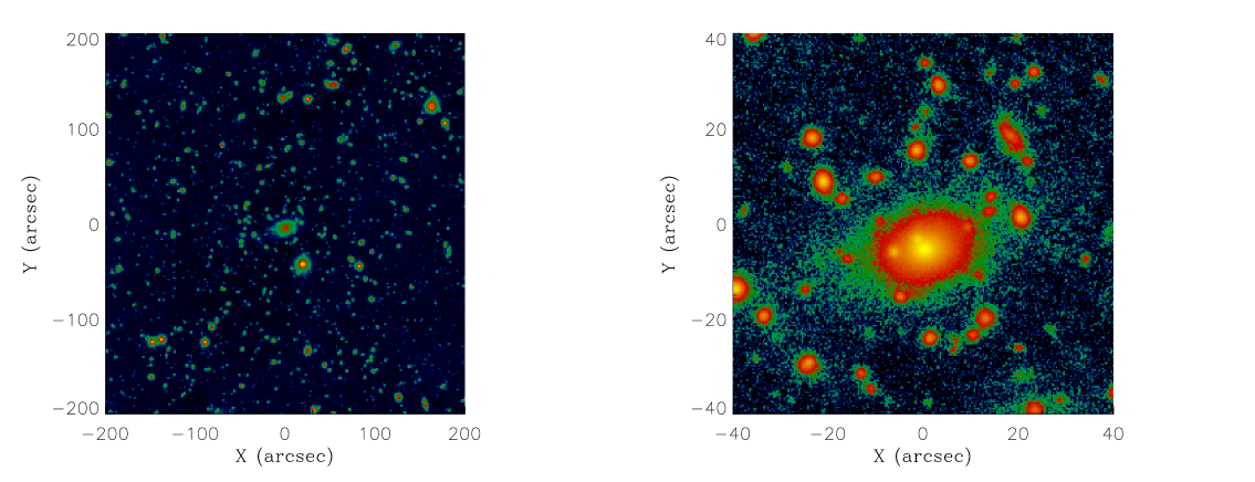
Figure 1: (left panel) $r$-band images of RX J105453.3+552102; (right panel) zoom of the central region of the group. In both panels North is up and east is left.

3 Galaxy catalogues

Two different catalogues were obtained. One catalogue contains the photometry of the galaxies located in our $r$-band image. This catalogue was used to compute the photometric luminosity function of the group. The other catalogue contains the velocity information of the galaxies observed in the MOS observations. This will be used for determining the group members, the spectroscopic luminosity function and the dynamics of the group.

3.1 Photometric galaxy catalogue

The photometric galaxy catalogue was obtained using SExtractor (Bertin & Arnouts ber96 (1996)). SExtractor identifies objects and measures their flux in astronomical images. Here we discuss those parameters of SExtractor that are relevant for the identification and flux measurements of our objects.

Objects were identified as imposing that they cover a certain minimum area and have number counts above a limiting threshold taking the sky local background as a reference. The limiting size and fluxes were 25 pixels and one standard deviation of the sky counts, respectively. The selected limiting size corresponds to an apparent size of 1 arcsec, which is about the size of the seeing disc. We have performed careful visual inspections of the frames in order to deal with the best combination of the above parameters that remove spurious objects from the catalogues. The resulting photometric catalogue contains 957 objects. For each object we measured three different magnitudes. Two of them were aperture magnitudes with diameters: 5.6 and 15 pixels. The smallest diameter corresponds to a circular aperture of area equal to the minimum detection area in SExtractor, and the largest one to an aperture of radius 3$\sigma$, being $\sigma$ the standard deviation of the Gaussian seeing point spread function (PSF) of the image. We have also included in the catalogue the $MAG-AUTO$ magnitude given by SExtractor. This magnitude is computed in a elliptical aperture enclosing the flux of each object.

The separation between galaxies and stars was performed on the basis of the SExtractor stellarity index ($S/G$). Objects with $S/G$ close to 1 correspond to stars while galaxies are those with $S/G$ close to 0. This separation is clear for bright objects. In contrast, a correct classification is more difficult for faint objects. In order to be conservative, we have determined stars as those objects with $S/G>$0.85.

We have determined the completeness of our photometric data following the same criteria as Sánchez-Janssen et al. (sanchez05 (2005)). Thus, for all the detected objects we computed the mean central surface brightness ($\mu_{o}$) measured in a circular aperture of area equal to the minimum detection area used in SExtractor. Figure 3 shows $\mu_{o}$ as a function of the apparent $r$-band magnitude ($m_{r}$) of the detected objects. We have overplotted with crosses those objects with $S/G>0.85$ corresponding to stars. Notice that stars (objects with $S/G>0.85$) are located in the upper diagonal of the plot. In contrast, the galaxies (objects with $S/G<0.85$) are located in the broader region of the plot. We have computed the central surface brightness which correspond to 1$\sigma_{\rm sky}$ detection limit used by SExtractor resulting $\mu_{o}=27.4$ mag arcsec^-2 (horizontal line in Fig. 3). Given the distribution of the objects in Fig. 3 we can conclude that our photometric limiting magnitude is $m_{r}\sim 24.0$ mag.

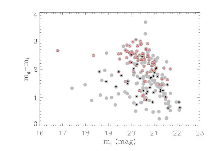
Figure 2: (Color-magnitude diagram of the SDSS galaxies located within 1.4 Mpc around the BGG (grey large circles). The black points (non cluster members) and red triangles (cluster members) represent the galaxies selected for the spectroscopy.

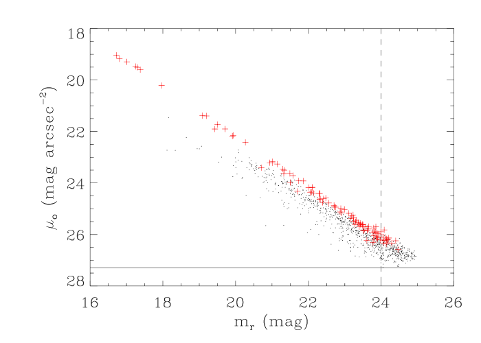
Figure 3: The aperture central surface brightness versus apparent magnitude of the detected objects. Crosses represent stars (objects with $S/G>0.85$) and points correspond to galaxies (objects with $S/G<0.85$). The horizontal line correspond to 1$\sigma_{\rm sky}$ isophotal detection limit used in SExtractor. The vertical dashed line is our limiting magnitude.

3.2 Spectroscopic galaxy catalogue

The spectroscopic catalogue was formed by the galaxies with measured radial velocities from our MOS observations. Our spectroscopic survey in the field of RX J105453.3+552102 consists of spectra for 116 single galaxies, of which 18 (4) have double (triple) measurements as coming from five different masks. The nominal errors as given by the cross–correlation are known to be smaller than the true errors (e.g., Malumuth et al. mal92 (1992); Bardelli et al. bar94 (1994); Ellingson & Yee ell94 (1994); Quintana et al. qui00 (2000)). Double/triple redshift determinations for the same galaxy allow to estimate more reliable errors. Previous analyses on data acquired with the same instrumentation and of comparable quality showed that nominal errors obtained through the RVSAO procedure should be multiplied by a factor $\sim 2$ (Barrena et al. bar09 (2009) and references therein). Following the method of Barrena et al. (bar09 (2009)), we compared the determinations coming from different masks and found that the nominal errors were underestimated by a factor 2 in our case, too. Therefore, we assumed that the true errors are larger than nominal cross–correlation error by a factor of 2. To check the errors obtained trough the EMSAO procedure we had only three galaxies with double determinations. To be conservative we assumed that errors on $cz$ recovered from EMSAO are $\sim$ 100 km s^-1.

As for the compilation of our spectroscopic catalogue, for all the galaxies with multiple redshift estimates we used the weighted mean of the multiple measurements and the corresponding errors. The median error on $cz$ was 98 km s^-1. The redshift distribution of the 116 galaxies having robust radial velocity measurements is shown in Fig. 4.

We measured redshifts for galaxies down to magnitude m${}_{r}\lesssim$ 22 mag. Nevertheless, the median completeness of the observations was 84$\%$, being $100\%$ only for galaxies with magnitude m${}_{r}\lesssim 18.5$ mag (see Fig. 5). This spectrocopic completeness will be taken into account for the computation of the spectroscopic LF of the group (see Sect. 4).

Figure 4: Redshift galaxy distribution. The thick solid line histogram refers to the 83 galaxies assigned to the RX J105453.3+552102 complex according to the DEDICA reconstruction method.

Figure 5: Completeness of MOS observations (see text for more details).

Table Fossil Groups Origins: I. RX J105453.3+552102 a very massive and relaxed system at z$\sim$0.5 lists the photometric and kinematic properties of the galaxies with MOS data. The columns indicate: (Col 1) galaxy name; (Col 2) our SExtractor $r$ band magnitude (the error of this magnitude is in the range 0.08-0.1 mag for all objects); (Col 3) line-of-sight velocity $v=cz$; (Col 4) 1=cluster member, 0=non cluster member; (Col 5) comments: E=redshift measured using emission lines; NE= galaxies with no envidence of obvious emission lines; (Col 6-10) $ugriz$ SDSS model magnitudes.

3.3 Member selection

To select group members out of 116 galaxies having redshifts, we followed a two steps procedure. First, we performed the 1D adaptive–kernel method (hereafter DEDICA, Pisani pis93 (1993) and pis96 (1996); see also Fadda et al. fad96 (1996); Girardi et al. gir96 (1996)). We searched for significant peaks in the velocity distribution at $>$99% c.l.. This procedure detects RX J105453.3+552102 as a peak at $z=0.47$ populated by 83 galaxies considered as candidate group members (in the range $0.456<z<0.502$, see Fig. 4). Out of 33 non members, 26 and 7 were foreground and background galaxies, respectively. Notice the advantage of including the photometrical redshifts in the selection of the spectroscopical targets. Thus, 88$\%$ of the galaxies have redshifts in the range 0.37$<z<$0.57, the range of photometric redshifts we selected. Indeed, 70$\%$ of all measured redshifts correspond to actual members.

All the galaxies assigned to the group peak were further analyzed in the second step which uses the combination of position and velocity information: the “shifting gapper” method by Fadda et al. (fad96 (1996)). This procedure rejects galaxies that are too far in velocity from the main body of galaxies within a fixed bin that shifts along the distance from the group center. The procedure is iterated until the number of group members converges to a stable value. For the center of RX J105453.3+552102 we adopted the position of the BGG. Fadda et al. (fad96 (1996)) used a gap of $1000$ km s${}^{-1}\;$in the cluster rest–frame and a bin of either 0.6 $h_{70}^{-1}$ Mpc, or large enough to include 15 galaxies, these parameters well working in their cluster sample. For RX J105453.3+552102 this choice of the parameters rejects six galaxies (see Fig. 6). Out of these, the closest to the group center (ID SDSS J105454.00+552129.2) is very close to the main body of galaxies and would be not rejected in the case of a small - comparable to typical $cz$-error - change of the gap parameter (i.e. a gap of $1080$ km s${}^{-1}\;$instead of $1000$ km s^-1). Moreover, the central velocity dispersion in a galaxy system is often found to be larger than in outer regions (den Hartog & Katgert den96 (1996); Rines et al. rin03 (2003); Aguerri et al. aguerri07 (2007)). For the above reasons, we preferred to be more conservative and did not reject the galaxy ID SDSS J105454.00+552129.2. This leads to a sample of 78 fiducial members. We verified that the exclusion/inclusion of the above galaxy does not change the results of our dynamical analysis.

Figure 6: The 83 galaxies assigned to the RX J105453.3+552102 density peak in Fig. 4. Crosses indicate galaxies which were considered as interlopers on the basis of the gapper method. Circles indicate the 78 fiducial group members. The galaxy with the double symbol (i.e. SDSS J105454.00+552129.2) was not rejected to be more conservative. This choice did not affect the results of our dynamical analysis.

4 Photometric and spectroscopic luminosity functions of the group

We have computed the photometric and spectroscopic luminosity functions of RX J105453.3+552102. The photometric luminosity function (LF_phot) was obtained as the statistical difference between the galaxy counts in the group and control field samples. The selection of the control field is critical since it will influence in the measurements of the parameters of the LF_phot. In order to have a robust determination of the parameters of the LF_phot, several control field samples were used. One of these control fields was observed by us the same night of the observations under the same instrumental and atmospheric conditions as the scientific images. However, this control sample is not so deep as the scientific image. Indeed, it limiting magnitude $m_{r}\sim 23$ mag, about 1 mag brighter than the limiting magnitude of the scientific image. Therefore we have also used deeper backgrounds than our control field from the literature: Capak et al. (capak04 (2004)), Yasuda et al. (yasuda01 (2001)), Huang et al. (huang01 (2001)), and Metcalfe et al. (metcalfe01 (2001)). All these control fields allowed us to obtain a statistical subtraction of the background galaxy counts down to our limiting magnitude. Figure 7 shows all the different backgrounds used in this work as well as the mean background which was used for the computation of the LF_phot.

Figure 8 shows the photometric luminosity function of RX J105453.3+552102 obtained as the statistical difference between the galaxy counts of the group and the background galaxy counts (full black points). Notice that the photometric information for the group galaxies goes down to $\sim 5$ magnitudes fainter than the bright cut-off of the LF. This is one of the deepest photometric LFs of galaxies in a cluster at z$\sim 0.5$ (see also Rudnick et al. rudnick09 (2009)).

The galaxy LF_phot shown in Fig. 8 was determined by using all galaxies within 1 and 0.5 Mpc radius from the BGG, respectively. Notice that in the brightest magnitude bin of the LF computed with galaxies within 1 Mpc radius there is more than one galaxy after the statistical subtraction of the background galaxies. Two of these bright galaxies are located at a distance larger than 500 kpc from the center of the group. This do not invalid the selection of this group as FG. Indeed, according to the SDSS photometric redshifts these two bright galaxies are foreground objects. The galaxy LF_phot was fitted with a Schechter function (Schechter schechter76 (1976)):

$$\phi(m_{r})=\phi^{*}\times[10^{0.4(m^{*}-m_{r})}]^{\alpha+1}e^{-10^{0.4(m^{*}-m_{r})}},$$ (1)

where $\alpha$ is the slope of the faint end of the LF, $m^{*}$ is the characteristic magnitude and $\phi^{*}$ is a normalization factor. The fit of the Schechter function to the data was done by minimizing the $\chi^{2}$ by taking errors into account and assigning a statistical weight to each of the points. The best-fit parameters are written in Fig. 8.

In order to check the strength of our LF_phot we have computed another LF using a different technique. In this case, members were selected using the photometric redshifts provided by SDSS. We have downloaded a catalogue with all the galaxies detected by SDSS-DR7 within a radius of 1 Mpc around the BGG of RX J105453.3+552102. We considered as foreground and background galaxies those with $z_{\rm phot}<0.37$ or $z_{\rm phot}>0.57$, respectively. The limits in the $z_{\rm phot}$ were chosen taking into account that the typical errors of SDSS $z_{\rm phot}$ are $\sim 0.1$. This field galaxy sample was used for computing a new photometric LF (red squares in Fig. 8; hereafter LF_SDSS). Notice the agreement between LF_SDSS and LF_phot.

The spectroscopic luminosity function (LF_spec) was determined using the velocities measured from our MOS observations. This LF was computed taking into account the group members and the selection function (i.e., the number of galaxies with redshift information over the number of possible spectroscopic targets per magnitude bin). Figure  8 shows LF_spec (green diamonds). Notice the good agreement within the errors between LF_phot, LF_SDSS, and LF_spec down to $M_{\rm r}\sim-21$, the limiting magnitude of our LF_spec.

We have integrated the fitted Schechter function in the $r$-band in order to obtain the total luminosity of the group. We have added the luminosity of the BGG, since this galaxy was not considered in the fit of the LF_phot.Thus, the total luminosity of the group, within 1 Mpc radius, turned to be $L_{r}=2.0\times 10^{12}$ L_⊙. The BGG accounts for $14\%$ of the total group luminosity. This percentage increases up to $32\%$ when only galaxies within 0.5 Mpc from the group center were considered.

Figure 8 also shows a prominent dip in the LF_phot at $M_{r}\sim-19.5$. The dip is more clear in the LF_phot computed with the galaxies within 0.5 Mpc radius. This indicates that there is a lack of galaxies with $M_{r}\sim-19.5$ in the innermost regions of the group.

The photometric LFs are very sensitive to the background subtraction. In particular, the mean background used in the present work could affect to the dip detected in the LF_phot. In order to check the dependence of this dip with the galaxy background used we have obtained the photometric LF of the group using only our own background. This background was taken in similar conditions as the observations and is deep enough in order to see the presence of the dip. This new LF_phot also showed the dip at $M_{r}\sim-19.5$. This indicates that the dip does not depend on the adopted galaxy background.

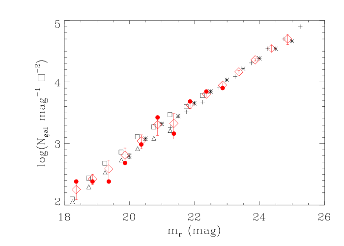
Figure 7: Background galaxy number counts from: our control field (full points), Capak et al. (2004) (asterisks), Yasuda et al. (2001) (triangles), Huang et al. (2001) (squares), and Metcalfe et al. (2001) (crosses). The diamonds represent the mean background used for the photometric luminosity function.

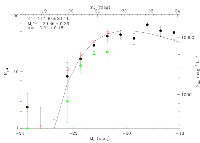
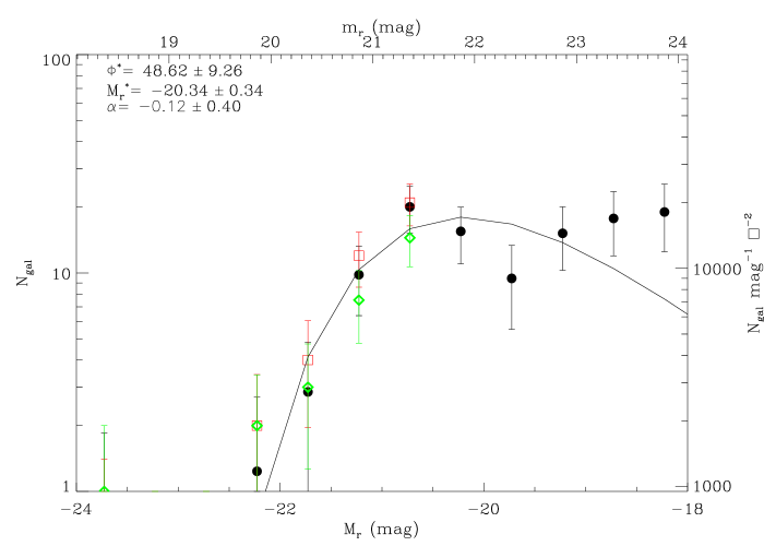
Figure 8: Luminosity function of the galaxies of RX J105453.3+552102 within 1 Mpc (top panel) or 0.5 Mpc (bottom panel) radius, respectively. In all panels, the black points represent $\rm LF_{\rm phot}$ calculated by the statistical subtraction of galaxy counts obtained from the literature. The red squares represent $\rm LF_{\rm phot}$ in which the background counts were obtained using the photometric redshift from SDSS. The green diamonds represent $\rm LF_{\rm spec}$.

5 Photometric properties of the brightest group galaxy

We have fitted ellipses to the isophotes of the brightest group galaxy of RX J105453.3+552102. The fits were done using the ELLIPSE task from the IRAF package which uses the iterative algorithm described by Jedrzejewski (jedr87 (1987)). Figure  9 shows the $r$-band surface brightness (dimming corrected), ellipticity, and position angle radial profiles of the fitted ellipses. Our surface photometry extends out to $\sim 130$ kpc from the galaxy center. At this distance, the $r$-band surface brightness of the BGG is $\mu_{r}\sim 27.0$ mag arcsec^-2. The ellipse fitting algorithm converged for galactrocentric radius smaller than $\sim 80$ kpc. The surface brightness of the isophotes with larger radius was obtained by imposing that the ellipticity and position angle were equal to those of the isophote with 80 kpc. These values were 0.42 and 106.8^∘ for the ellipticity and position angle, respectively. Figure  9 also shows that the isophotal ellipticity profile of the BGG increases with radius and there is a twist of $\sim 10^{\circ}$ between the inner isophotes ($R>$10 kpc) and the outer ones ($R>40$ kpc). The difference between the inner and outer regions of the galaxy can be also seen in the change of the coordinates of the isophote center at radii larger than $\sim 60$ kpc (see Fig.  9). This change in the isophotal center could be due to some tidal distortion in the outermost regions of the BGG.

Figure  9 also shows the radial profile of the Fourier coefficient $a_{4}$ of the isophotes of the BGG. This coefficient is related with the isophotes shape. Negative values of $a_{4}$/$a$ indicates boxy isophotes. In contrast, $a_{4}/a>0$ is related with discy ones. We can see that the $a_{4}/a$ radial profile of the BGG of RX J105453.3+552102 is close to zero in the inner $\approx 80$ kpc, and takes positive values in the outermost regions of the galaxy (R$>$80 kpc). This parameter also indicates different photometric properties of the internal and external regions of the galaxy

We have fitted a two-dimensional Sèrsic model to the surface brightness of the BGG. The fit was done using the automatic fitting routine GASP2D (Méndez-Abreu et al. mendez08 (2008)). Figure  9 shows the fitted model and the residuals of the fit. We have also overploted in Fig.  9 the one-dimensional fitted Sèrsic surface brightness profile to the isophotal surface brightness profile. Notice that the agreement between observations and model is remarkable. The surface brightness profile of the BGG is well fitted with a single Sèrsic profile. This fit reports a total magnitude of $m_{r}=17.49$ for the BGG. There is no extra light over the Sèrsic profile in the outermost regions of the galaxy. This indicates that this galaxy is not a cD galaxy (see Graham et al. graham96 (1996); Nelson et al. nelson02 (2002); Gonzalez et al. gonzalez05 (2005); Patel et al. patel06 (2006); Seigar et al. seigar07 (2007); Vikram et al. vikram10 (2010)). It is also interesting to note that the fitted Sèrsic profile has $n\sim 2$. According to the magnitude-$n$ relation follow by spheroidal galaxies we should expect a larger value of $n$ (see e.g., Aguerri et al. aguerri04 (2004), and references therein). Recently, it has been found that the Sèrsic shape parameter of massive early-type galaxies is smaller for galaxies at higher redshift (van Dokkum et al. vandokkum10 (2010); Vikram et al. vikram10 (2010)). Nevertheless, at $z\sim 0.5$ there are no galaxies in the sample by van Dokkum et al. (2010) with $n\sim 2$. Only galaxies at $z\sim 2$ and extremely compact show values of $n\sim 2$ (see fig. 7 van Dokkum et al. vandokkum10 (2010)). These structural differences of the BGG with respect to other bright early-type galaxies could indicates a different formation. In particular, the low value of $n$ unveil the kind of mergers that have formed the galaxy. In order to get a similar light profile it is required a very gas rich merger for the progenitors ($\sim 80\%$ gas rich; see Hopkins et al. hopkins08 (2008)).

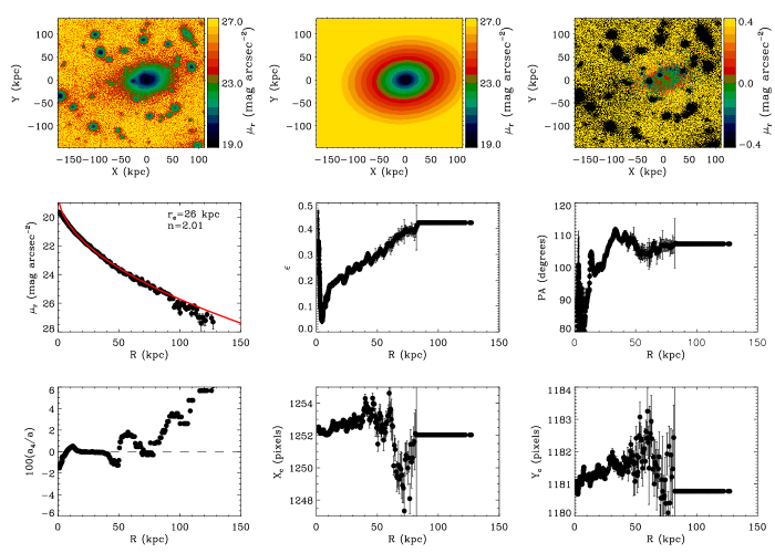
Figure 9: Photometric properties of the BGG of RX J105453.3+552102. Top panels: $r$-band image of the BGG (left), 2D Sèrsic fitted model (center), and residuals of the fit (right). Middle panels: isophotal $r$-band dimming corrected surface brightness and unconvolved Sèrsic fitted model (left), ellipticity (center) and position angle (right) radial profiles of the BGG. Bottom panels: isophotal $a_{4}$ parameter (left), X coordinate (center), and Y coordinate (right) of the center of isophotes as a function of the galactrocentric distance.

6 Internal dynamics

6.1 Global dynamical properties

Figure 10 shows the velocity distribution of the 78 member galaxies. By applying the bi-weight estimator to the 78 member galaxies (ROSTAT package; Beers et al. bee90 (1990)), we computed a mean redshift of $\left<z\right>=0.4661\pm$ 0.0004, i.e. $\left<\rm{v}\right>=(139731\pm$110) km s^-1. We estimateed the line–of–sight (LOS) velocity dispersion, $\sigma_{v}$, by using the bi-weight estimator and applying the cosmological correction and the standard correction for velocity errors (Danese et al. dan80 (1980)). We have obtained $\sigma_{v}=969_{-85}^{+107}$ km s^-1, where errors were estimated through a bootstrap technique. This velocity dispersion does not significantly change when we exclude the six blue galaxies (m_g-m${}_{i}<1.5$). In this case, $\sigma_{v}=993_{-87}^{+119}$ km s^-1.

To evaluate the robustness of the $\sigma_{v}$ estimate we analyzed the velocity dispersion profile (Fig. 11). The integral pigrofile is almost flat. This indicates that a robust value of $\sigma_{v}$ is already reached in the internal regions (e.g., Fadda et al. fad96 (1996); Girardi et al. gir96 (1996)).

In the framework of usual assumptions: i) system sphericity; ii) dynamical equilibrium; iii) the galaxy distribution traces the mass distribution, one can compute virial global quantities. Following the prescriptions of Girardi & Mezzetti (gir01 (2001)), we assumed for the radius of the quasi–virialized region $R_{\rm vir}=0.17\times(\sigma_{v}/{\rm km\leavevmode\nobreak\ s^{-1}})/H(z)\times{\rm Mpc}=1.83$ $h_{70}^{-1}$ Mpc (see their Eq. 1 with the scaling with $H(z)$; see also the Eq.  8 of Carlberg et al. car97 (1997) for $R_{200}$). We have redshifts for galaxies out to a radius of $R_{\rm out}\sim 1.37$ $h_{70}^{-1}$ Mpc sampling the region within $\sim 0.76\times R_{\rm vir}$.

One can compute the virial mass (Limber & Mathews lim60 (1960); see also, e.g., Girardi et al. gir98 (1998)) using the data for the $N_{\rm g}$ observed galaxies:

$$M=3\pi/2\cdot\sigma_{v}^{2}R_{\rm PV}/G-\rm{SPT},$$ (2)

where SPT is the surface pressure term correction (The & White the86 (1986)), and $R_{\rm PV}$, equal to two times the (projected) mean harmonic radius, is:

$$R_{\rm PV}=\frac{N_{\rm g}(N_{\rm g-1})}{\Sigma_{\rm j<\rm i}\Sigma_{\rm i}R_{\rm ij}^{-1}},$$ (3)

where $R_{\rm ij}$ is the projected distance between two galaxies.

The estimate of $\sigma_{v}$ is a robust estimate in RX J105453.3+552102 (see Fig. 11) and thus we considered our global value. The value of $R_{\rm PV}$ depends on the size of the sampled region and possibly on the quality of the spatial sampling, e.g. whether the galaxy sample suffer of radial-dependent incompleteness. In particular, ignoring the problem of radial-dependent incompleteness can have quite a catastrophic effect on the cluster mass estimate (see Sect. 4.4 of Biviano et al. biv06 (2006)). We verified that our sample is not biased comparing the distribution of cluster-centric distances of galaxies having redshift vs. those of all SDSS galaxies having $0.37<z_{\rm phot}<0.57$ (no difference according to the Kolmogorov-Smirnov test, hereafter 1DKS–test; see e.g., Press et al. pre92 (1992)). For our sampled region, i.e. within $R_{\rm out}$ we obtain $R_{\rm PV}=(1.21$$\pm$0.09) $h_{70}^{-1}$ Mpc, where the error was obtained via a jackknife procedure (see e.g., Press et al. 1992). The value of SPT correction strongly depends on the amount of the radial component of the velocity dispersion at the radius of the considered region and could be obtained by analyzing the velocity–dispersion profile, although this procedure would require several hundreds of galaxies. Combining data of many clusters it results that velocities are isotropic and that the SPT correction at $\sim R_{\rm 200}$ is $\rm{SPT}/M_{\rm v}\sim 20\%$ (e.g., Carlberg et al. car97 (1997); Girardi et al. gir98 (1998)). Applying the same correction to our mass estimate we obtained $M(<R_{\rm out})=(1.0\pm 0.2)$ $\times 10^{15}\;h_{70}^{-1}\;\rm{M_{\odot}}$.

Figure 10: Upper panel: Rest–frame velocity histogram for the 78 group members. The arrow indicates the velocity of the BGG. Lower panel: Stripe density plot where the arrows indicate the positions of the significant gaps.

Figure 11: Differential (big circles) and integral (small points) profiles of mean velocity (upper panel) and LOS velocity dispersion (lower panel). The differential radial profiles were obtained by averaging velocities and velocity dispersions in four 0.35 $h_{70}^{-1}$ Mpc wide annuli. The integral radial profiles were obtained by averaging velocities and velocity dispersions within each (projected) radius. The first values are computed on the five galaxies closest to the center. The errors are the $68\%$ c.l.

To obtain the mass within the whole virialized region, which is larger than that sampled by observations we used an alternative estimate of $R_{\rm PV}$ on the basis of the knowledge of the galaxy-number distribution. Following Girardi et al. (gir98 (1998); see also their approximation given by Eq. 13 when $A=R_{\rm vir}$) we assumed a King–like profile with parameters typical of galaxy clusters: a core radius $R_{\rm c}=1/20\times R_{\rm vir}$ and a slope–parameter $\beta_{\rm fit}=0.8$, i.e. the volume galaxy-number density at large radii goes as $r^{-3\beta_{\rm fit}}=r^{-2.4}$. Notice that the same values of $R_{\rm c}$ and $\beta_{\rm fit}$ were also found by directly fitting the data of RX J105453.3+552102. We obtained $R_{\rm PV}(<R_{\rm vir})=1.36$ $h_{70}^{-1}$ Mpc, where a $25\%$ error was expected (Girardi et al. gir98 (1998)). Assuming the $20\%$ SPT correction we computed $M(<R_{\rm vir})=1.1_{-0.3}^{+0.4}$ $\times 10^{15}\;h_{70}^{-1}\;\rm{M_{\odot}}$.

Adopting a completely different approach based on numerical N-body simulations, we used the Eq. 2 of Biviano et al. (biv06 (2006)), opportunely rescaled for cluster redshift and our cosmology

$$M_{\rm v}(<R_{\rm v})=11.13(\sigma_{v}/10^{3}{\rm km\ s^{-1}})^{3}\times H_{0}/H(z)\times 10^{14}\;h_{70}^{-1}\;\rm{M_{\odot}},$$ (4)

to compute a mass estimate $M_{\rm v}(<R_{\rm v}=1.62\;h_{70}^{-1}\mathrm{Mpc})=7.9$ $\times 10^{14}\;h_{70}^{-1}\;\rm{M_{\odot}}$, where $R_{\rm v}$ is another estimate for $R_{200}$. Notice that, although this and the above empirical procedure differ in fixing the value of $R_{\rm 200}$, the two mass estimates only differ for $\sim 10\%$ when rescaled to the same radius.

6.2 Velocity distribution

We have analyzed the velocity distribution to look for possible deviations from Gaussianity that can be interpreted as the signature of a complex dynamics. For the following tests the null hypothesis is that the velocity distribution is a single Gaussian.

We estimated three shape estimators, i.e. the kurtosis (KURT), the skewness (SKEW), and the scaled tail index (STI) using the ROSTAT package and we computed the significance levels according to Beers et al. (bee91 (1991); see their Table 2). The scale tail index (STI=1.152) and the normalized kurtosis (KURT=0.370) turned to be consistent with a Gaussian. In contrast, the skewness (SKEW=0.454) shows evidence of departure from a Gaussian (with a c.l. in the $95-99\%$ range). However, as noticed by Beers et al. (bee91 (1991)), the STI index is a conservative diagnostic for studying galaxy clusters, while the coefficients of skewness and kurtosis are biased toward falsely significant values. In our case, the rejection of only one galaxy (i.e., SDSS J105454.00+552129.2) which is at the border line of our member selection (see § 3.3), leads to SKEW=0.242 which is fully consistent with a Gaussian velocity distribution.

It is possible to interpret the shape of the velocity distribution as a rough indicator of the orbital anisotropy of the group members. Thus, the halo of a dynamically hot system with isotropic orbits and a constant circular velocity curve (i.e., with a massive dark matter halo) has a Gaussian LOS velocity distribution and KURT=0 (see Gerhard 1993). Instead, a system containing objects on radial orbits tend to produce a centrally peaked LOS velocity distribution with long tails, resulting in a positive value of kurtosis. As discussed earlier, the degree of fossilness might reside in the presence of radial orbits in the outer group regions. For this reason we have attempted to look for signatures of non-Gaussianity in the group outskirts by dividing the spectroscopic sample in three radial bins (with 26 members each), and recomputed the kurtosis parameter for each bin. Due to the small number statistics, we have used a bootstrap approach to carefully take into account the effect of the binning and the presence of outliers. The final result is that the first two radial bins ($R\sim 0.5^{\prime},1.5^{\prime}$) the kurtosis turned out to be still fully consistent with a Gaussian distribution, while in the third bin, which includes objects with $R>2^{\prime}$, we have found KURT$=1.0^{+0.9}_{-0.7}$ with errors accounting 10$\%$ and 90$\%$ quartiles over 500 bootstrap experiments. This results suggest that there is a statistically significant departure from Gaussianity of the group member velocities outside $R=2^{\prime}$, which we interpret as a hint of radial orbits at these radii. However a full assessment on the actual amount of anisotropy of the system will require a more detailed dynamical analysis, which is beyond the purpose of this paper.

We also investigated the presence of gaps in the velocity distribution. We followed the weighted gap analysis presented by Beers et al. (bee91 (1991); bee92 (1992); ROSTAT package). We looked for normalized gaps larger than 2.25 since in random draws of a Gaussian distribution they arise at most in about $3\%$ of the cases, independent of the sample size (Wainer & Schacht wai78 (1978)). We detected three significant gaps (at the $97\%$ c.l.) which divide the system in four subgroups of 14, 44, 7 and 13 galaxies from low to high velocities (hereafter GV1, GV2, GV3 and GV4). The BGG was assigned to the GV2 peak (see Fig. 10). The above probabilities are “per gap” probabilities. The probability of finding gaps of this large somewhere in the distribution is $69\%$, i.e. the “cumulative” probability was not statistically significant.

Following Ashman et al. (ash94 (1994)) we also applied the Kaye’s mixture model (KMM) algorithm which fits a user–specified number of Gaussian distributions to a data-set and assesses the improvement of that fit over a single Gaussian. We adopted the results of the gap analysis to determine the first guess for the group partition. We found no indication that a four–groups partition is a significantly better descriptor of the velocity distribution with respect to a single Gaussian.

Finally, we checked the presence of a significant velocity offset of the BGG with respect to the central location in the velocity space of the remaining system galaxies. We followed the approach of the bootstrap test by Gebhardt & Beers (geb91 (1991)) who criticized previous methods suggesting a more rigorous approach. By adopting the opportune biweight estimators used above and the rest-frame correction we obtained that $Z=(V_{\rm BGG}-\left<\rm{v}\right>)/\sigma_{v}=0.344$, being $V_{\rm BGG}$ the radial velocity of the BGG. The associated bootstrap intervals of $Z$ were [0.130,0.569],[0.078,0.605], [0.000,0.682] at the $90\%$, $95\%$, $99\%$ c.l., respectively. Thus, the zero offset can be excluded at $>95\%$ c.l. The same result was obtained taking into account a $90\%$ error on $V_{\rm BGG}$ due to its redshift uncertainty ([0.072,0.614],[0.020,0.654], [0.000,0.738] at the $90\%$, $95\%$, $99\%$ c.l.).

6.3 2D analysis

While the tests for Gaussianity are useful for detecting mergers occurring along our LOS, where the velocity distribution is significantly perturbed, they could be ineffective in the case of a merger occurring near the plane of the sky (Pinkney et al. pin96 (1996)). In these cases, galaxy density maps are useful tools for searching for evidence of substructure.

When applying the DEDICA method to the 2D distribution of the 78 galaxy members we found a main, very significant peak and a minor eastern peak (see Fig. 12). The main peak is well centered on the BGG.

The secondary peak is much less significant than the main peak. Although the statistical significance given by DEDICA procedure is very useful to rank the importance of the subclusters, its physical meaning should be discussed. Ramella et al. (ram07 (2007)) tested the 2D DEDICA procedure on Monte-Carlo simulations reproducing galaxy clusters. They showed that the physical significance associated to the subclusters is based on the statistical significance of the subcluster (recovered from the $\chi^{2}$ value) and the $r_{cs}=N_{\rm C}/N_{\rm S}$ parameter, where $N_{\rm S}$ is the number of members of the substructure and $N_{\rm C}+N_{\rm S}$ is the total number of cluster members. For the secondary peak of RX J105453.3+552102 we computed $\chi^{2}=5.4$ and $r_{cs}=6.1$. Figure 2 of Ramella et al. shows how a subcluster with the above $\chi^{2}$ has a large probability ($>20\%$) to be due to the simulated noise fluctuations, while a real subcluster with $r_{cs}\sim 6$ is expected to have a $\chi^{2}$ in the range $20-30$. Thus we concluded that the secondary peak in our Fig. 12 is likely to be a false positive event.

Figure 12: Spatial distribution on the sky and relative isodensity contour map of RX J105453.3+552102 members, obtained with the DEDICA method. The plot is centered on the BGG, indicated by a cross. The eastern minor peak is not significant.

To overcome possible biases connected with the spatial coverage of the spectroscopic data and to make a homogeneous analysis in the whole virial region, we resort to the photometric catalogue extracted from the SDSS considering all galaxies with $0.37<z_{phot}<0.57$ within $R_{\rm vir}$. To further limit possible contamination by field galaxies we analyzed only ”red” galaxies performing an additional selection on the base of the ($r$–$i$) – ($i$–$z$) colour–colour plane (see e.g. Goto et al. got02 (2002); Boschin et al. bos08 (2008)). The median values of SDSS $r$–$i$ and $i$–$z$ colours of the spectroscopically cluster members were 0.79 and 0.40 mag, respectively. Following Goto et al. (got02 (2002), see their fig. 12), we selected a rectangular window around these median values, here asymmetric to limit the field contamination, ($0.7\leq r$–$i\leq 1.0$ and $0.2\leq i$–$z\leq 0.6$). By applying this selection criterium to the photometric SDSS catalogue, we obtained a sample of 61 “likely” cluster members, 36 and 3 of which are spectroscopically members and non members, respectively. Figure 13 shows the result of the application of DEDICA to the likely members. As in the case of the spectroscopic members, we found one, very pronunced density peak.

Figure 13: Spatial distribution on the sky and relative isodensity contour map of the “likely” red cluster members extracted from the SDSS photometric catalogue.

6.4 3D structure

The existence of correlation between position and velocity of cluster galaxies is a footprint of real substructure. i.e., of galaxy subsystems which reside within the galaxy cluster. Here, we used three different approaches to analyze the structure of RX J105453.3+552102 combining velocity and position information.

To check whether the weighted gaps detected in § 6.2 have a physical meaning we compared two by two the spatial galaxy distributions of GV1, GV2, GV3 and GV4 by using the 2D Kolmogorov–Smirnov test (hereafter 2DKS–tests; Fasano & Franceschini fas87 (1987), as implemented by Press et al. pre92 (1992)). We found no difference, and therefore no support to the existence of these four sub-clumps in RX J105453.3+552102.

The cluster velocity field may be influenced by the presence of internal substructures. Following Girardi et al. (gir96 (1996); see also den Hartog & Katgert den96 (1996)) we analyzed the presence of a velocity gradient performing a multiple linear regression fit to the observed velocities with respect to the galaxy positions in the plane of the sky and assessed its significance performing 1000 Monte Carlo simulations. We found no significant velocity gradient.

We combined galaxy velocity and position information to compute the $\Delta$–statistics devised by Dressler & Schectman (dre88 (1988); see, e.g., Boschin et al. bos09 (2009), for a recent application). This test is sensitive to spatially compact subsystems that have either an average velocity that differs from the system mean, or a velocity dispersion that differs from the global one, or both. We found no significant evidence of substructure.

7 Discussion and conclusions

7.1 Cluster global properties

Our analysis has shown that RX J105453.3+552102 is a quite massive galaxy system. We estimated a velocity dispersion $\sigma_{v}\sim 1000$ km s${}^{-1}\;$and a virial mass $M(<R_{\rm vir})\sim 1.1$ $\times 10^{15}\;h_{70}^{-1}\;\rm{M_{\odot}}$, comparable to the values estimated for the Coma cluster (e.g., Colless & Dunn colles96 (1996); Girardi et al. gir98 (1998)). To date no measurement of X-ray temperature is available. In the assumption of density–energy equipartition between gas and galaxies, i.e. $\beta_{\rm spec}=1$ , we expect $T_{\rm X}\sim 6$ keV.

RX J105453.3+552102 is a very luminous cluster. We estimated $L_{r}=2.0$ $\times 10^{12}\;h_{70}^{-2}\;\rm{L_{\odot}}\;$for the $r$-band luminosity projected within 1 $h_{70}^{-1}$ Mpc. We used the King-like profile for the galaxy-number distribution already adopted in § 6.1 to deproject and extrapolate the observed luminosity (without the BGG) and then computed the total luminosity (BGG+other galaxies) $L_{r}=2.4$ $\times 10^{12}\;h_{70}^{-2}\;\rm{L_{\odot}}\;$within a sphere of $1R_{\rm vir}$ radius. For comparison with nearby clusters we must consider that $L_{r}(z=0)\sim 1.7L_{r}(z=0.47)$ for the luminosity of early-type galaxies ($k_{r}\sim-1$ and $E_{r}=0.86*z\simeq+0.4$ for the k- and evolutionary corrections, respectively; Fukugita et al. fuk95 (1995); Roche et al. roc09 (2009)), while small or no global correction is due for the luminosity of spiral galaxies (e.g., Poggianti et al. pog97 (1997)). Thus $L_{r}\lesssim 4.1$ $\times 10^{12}\;h_{70}^{-2}\;\rm{L_{\odot}}\;$for a corresponding cluster at $z=0$. This value lies in the high tail of luminosity distribution of cluster galaxies (RASS-SDSS sample, see fig. 2 of Popesso et al. 2007b ).

RX J105453.3+552102 is also quite X-ray luminous. From the counts listed in the RASS Faint Source Catalogue we estimated a X-ray luminosity $L_{\rm X(0.1-2.4)keV}\sim 4.8\times 10^{44}$ $h_{70}^{-2}\;$erg s^-1, where we used the conversion factor by Böhringer et al. (boe00 (2000); Fig. 8a) and roughly corrections for the missing flux and k-correction $10\%$ and $\lesssim 20\%$, respectively (Böhringer et al. boe00 (2000); Mullis et al. mul03 (2003)). Assuming the above estimated $T_{\rm X}$ we obtained $L_{\rm X,bol}\sim 11\times 10^{44}$ $h_{70}^{-2}\;$erg s^-1.

The properties of RX J105453.3+552102 are well consistent with those of other, typical clusters. The value of the mass–to–light–ratio (for the corresponding cluster at $z=0$) $M/L_{r}\gtrsim 270$ $h_{70}\;\rm{M_{\odot}/L_{\odot}}\;$is well comparable to that of nearby clusters from SDSS (see fig. 9 of Popesso et al. 2007b for a cluster with $M_{200}\sim 1$ $\times 10^{15}\;h_{70}^{-1}\;\rm{M_{\odot}}$). The position of RX J105453.3+552102 in the $L_{\rm X,bol}$-$\sigma_{v}$ plane and $L_{\rm X,bol}$-$M$ plane is well consistent with that of other clusters (see fig. 5 of Girardi & Mezzetti gir01 (2001) and fig. 5 of Ortiz-Gil et al. ort04 (2004), taking into account the different cosmologies; Popesso et al. 2007a ).

We also considered the relation between X–ray and optical luminosities. This relation is particularly unclear for fossil systems. Khosroshahi et al. (khosro07 (2007), and references therein) claimed that, for a given optical luminosity of the group, FGs are more X–ray luminous than non-fossil groups. This is also predicted by numerical N–body simulations (D’Onghia et al. donghia05 (2005)). However, Voevodkin et al. (voevodkin10 (2010)), analyzing someway more massive systems, found that there is no difference between the FGs and the other systems analyzed with the same technique. Thus, to date it is not clear whether the difference between FGs and other groups is a result of possible systematic differences or is real for less massive systems (Voevodkin et al. voevodkin10 (2010)). As for RX J105453.3+552102, for comparison with Voevodkin et al. (voevodkin10 (2010)), we considered its X-ray luminosity $L_{\rm X(0.5-2.0)keV}\sim 2.9\times 10^{44}$ $h_{70}^{-2}\;$erg s^-1 and its optical luminosity $L_{r,500}=2.0$ $\times 10^{12}\;h_{70}^{-2}\;\rm{L_{\odot}}\;$estimated within a sphere of radius $R_{500}=1.4$ $h_{70}^{-1}$ Mpc (according to the authors definition of $R_{500}$). The position of RX J105453.3+552102 in the plane ($L_{\rm X(0.5-2.0)keV}$, $L_{r,500}$) is well consistent with that of other clusters.

7.2 Does RX J105453.3+552102 follow the definition of a “fossil group”?

RX J105453.3+552102 hosts a very luminous BGG as shown by plot of $L_{\rm BGG}$ vs $M_{200}$ (Popesso et al. 2007b , Fig. 14); indeed, its $L_{r}\sim 3\times 10^{11}h_{70}^{-2}L_{\odot}$ is one of the highest values among massive clusters with mass $\sim 1$ $\times 10^{15}\;h_{70}^{-1}\;\rm{M_{\odot}}$. The BGG light fraction, defined as the ratio of BGG luminosity-to-total cluster galaxy light (BGG and other galaxies), is $\sim 0.15$ inside 1 Mpc radius. This value is much smaller than that claimed for a few fossil groups (e.g. $\sim 0.7$ for RXJ1340.6+4018; Jones et al. jones00 (2000)). However, notice that the BGG light fraction strongly depends on the mass of the system, decreasing with cluster mass as shown by Lin & Mohr (lin04 (2004), see their fig. 4). According with its mass, RX J105453.3+552102 lies at the superior boundary of the locus occupied by clusters with mass $\sim 1$ $\times 10^{15}\;h_{70}^{-1}\;\rm{M_{\odot}}$.

The classical FG definition is based on the magnitude gap between the BGG and the second ranked galaxy within 500 kpc radius (Jones et al. 2003). This definition takes into account the group membership. Thus, a galaxy group is fossil when $\Delta m_{12}>2$. The fossil group classification is clearly strongly dependent on the magnitude estimation of the bright galaxy group. Unfortunately, this is not an easy task due to the BGG is often located in high density galaxy environments. Thus, there is a large difference between SDSS model ($m_{r,model}=17.69$) and Petrosian magnitudes ($m_{r,petro}=18.10$) for the BGG of RX J105453.3+552102. From our photometry, the magnitude of the BGG calculated by SExtractor is $m_{r,SEx}=18.08$, and the magnitude obtained from its surface brightness fit is $m_{r,fit}=17.49$. Notice the agreement between $m_{r,petro}$ and $m_{r,SEx}$ and between $m_{r,model}$ and $m_{r,fit}$. Nevertheless, the model magnitudes are always brighter than aperture ones because they are computed integrating until infitive radius the fitted surface brightness profiles of the galaxies. The 0.2 mag difference between $m_{r,model}$ and $m_{r,fit}$ could be due to the best Sérsic fitted model by SDSS has $n=1$, while our best fitted model has $n\sim 2$.

The differences between model and aperture magnitudes are crucial for comparing magnitudes of the same class. Thus, when considering our $m_{r,SEx}$ magnitudes of the cluster galaxies we obtained a magnitude gap between the BGG and the second rank galaxy within 500 kpc radius of $\Delta m_{12}=1.92\pm 0.09$. This magnitude gap can be seen in Fig. 14. The value of 1.92 is very close to the classical FG definition given by Jones et al. (2003), but does not allow to classify RX J105453.3+552102 as a fossil group. Taking into account the errors there is a probability of $\sim 20\%$ to have $\Delta m_{12}>2$. We also computed from our photometry the model magnitudes of the second brightest galaxies of the group within 500 kpc radius. In this case $\Delta m_{12}=1.87\pm 0.15$.

Recently, Dariush et al. (dariush10 (2010)) have proposed another photometrical definition of FGs based on the magnitude gap between the BGG and the fourth ranked galaxy ($\Delta m_{14}$). Analysing groups and clusters of galaxies using the Millennium Simulation, they found that early-formed galaxy association are better identified as those showing $\Delta m_{14}>2.5$ mag. In our case, the RX J105453.3+552102 group has $\Delta m_{14}=2.47\pm 0.09$ mag (using our $m_{r,SEx}$) and, again, this group cannot be classified as fossil (see Fig. 14). In this case, the probability that the system has $\Delta m_{14}>2.5$ is $\sim 35\%$. The same value of $\Delta m_{14}$ was obtained when $m_{r,fit}$ of the 4th brightest galaxy of the group within 500 kpc was considered.

As shown above, the classification of a system as fossil or not can be quite sensible to the BGG magnitude estimation or to the presence of bright interlopers in the cluster field. More in general, the classification scheme of a fossil group might be improved in several ways, e.g., taking into account a radius scaling with $R_{\rm 200}$ and a magnitude band changing with redshift. However, the discussion of this scheme is out of the aims of FOGO project which are rather to check of how many groups in the catalog of Santos et al. (santos07 (2007)) actually have ”fossil” nature and to study their properties. As for RX J105453.3+552102, its real nature, the likely past dynamical history, and properties are discussed in the next sections.

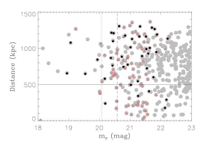
Figure 14: Distance to the group center vs SExtractor r-band magnitude for all galaxies (grey circles). We have also overplotted cluster members (red triangles) and non-cluster members (black circles). The horizontal line shows 500 kpc distance from the galaxy group center (the distance used in the “fossil group” definition). The vertical dotted and dashed lines show $\Delta m_{12}=2.0$ and $\Delta m_{14}=2.5$ respectively, taking $m_{r,SEx}$ as the BGG magnitude.

7.3 The dynamical state of the cluster

The presence of a large magnitude gap has been always taken as indication of relaxed and early-formed galaxy systems. Nevertheless, in the Millennium Simulation can be seen that most of the early-formed systems do not show large magnitude gaps (see Dariush et al. dariush10 (2010)). Thus, overcoming the empirical definitions of “fossil group”, one should consider whether RX J105453.3+552102 is or is not an old and undisturbed system that has underegone little infall of $L^{*}$ galaxies since its initial collapse.

Recent major mergers with other galaxy systems would yield some observable smoking-guns. The first would be the presence of substructure in RX J105453.3+552102. We have used a battery of different tests in 1D, 2D and 3D to take into account the geometry of a possible cluster merger (Pinkney et al. pin96 (1996)). We found no evidence of substructure. The only possible hint is the peculiar velocity of the BGG galaxy (significant at the $>95\%$ c.l.), which is often connected to evidence of substructure (e.g. Bird bir94 (1994)). However, the velocity of the BGG in the cluster rest frame is only $\sim 300$ km s${}^{-1}\;$and the relative peculiar velocity with respect to the cluster velocity dispersion is 0.3, which is not a particularly large value among clusters (see fig. 2 of Coziol et al. coz09 (2009)). Moreover, RX J105453.3+552102 seems well isolated in the phase-space as show by Fig. 6 (see den Hartog & Katgert den96 (1996) and Aguerri et al. aguerri07 (2007) for other clusters). This supports the idea that RX J105453.3+552102 is far from an important accretion episode. Nevertheless, we have shown that, albeit the overall velocity distribution of the spectroscopical galaxy sample belonging to RX J105453.3+552102 is Gaussian, there is a significant departure from Gaussianity in the outer regions ($R>2^{\prime}$) which we have interpreted as a possible signature of radial anisotropy of the galaxies in the group outskirts. If confirmed in more detailed dynamical analysis, this will represent an interesting piece of information to be added into the fossil group information scenarios (D’Onghia et al. 2005; Sommer-Larsen 2006).

The second signature of an old and undisturbed cluster comes from the BGG itself. In fact, RX J105453.3+552102 BGG shows a small $n$ Sérsic index value ($n\approx 2$) and clear discy isophotes in the external regions. According to the findings of numerical simulations, surface brightness profiles with small $n$ values result from gas rich mergers (e.g., Khochfar & Burkert kho05 (2005)). If the RX J105453.3+552102 BGG has indeed been formed from the merger of all major galaxies within the inner regions of the system in very early times, then some of these mergers would have been gas–rich. In contrast, the merger between two clusters and the following equal–mass dry mergers of the corresponding dominant ellipticals would produce surface brightness profiles with $n\approx 4$. Another piece of evidence in favour of the above scenario is the absence of multiple nuclei both from our photometric data and from spectroscopic data. I fact, we took three spectra with different slit position angles crossing the BGG nucleus and giving equal $z$ values.

The third, possible piece of evidence that RX J105453.3+552102 is a relaxed old cluster comes from the dip observed in the photometric LF at $M_{r}\sim-19.5$. This dip is more prominent in the LF_phot computed with the galaxies located within 0.5 Mpc radius. Similar bimodality in the LF has also been reported in other relaxed clusters (Yagi et al. yagi02 (2002)) and groups (Hunsberger et al. huns98 (1998), Miles et al. mil04 (2004), Mendes de Oliveira et al. mendes06 (2006)).

We can conclude that although RX J105453.3+552102 do not follow the prescription of a fossil system, is a relaxed and old galaxy cluster with no indication of recent infall of $L^{*}$ galaxies and therefore, it is a genuine FG.

7.4 RX J105453.3+552102 a relaxed and massive system at z$\approx 0.5$

Our analysis indicates that RX J105453.3+552102 is a very massive galaxy cluster already relaxed at z$\approx$0.5. This means that $\approx 6$ Gyr ago this cluster was as massive as the Coma cluster but more dynamically evolved. In a hierarchical structure formation scenario, these very massive, relaxed systems are likely formed at low redshift. In order to understand how common is a cluster like RX J105453.3+552102, we have searched in the Millennium Simulation (Springel et al. springel05 (2005); Boylan-Kolchin et al. boylan09 (2009)) for halos with masses M${}_{200}>1\times 10^{15}h_{70}^{-1}$ M_⊙ located at z$=0.5$. The total number of such halos was only 9 within the volume covered by the Millennium Simulation (having a box of comoving size of 500 $h_{100}^{-1}$ Mpc). We have also computed the magnitude difference between the brightest and the second brightest galaxies located in each of those halos: only 3/9 have $\Delta m_{12}>2$. However, the Millennium Simulation has been carried out using a normalization of the power spectrum with $\sigma_{8}=0.9$. Using instead a lower normalization, $\sigma_{8}=0.8$, in agreement with the most recent CMB and large-scale structure analysis (e.g. Komatsu et al. 2010, and references therein), the number density of such massive clusters at $z=0.5$ drops by about a factor of three. Thus we expect the number of “fossil” clusters at least as massive as RX J105453.3+552102 within the Millennium Simulation volume at $z=0.5$ to be of order unity. Clearly, to decide whether the detection of a relaxed massive cluster like RX J105453.3+552102 should be considered as a rare event for a standard $\Lambda$CDM cosmology, one has to know the volume within which this cluster has been found, i.e. the selection function of the corresponding survey. We postpone the discussion of this issue to a future analysis, which will also be based on a larger statistics of fossil groups/clusters.

[x]cccccccccc Photometric and kinematic properties of the galaxies observed with DOLORES
SDSS Name cz member comments m_r,our $m_{u,SDSS}$ $m_{g,SDSS}$ $m_{r,SDSS}$ $m_{i,SDSS}$ $m_{z,SDSS}$
(km s^-1)
continued.
SDSS Name cz member comments m_r,our $m_{u,SDSS}$ $m_{g,SDSS}$ $m_{r,SDSS}$ $m_{i,SDSS}$ $m_{z,SDSS}$
(km s^-1)
SDSS J105425.15+552103.0 141485 $\pm$ 100 1 E 24.585 22.081 21.063 20.447 20.566
SDSS J105427.11+552247.4 139639 $\pm$ 108 1 NE 23.500 23.080 21.590 20.760 20.060
SDSS J105428.19+552058.0 191053 $\pm$ 130 0 NE 24.220 22.510 21.960 20.810 20.480
SDSS J105428.47+552123.4 139112 $\pm$ 98 1 NE 21.850 22.660 21.750 21.190 20.960
SDSS J105429.56+551955.6 150572 $\pm$ 72 0 NE 21.520 21.330 20.370 19.830 19.420
SDSS J105430.42+552116.5 141276 $\pm$ 56 1 NE 24.700 22.820 21.370 20.290 19.490
SDSS J105431.81+552224.2 139446 $\pm$ 57 1 NE 25.930 23.320 21.430 20.630 20.300
SDSS J105433.07+552345.3 118229 $\pm$ 116 0 NE 23.580 22.490 20.650 19.980 19.570
SDSS J105433.47+552153.9 139997 $\pm$ 134 1 NE 25.690 23.710 21.920 21.680 20.980
SDSS J105433.59+552315.0 139255 $\pm$ 100 1 E 22.140 21.580 20.660 20.330 20.190
SDSS J105434.56+552233.6 138980 $\pm$ 96 1 NE 25.050 22.750 21.240 20.420 19.890
SDSS J105434.76+552052.0 139734 $\pm$ 80 1 NE 20.91 23.060 22.610 20.850 20.050 19.760
SDSS J105435.18+552057.1 139862 $\pm$ 148 1 NE 20.62 26.140 22.500 20.680 19.910 19.460
SDSS J105435.48+551849.1 108230 $\pm$ 162 0 NE 20.84 22.150 21.750 20.630 20.520 20.500
SDSS J105438.24+552217.1 140766 $\pm$ 69 1 NE 21.32 24.930 23.150 21.410 20.690 20.070
SDSS J105438.39+551806.2 115193 $\pm$ 102 0 NE 23.640 22.540 21.500 21.270 21.010
SDSS J105438.83+552019.8 141886 $\pm$ 81 1 E 20.83 22.360 21.610 20.980 20.520 21.000
SDSS J105438.84+552311.4 139216 $\pm$ 100 1 E 21.46 23.030 22.780 21.710 21.310 21.420
SDSS J105439.21+552108.2 139441 $\pm$ 124 1 NE 21.52 26.600 23.460 21.410 20.780 20.450
SDSS J105439.78+552155.3 142896 $\pm$ 106 1 NE 20.49 25.300 22.000 20.840 20.080 19.750
SDSS J105440.08+551840.2 114765 $\pm$ 58 0 NE 19.06 21.230 20.470 19.350 18.900 18.420
SDSS J105440.09+552056.2 139605 $\pm$ 110 1 NE 21.30 24.760 23.280 21.830 21.000 20.820
SDSS J105440.50+552316.0 72992 $\pm$ 100 0 E 21.59 22.780 22.210 21.810 21.590 21.520
SDSS J105440.71+552157.6 143384 $\pm$ 58 1 NE 20.44 25.720 22.210 20.600 19.790 19.230
SDSS J105442.08+551903.3 137694 $\pm$ 66 1 NE 20.93 23.870 22.340 20.960 20.200 19.840
SDSS J105442.56+552022.8 126728 $\pm$ 166 0 NE 21.25 22.860 22.150 21.410 20.960 20.550
SDSS J105442.81+551922.8 139712 $\pm$ 78 1 NE 21.05 25.170 22.690 21.170 20.270 19.760
SDSS J105442.94+552008.4 138861 $\pm$ 66 1 NE 20.38 25.850 22.660 20.740 19.810 19.520
SDSS J105443.61+552026.8 140214 $\pm$ 40 1 NE 20.69 22.570 22.490 20.850 19.980 19.510
SDSS J105444.08+552059.4 140503 $\pm$ 43 1 NE 20.00 26.290 21.850 20.360 19.480 19.100
SDSS J105444.19+552311.9 93821 $\pm$ 120 0 NE 20.78 23.020 21.800 21.010 20.650 20.520
SDSS J105444.90+552211.2 138104 $\pm$ 51 1 NE 20.99 23.280 22.650 21.210 20.530 20.380
SDSS J105445.14+552044.4 139763 $\pm$ 43 1 NE 20.02 21.880 21.370 20.100 19.450 19.120
SDSS J105445.26+552422.2 125001 $\pm$ 164 0 NE 22.620 22.150 21.260 20.790 20.630
SDSS J105445.51+552005.6 140125 $\pm$ 84 1 NE 21.36 24.730 23.180 21.550 20.750 20.290
SDSS J105445.53+552233.3 137294 $\pm$ 100 1 E 21.57 23.650 21.970 20.290 19.430 19.050
SDSS J105446.25+552231.8 138849 $\pm$ 70 1 NE 20.09 23.650 21.970 20.290 19.430 19.050
SDSS J105446.34+551919.6 129031 $\pm$ 100 0 E 21.54 23.350 22.880 21.650 21.130 20.760
SDSS J105446.60+552400.7 139962 $\pm$ 58 1 NE 21.35 24.710 23.280 21.390 20.400 19.960
SDSS J105446.82+552104.1 139224 $\pm$ 82 1 NE 21.26 23.040 23.070 21.430 20.510 20.310
SDSS J105447.04+551825.6 129392 $\pm$ 80 0 NE 24.850 22.920 20.950 20.460 19.890
SDSS J105447.26+552340.4 139079 $\pm$ 92 1 NE 20.17 26.700 22.080 20.420 19.530 19.280
SDSS J105447.65+552140.4 140759 $\pm$ 94 1 NE 21.50 24.300 23.160 21.770 20.910 20.420
SDSS J105447.87+552111.4 136842 $\pm$ 70 1 NE 21.39 23.480 22.860 21.650 20.880 20.360
SDSS J105448.05+552105.8 139333 $\pm$ 110 1 NE 20.87 26.270 23.230 21.210 20.180 20.010
SDSS J105448.49+552106.3 232784 $\pm$ 100 0 E 22.13 23.670 22.970 22.240 21.750 21.030
SDSS J105448.29+552129.1 140102 $\pm$ 68 1 NE 21.09 24.710 23.370 21.440 20.380 20.300
SDSS J105448.78+551757.0 144715 $\pm$ 100 0 E 22.590 22.470 21.450 21.260 21.270
SDSS J105449.61+552148.0 142630 $\pm$ 96 1 NE 21.55 23.440 23.610 21.580 20.700 20.090
SDSS J105449.69+551921.9 102091 $\pm$ 112 0 NE 18.94 21.760 20.510 19.150 18.590 18.230
SDSS J105449.71+552006.4 114798 $\pm$ 152 0 NE 21.61 25.430 23.070 21.780 21.050 20.920
SDSS J105450.31+552117.3 137712 $\pm$ 70 1 NE 21.04 23.160 22.420 20.930 20.470 19.970
SDSS J105450.37+552229.2 139167 $\pm$ 92 1 NE 20.55 24.430 22.400 20.620 19.720 19.300
SDSS J105451.15+551822.7 110305 $\pm$ 100 0 E 23.630 23.130 21.530 21.090 20.950
SDSS J105451.20+552205.5 137511 $\pm$ 128 1 NE 20.97 23.530 22.710 21.080 20.160 19.990
SDSS J105451.56+552036.4 138463 $\pm$ 182 1 NE 21.25 24.870 22.890 21.200 20.520 20.200
SDSS J105451.93+552058.8 140795 $\pm$ 84 1 NE 21.46 24.470 23.200 21.620 21.560 20.560
SDSS J105452.17+552127.1 140812 $\pm$ 120 1 NE 21.56 25.770 23.360 21.570 20.630 20.140
SDSS J105452.03+552112.5 140223 $\pm$ 39 1 NE 18.08 21.430 19.450 17.690 16.780 16.340
SDSS J105452.57+552111.6 137879 $\pm$ 90 1 NE 21.42 25.110 23.210 22.190 21.190 20.910
SDSS J105452.80+552426.3 194294 $\pm$ 100 0 E 24.150 23.010 21.970 21.550 21.830
SDSS J105452.97+551732.7 115124 $\pm$ 100 0 E 23.350 21.910 21.070 20.700 20.240
SDSS J105453.22+551747.6 140330 $\pm$ 122 1 NE 25.960 23.090 21.200 20.260 19.900
SDSS J105453.25+551911.8 141601 $\pm$ 52 1 NE 20.45 23.290 22.190 20.790 19.930 19.530
SDSS J105453.81+552122.6 141516 $\pm$ 70 1 NE 20.88 25.020 23.030 21.110 20.060 19.710
SDSS J105453.92+552207.9 75671 $\pm$ 150 0 NE 21.26 22.540 22.890 21.350 21.000 20.840
SDSS J105454.00+552129.2 144198 $\pm$ 112 1 NE 21.51 25.740 23.220 21.370 20.710 20.090
SDSS J105454.06+552055.2 140987 $\pm$ 132 1 NE 21.47 25.630 23.330 21.380 20.430 20.050
SDSS J105454.37+552322.4 63639 $\pm$ 100 0 E 20.43 21.940 21.260 20.640 20.220 20.440
SDSS J105454.43+552332.2 139934 $\pm$ 108 1 NE 21.42 25.010 22.940 21.550 21.000 20.250
SDSS J105454.44+552256.2 140911 $\pm$ 50 1 NE 21.09 25.000 22.870 20.870 20.230 19.770
SDSS J105454.52+552153.2 140719 $\pm$ 116 1 NE 20.56 21.630 21.510 20.790 20.570 20.220
SDSS J105454.57+552316.1 138810 $\pm$ 88 1 NE 20.82 24.410 22.170 21.090 20.600 20.040
SDSS J105455.24+552348.7 140494 $\pm$ 84 1 NE 20.56 24.120 22.740 20.830 19.920 19.410
SDSS J105455.24+552229.6 139666 $\pm$ 96 1 NE 21.40 24.140 22.860 21.600 20.910 20.290
SDSS J105455.35+552106.4 139288 $\pm$ 72 1 NE 20.55 23.070 22.410 20.630 19.750 19.350
SDSS J105456.23+552132.3 54707 $\pm$ 100 0 E 20.19 22.870 20.970 20.440 20.220 20.360
SDSS J105456.24+552119.5 138061 $\pm$ 53 1 NE 20.94 25.630 22.860 21.300 20.350 19.970
SDSS J105456.36+551938.0 97145 $\pm$ 100 0 E 21.76 22.310 22.920 21.990 22.070 21.280
SDSS J105456.47+552106.1 138140 $\pm$ 180 1 NE 21.18 24.860 22.730 21.600 20.820 20.390
SDSS J105456.63+552252.9 137620 $\pm$ 97 1 NE 20.48 25.940 22.450 20.550 19.820 19.370
SDSS J105456.65+551850.3 115040 $\pm$ 74 0 NE 20.37 25.200 22.260 20.590 20.000 19.600
SDSS J105456.67+552056.2 140402 $\pm$ 112 1 NE 21.43 22.840 23.030 21.820 20.900 20.520
SDSS J105456.70+552100.2 140377 $\pm$ 86 1 NE 21.25 25.780 22.950 21.540 20.740 20.250
SDSS J105457.29+552132.0 225652 $\pm$ 71 0 E 22.18 24.970 22.570 21.580 20.860 20.640
SDSS J105458.04+552004.3 75840 $\pm$ 100 0 E 21.02 23.350 21.770 20.980 20.910 21.540
SDSS J105459.02+552059.6 141759 $\pm$ 79 1 NE 21.84 24.570 23.140 21.980 21.070 21.120
SDSS J105459.80+551943.5 98567 $\pm$ 120 0 NE 19.54 21.540 20.710 19.750 19.320 19.140
SDSS J105502.36+552222.5 138289 $\pm$ 66 1 NE 20.40 22.720 22.190 20.760 19.930 19.530
SDSS J105502.56+552428.4 145237 $\pm$ 100 0 E 22.570 22.710 21.540 20.950 20.760
SDSS J105502.82+552301.6 93992 $\pm$ 66 0 NE 19.93 23.220 21.350 20.060 19.440 19.020
SDSS J105502.88+552145.9 185676 $\pm$ 100 0 E 20.17 22.150 21.330 20.340 19.540 19.240
SDSS J105503.17+551941.3 147211 $\pm$ 98 0 NE 20.92 23.660 22.430 20.970 20.240 19.830
SDSS J105503.87+552154.0 142410 $\pm$ 82 1 NE 20.52 24.330 22.550 20.920 20.140 19.700
SDSS J105503.87+552108.5 139865 $\pm$ 60 1 NE 20.99 24.640 22.980 21.320 20.530 20.040
SDSS J105504.35+551923.6 146988 $\pm$ 100 0 E 21.39 22.590 22.620 21.880 21.370 21.290
SDSS J105505.49+552034.1 141445 $\pm$ 98 1 NE 21.10 26.610 22.580 21.290 20.680 19.880
SDSS J105505.57+552245.3 139111 $\pm$ 122 1 NE 20.91 23.230 22.130 20.900 20.550 20.070
SDSS J105506.15+551914.6 191048 $\pm$ 100 0 E 21.53 22.800 22.510 21.650 21.490 21.430
SDSS J105506.18+551858.4 137366 $\pm$ 100 1 E 20.04 22.220 21.300 20.260 19.730 19.280
SDSS J105506.23+552257.7 126848 $\pm$ 71 0 E 21.85 23.730 22.760 21.980 22.100 21.200
SDSS J105506.84+552306.3 140352 $\pm$ 138 1 NE 22.15 24.770 23.460 21.960 21.410 20.630
SDSS J105508.66+552121.8 141913 $\pm$ 88 1 NE 20.78 24.170 22.780 21.100 20.440 20.190
SDSS J105509.72+552102.0 107957 $\pm$ 59 0 NE 20.73 22.520 22.060 20.970 20.370 20.020
SDSS J105510.66+552253.3 108052 $\pm$ 100 0 NE 20.44 23.200 22.110 20.690 20.090 19.740
SDSS J105510.89+552323.3 138834 $\pm$ 166 1 NE 21.08 26.460 23.090 21.160 20.260 20.000
SDSS J105511.18+552255.8 75742 $\pm$ 100 0 E 22.810 21.570 20.970 20.640 20.260
SDSS J105511.57+552100.4 140472 $\pm$ 96 1 NE 22.600 21.570 20.790 20.490 20.220
SDSS J105513.08+552315.2 138920 $\pm$ 68 1 NE 24.760 22.630 20.810 20.010 19.400
SDSS J105513.63+552103.5 139550 $\pm$ 84 1 NE 23.940 22.930 21.330 20.570 20.130
SDSS J105514.05+551952.9 190991 $\pm$ 66 0 NE 22.010 21.420 20.460 19.840 19.610
SDSS J105515.13+552058.8 139317 $\pm$ 108 1 NE 23.470 22.990 21.970 21.320 21.040
SDSS J105515.94+552058.7 138504 $\pm$ 156 1 NE 22.850 23.190 21.630 21.000 20.300
SDSS J105516.06+551945.9 139489 $\pm$ 84 1 NE 22.510 21.850 20.970 20.500 20.150
SDSS J105516.15+552030.8 140092 $\pm$ 150 1 NE 24.500 22.680 21.090 20.230 19.870
SDSS J105517.30+552108.0 139511 $\pm$ 70 1 NE 22.280 20.840 19.150 18.340 17.880