Mapping Between Generalized Nonlinear Schrödinger Equations and Neutral Scalar Field Theories and New Solutions of the Cubic-Quintic NLS Equation

Abstract:

We highlight an interesting mapping between the moving breather solutions of the generalized Nonlinear Schrodinger (NLS) equations and the static solutions of neutral scalar field theories. Using this connection, we then obtain several new moving breather solutions of the cubic-quintic NLS equation both with and without uniform phase in space. The stability of some stationary solutions is investigated numerically and the results confirmed via dynamical evolution.

1 Introduction

The nonlinear Schrödinger equation is one of the most celebrated integrable nonlinear equation which has found application in several areas of physics including the self-focusing of intense Laser beams, Langmuir waves in Plasma, the collapse of the Bose-Einstein condensates (BECs) with attractive interactions etc [1]. While most of the applications so far are those of NLS with cubic nonlinearity, in recent years the cubic-quintic NLS (CQNLS) has also found several applications. Some of these are in nonlinear optics and BEC. For example, in nonlinear optics, it describes the propagation of pulses in double-doped optical fibres [2] and in Bragg-gratings [3]; in BEC it models the condensate with two- and three-body interactions [4, 5]. It is thus of considerable interest to obtain exact solutions of the CQNLS and other generalized NLS equations.

In particular, a considerable amount of attention has been given in the recent decades to localized solutions of various NLS, although these solutions exist as the hyperbolic limit of appropriate general elliptic function solutions. This direction has been explored in the context of an external periodic potential [6] as well as weakly interacting solitary waves in generalized NLS equations [7]. Herein we explore exhaustively the analytic elliptic function solutions in the absence of an external potential.

In this context it is worth noting the connection between the moving breather solutions of the generalized NLS equations and the (static) solutions of neutral scalar field theories, known as Galilean invariance. Consider the generalized NLS equation

$$iu_{t}+u_{zz}+f(|u|^{2})u=0\,,$$ (1)

where $f(.)$ is a real valued algebraic function with $f(0)=0$. On using the ansatz

$$u(z,t)=\phi(z-vt-z_{0})\exp{\{(i/2)v(z-kt-\delta)\}}\,,$$ (2)

where $k=(v^{2}+4a)/2v$, it is easily shown that $u$ satisfies Eq. (1) provided $\phi(x)$ satisfies the equation

$$\phi_{xx}+f(\phi^{2})\phi+a\phi=0\,,~{}~{}x=z-vt-z_{0}\,,$$ (3)

which is the static field equation for a scalar field theory with nonlinear interaction term $f(\phi^{2})\phi$. This is a travelling wave solution, and can also be posed in $x$ coordinates by the transformation $\partial_{z}\rightarrow\partial_{x}$ and $\partial_{t}\rightarrow-v\partial_{x}+\partial_{t}$, in which case, considering $z_{0}=0,\delta=0$ without any loss of generality, Eq. (2) can be considered separable in this frame as

$$u(x,t)=\phi(x)\exp{\{(i/2)vx\}}\exp{\{(i/2)(v^{2}-4a)t\}}=\tilde{\phi}(x)\exp{\{-i\tilde{a}t\}}\,.$$ (4)

Now this Galilean transformed solution is a stationary solution in the traveling frame. Actually, we can slightly generalize the above ansatz, i.e. consider instead

$$u(z,t)=\phi(z-vt-z_{0})\exp{\{(i/2)(vz-vkt-\delta+\eta(x))\}}\,,~{}~{}x=z-vt-z_{0}\,.$$ (5)

On equating real and imaginary parts, it is easily shown that, given $g$, if

$$\eta(x)=g\int_{0}^{x}\frac{dx^{\prime}}{\phi^{2}(x^{\prime})}\,,$$ (6)

and

$$\phi_{xx}+f(\phi^{2})\phi+a\phi=\frac{g^{2}}{4\phi^{3}}\,,~{}~{}x=z-vt-z_{0}\,,$$ (7)

with $4a=v(2k-v)$ as above, then (7) solves (1). (Note in the traveling frame of $x$ there would also be an extra nonlinear term due to the first derivative, for $v\neq 0$.)

It thus follows from here that knowing the various static solutions of the scalar field theory (3) or (7), one can immediately write down the moving breather solutions of the corresponding NLS model by using Eqs. (1) and (2). Note that the breather solution of the corresponding NLS model will be uniquely characterized by its five parameters: $v,a,g,\delta$ and $z_{0}$. In particular it follows from here that in order to obtain the breather solutions of the CQNLS equation, which is characterized by

$$f(|u|^{2})=b|u|^{2}+c|u|^{4}\,,$$ (8)

one needs to obtain the static solutions of the $\phi^{2}$-$\phi^{4}$-$\phi^{6}$ field theory characterized by

$$\phi_{xx}+a\phi+b\phi^{3}+c\phi^{5}=0\,,$$ (9)

in case $g=0$ while if $g\neq 0$, then one needs to obtain the solutions of the equation

$$\phi_{xx}+a\phi+b\phi^{3}+c\phi^{5}-\frac{g^{2}}{4\phi^{3}}=0\,.$$ (10)

Note that in the special case of $c=0$, one gets the well known mapping between the celebrated (cubic) NLS and $\phi^{2}$-$\phi^{4}$ field theory. If instead one wants to obtain the breather solutions of the quadratic-cubic NLS characterized by

$$f(|u|^{2})=b|u|+c|u|^{2}\,,$$ (11)

then one needs to obtain the static solutions of the $\phi^{2}$-$\phi^{3}$-$\phi^{4}$ field theory characterized by

$$\phi_{xx}+a\phi+b\phi^{2}+c\phi^{3}=0\,.$$ (12)

We have thus transformed the problem of finding the breather solutions of the generalized NLS models to that of finding static solutions of neutral scalar field theories with power law potentials. There is however, one important difference. In view of the fact that the potential must be bounded from below, in neutral scalar field theory models, normally one takes the coefficient of the leading term in the potential to be positive, i.e. in Eqs. (9) and (12), one takes the coefficient $c<0$. However, in the context of the generalized NLS equations, this coefficient need not necessarily be negative. In fact usually it is taken to be positive, yielding bright solitons while if it is negative, then one obtains dark solitons. It is easily seen that taking the coefficient $c>0$ in Eqs. (9) and (12) is equivalent to considering the solutions of the nonlinear oscillator problem (rather than the field theory problem).

The purpose of this paper is to give exhaustive solutions to the CQNLS as well as quadratic-cubic NLS equation as given by Eq. (12). For that purpose we make use of the known static solutions of the corresponding $\phi^{2}$-$\phi^{4}$-$\phi^{6}$ as well as $\phi^{2}$-$\phi^{3}$-$\phi^{4}$ field theory as well as oscillator models and also obtain few new solutions, which to the best of our knowledge, had not been explicitly written down before in the literature. Further, we also obtain static solutions of the field theory $\phi^{2}$-$\phi^{4}$-$\phi^{6}$-$\phi^{-2}$. In this context, it is worth pointing out that recently we have obtained several static solutions of the coupled $\phi^{2}$-$\phi^{4}$-$\phi^{6}$ [8], $\phi^{2}$-$\phi^{3}$-$\phi^{4}$ [9] as well as $\phi^{2}$-$\phi^{4}$ [10] models from where we can immediately obtain the solutions in the decoupled case, for $c<0$. Extending these ideas, we also obtain solutions of these models even in case $c>0$.

The paper is organized as follows. In Sec. 2 we obtain static solutions of the constant (or linear in the case $v\neq 0$) phase CQNLS problem (i.e. when $\phi^{-2}$ term is absent). In section 2.2 we investigate the linear stability of some of these solutions numerically. In particular, we focus on the hyperbolic limit in which our results here are consistent with the well-known Vakhitov-Kolokolov criterion [11] as well as earlier results for a more general non-linearity [12, 13]. Dynamical evolution confirms the stability results and a connection is observed between the nature of the nonlinearity and the behavior of the unstable evolution. In particular, in the case $c>0$, when $b\leq 0$ the solutions tend to blow-up with a self-similar behavior, while unstable solutions for which $b>0$ do not (perturbations are additive). Then, in Sec. 3 we provide solutions for the $\phi^{2}-\phi^{4}-\phi^{6}-\phi^{-2}$ model as given by Eq. (9) in case each of $a,b,c$ can be either positive or negative. In Appendix A we provide static solutions for the $\phi^{2}-\phi^{3}-\phi^{4}$ model as given by Eq. (12) in case each of $a,b,c$ can be either positive or negative. These will be relevant in the context of the breather solutions of quadratic-cubic NLS. For completeness, in Appendix B we also provide static solutions for the $\phi^{2}-\phi^{4}$ model as given by Eq. (11) in case each of $a,c$ can be either positive or negative. These will be relevant in the context of the breather solutions of NLS. Finally, in Sec. 4 we summarize the results and indicate possible relevance of these results.

2 Solutions of $\phi^{2}$-$\phi^{4}$-$\phi^{6}$ and hence CQNLS Model

2.1 Theoretical development

Let us consider solutions of field Eq. (9). As explained above, once these solutions are obtained, then the solution of the CQNLS equation are immediately obtained from here by using Eqs. (1), (2) and (8). We list below eight distinct periodic solutions to the field Eq. (9), i.e. the trivial phase case of $g=0$. In each case, we also mention the values of the parameters $a,b,c$, in particular, if they are positive or negative.

2.1.1 Dark soliton families

Solution I

It is easily shown [8] that

$$\phi=A\sqrt{1+{\rm sn}(Bx+x_{0},m)}\,,$$ (13)

is an exact solution to the field Eq. (9) provided

$$(5m-1)B^{2}=-4a\,,~{}~{}(5m-1)A^{2}=-\frac{8ma}{b}\,,~{}~{}3(5m-1)b^{2}=64mac\,.$$ (14)

Thus this solution is valid provided $b>0,c<0$ while $a>(<$ or $=)\,0$ depending on if $m<(>$ or $=)\,1/5$. Here ${\rm sn}(x,m)$ and ${\rm cn}(x,m)$, ${\rm dn}(x,m)$ denote Jacobi elliptic functions with modulus $m$ [14, 15].

In the limit $m=1$ the periodic solution (13) goes over to the dark soliton solution

$$\phi=A\sqrt{1+\tanh(Bx+x_{0})}\,,$$ (15)

provided

$$B^{2}=-a\,,~{}~{}A^{2}=-(2a/b)\,,~{}~{}b^{2}=(16/3)ac\,.$$ (16)

Thus the dark soliton solution exists to field Eq. (9) provided $a<0,b>0,c<0$.

Solution II

It is easily shown [8] that

$$\phi=\frac{A{\rm sn}(Bx+x_{0},m)}{\sqrt{1-D{\rm sn}^{2}(Bx+x_{0},m)}}\,,$$ (17)

is an exact solution to the field Eq. (9) provided

$$[3D-(1+m)]B^{2}=-a\,,~{}~{}bA^{2}=2[2D(1+m)-m-3D^{2}]B^{2}\,,$$

$$\frac{3b^{2}}{4ac}=\frac{[2D(1+m)-m-3D^{2}]^{2}}{D(1-D)(m-D)[3D-(1+m)]}\,.$$ (18)

There are different constraints depending on the value of $D$. For example if $D<0$, then this solution is valid provided $a>0,b<0,c>0$. On the other hand, if $D>0$ then while the solution is only valid if $c<0$, the signs of $a,b$ depend on the value of $D$. For example, while $a<(>$ or $=)\,0$ depending on if $D>(<$ or $=)\,(1+m)/3$, $b<(>$ or $=)\,0$ depending on if $D<(>$ or $=)\,\frac{1+m-\sqrt{1-m+m^{2}}}{3}$. Summarizing

$$0<D<\frac{1+m-\sqrt{1-m+m^{2}}}{3}\,,~{}~{}~{}a>0,b<0,c<0\,,$$

$$\frac{1+m-\sqrt{1-m+m^{2}}}{3}<D<\frac{1+m}{3}\,,~{}~{}~{}a>0,b>0,c<0\,,$$

$$\frac{1+m}{3}<D<m\,,~{}~{}~{}a<0,b>0,c<0\,,$$

$$D<0\,,~{}~{}~{}a>0,b<0,c>0\,.$$ (19)

In the limit $m=1$ the periodic solution (17) goes over to the dark soliton solution

$$\phi=\frac{A\tanh(Bx+x_{0})}{\sqrt{1-D\tanh^{2}(Bx+x_{0})}}\,,$$ (20)

provided

$$(3D-2)B^{2}=-a\,,~{}~{}bA^{2}=2(3D-1)(1-D)B^{2}\,,~{}~{}\frac{3b^{2}}{4ac}=\frac{(3D-1)^{2}}{D(3D-2)}\,.$$ (21)

Thus the dark soliton solution exists to field Eq. (9) provided the following constraints are satisfied

$$0<D<\frac{1}{3}\,,~{}~{}~{}a>0,b<0,c<0\,,$$

$$\frac{1}{3}<D<\frac{2}{3}\,,~{}~{}~{}a>0,b>0,c<0\,,$$

$$\frac{2}{3}<D<1\,,~{}~{}~{}a<0,b>0,c<0\,,$$

$$D<0\,,~{}~{}~{}a>0,b<0,c>0\,.$$ (22)

Solution III

It is easily shown [8] that

$$\phi=\frac{A}{\sqrt{1-D{\rm sn}^{2}(Bx+x_{0},m)}}\,,$$ (23)

is an exact solution to the field Eq. (9) provided

$$[3m-(1+m)D]B^{2}=-aD\,,~{}~{}DbA^{2}=2[D^{2}-2D(1+m)+3m]B^{2}\,,$$

$$\frac{3b^{2}}{4ac}=\frac{[D^{2}-2D(1+m)+3m]^{2}}{(1-D)(m-D)[3m-(1+m)D]}\,.$$ (24)

There are different constraints depending on the value of $D$. For example if $D<0$, then this solution is valid provided $a>0,b<0,c>0$. On the other hand, if $D>0$ then while the solution is only valid if $c<0$, the signs of $a,b$ depend on the value of $D$. For example, while $a<0$ in case $m\geq 1/2$, for $m<1/2$, $a<(>$ or $=)\,0$ depending on if $D<(>$ or $=)\,\frac{3m}{(1+m)}$. On the other hand, $b>(<$ or $=)\,0$ depending on if $D<(>$ or $=)\,1+m-\sqrt{1-m+m^{2}}$.

In the limit $m=1$ the periodic solution (23) goes over to the dark soliton solution

$$\phi=\frac{A}{\sqrt{1-D\tanh^{2}(Bx+x_{0})}}\,,$$ (25)

provided

$$(3-2D)B^{2}=-aD\,,~{}~{}DbA^{2}=2(3-D)(1-D)B^{2}\,,~{}~{}\frac{3b^{2}}{4ac}=\frac{(3-D)^{2}}{(3-2D)}\,.$$ (26)

There are different constraints depending on the value of $D$. For example if $D<0$, then this solution is valid provided $a>0,b<0,c>0$. On the other hand, if $D>0$ then the solution is only valid if $a<0,b>0,c<0$.

It is worth pointing out that for $D<0$, solution (23) is not an independent solution but rather can be easily derived from the solution (37) below by using well known transformation formulas for Jacobi elliptic functions and making use of the translational invariance of the solutions. However, for $D>0$, (23) is an independent solution.

2.1.2 Bright soliton families

Solution I

It is easily shown that

$$\phi=A\sqrt{1+{\rm cn}(Bx+x_{0},m)}\,,$$ (27)

is an exact solution to the field Eq. (9) provided

$$(4m+1)B^{2}=4a\,,~{}~{}(4m+1)A^{2}=-\frac{8ma}{b}\,,~{}~{}3(4m+1)b^{2}=64mac\,.$$ (28)

Thus this solution is valid provided $a>0,b<0,c>0$.

In the limit $m=1$ the periodic solution (27) goes over to the bright soliton solution

$$\phi=A\sqrt{1+{\rm sech}(Bx+x_{0})}\,,$$ (29)

provided

$$5B^{2}=4a\,,~{}~{}5A^{2}=-(8a/b)\,,~{}~{}15b^{2}=64ac\,.$$ (30)

Thus the bright soliton solution exists to field Eq. (9) provided $a>0,b<0,c>0$.

Solution II.1

It is easily shown that

$$\phi=A\sqrt{1+{\rm dn}(Bx+x_{0},m)}\,,$$ (31)

is an exact solution to the field Eq. (9) provided

$$(4+m)B^{2}=4a\,,~{}~{}(4+m)A^{2}=-\frac{8a}{b}\,,~{}~{}3(4+m)b^{2}=64ac\,.$$ (32)

Thus this solution is valid provided $a>0,b<0,c>0$.

In the limit $m=1$ the periodic solution (31) goes over to the bright soliton solution (29) satisfying the constraints (30).

Solution II.2

It is easily shown that

$$\phi=A\sqrt{{\rm dn}(Bx+x_{0},m)+k^{\prime}}\,,~{}~{}k^{\prime}=\sqrt{1-m}\,,$$ (33)

is an exact solution to the field Eq. (9) provided

$$(4-5m)B^{2}=4a\,,~{}~{}bA^{2}=-2B^{2}k^{\prime}\,,~{}~{}cA^{4}=(3/4)B^{2}\,.$$ (34)

Thus this solution is valid provided $b<0,c>0$ while $a>(<$ or $=)\,0$ depending on if $m<(>$ or $=)\,(4/5)$. .

In the limit $m=1$ the periodic solution (33) goes over to the bright soliton solution

$$\phi=A\sqrt{{\rm sech}(Bx+x_{0})}\,,$$ (35)

provided

$$B^{2}=-4a\,,~{}~{}b=0\,,~{}~{}cA^{4}=(3/4)B^{2}\,.$$ (36)

Thus the bright soliton solution exists to field Eq. (9) provided $a<0,b=0,c>0$.

Solution II.3

It is easily shown that

$$\phi=A\sqrt{{\rm dn}(Bx+x_{0},m)-k^{\prime}}\,,~{}~{}k^{\prime}=\sqrt{1-m}\,,$$ (37)

is an exact solution to the field Eq. (9) provided

$$(4-5m)B^{2}=4a\,,~{}~{}bA^{2}=2B^{2}k^{\prime}\,,~{}~{}cA^{4}=(3/4)B^{2}\,.$$ (38)

Thus this solution is valid provided $b>0,c>0$ while $a>(<$ or $=)\,0$ depending on if $m<(>$ or $=)\,(4/5)$. .

In the limit $m=1$ the periodic solution (37) goes over to the bright soliton solution (35) satisfying the constraints (36).

Solution III

It is easily shown [8] that

$$\phi=\frac{A{\rm cn}(Bx+x_{0},m)}{\sqrt{1-D{\rm sn}^{2}(Bx+x_{0},m)}}\,,$$ (39)

is an exact solution to the field Eq. (9) provided

$$[2m-1-D(2-m)]B^{2}=-(1-D)a\,,~{}~{}(1-D)bA^{2}=2[(1+2D)m-D(D+2)]B^{2}\,,$$

$$\frac{3b^{2}}{4ac}=\frac{[(1+2D)m-D(D+2)]^{2}}{D(m-D)[2m-1-D(2-m)]}\,.$$ (40)

There are different constraints depending on the value of $D$. For example if $D<0$, then this solution is valid provided $c>0$. On the other hand, the signs of $a,b$ depend on the value of $D<0$. For example, while for $m\geq 1/2$, $a<0$, for $m<1/2$, $a>(<$ or $=)\,0$ depending on if $|D|<(>$ or $=)\,\frac{1-2m}{2-m}$. On the other hand $b>(<$ or $=)\,0$ provided $|D|<(>$ or $=)\,1-m+\sqrt{1-m+m^{2}}$.

On the other hand, if $0<D<m$, then this solution is valid if $c<0$, while the signs of $a,b$ depend on the value of $D>0$. In particular, while $a>0$ in case $m\leq 1/2$, for $m>1/2$, $a<0$ in case $0<D<\frac{2m-1}{2-m}$ while $a>0$ provided $\frac{2m-1}{2-m}<D<m$. On the other hand, $b>0$ if $0<D<-(1+m)+\sqrt{1-m+m^{2}}$, $b<0$ in case $-(1+m)+\sqrt{1-m+m^{2}}<D<m$.

In the limit $m=1$ the periodic solution (39) goes over to the bright soliton solution

$$\phi=\frac{A{\rm sech}(Bx+x_{0})}{\sqrt{1-D\tanh^{2}(Bx+x_{0})}}\,,$$ (41)

provided

$$B^{2}=-a\,,~{}~{}bA^{2}=2(1+D)B^{2}\,,~{}~{}\frac{3b^{2}}{4ac}=\frac{(1+D)^{2}}{D}\,.$$ (42)

Thus the bright soliton solution exists to field Eq. (9) provided the following constraints are satisfied

$$0<D<1\,,~{}~{}~{}a<0,b>0,c<0\,,$$

$$-1<D<0\,,~{}~{}~{}a<0,b>0,c>0\,,$$

$$D<-1\,,~{}~{}~{}a<0,b<0,c>0\,.$$ (43)

Solution IV

It is easily shown [8] that

$$\phi=\frac{A{\rm dn}(Bx+x_{0},m)}{\sqrt{1-D{\rm sn}^{2}(Bx+x_{0},m)}}\,,$$ (44)

is an exact solution to the field Eq. (9) provided

$$[2m-m^{2}-D(2m-1)]B^{2}=-(m-D)a\,,$$

$$(m-D)bA^{2}=2[(1-2D)m-D(D-2)]B^{2}\,,$$

$$\frac{3b^{2}}{4ac}=\frac{[(1-2D)m-D(D-2)]^{2}}{D(1-D)[2m-m^{2}-D(2m-1)]}\,.$$ (45)

There are different constraints depending on the value of $D$. For example if $0<D<m$, then this solution is valid provided $a<0,b>0,c<0$.

On the other hand, if $D<0$, then this solution is valid if $c>0$, while the signs of $a,b$ depend on the value of $D<0$. In particular, while $a<0$ in case $m\geq 1/2$, for $m<1/2$, $a<0$ in case $0<|D|<\frac{m(2-m)}{1-2m}$ while $a>0$ provided $\frac{m(2-m)}{1-2m}<D<m$. On the other hand, $b>0$ if $0<D<-(1-m)+\sqrt{1-m+m^{2}}$ while $b<0$ in case $-(1-m)+\sqrt{1-m+m^{2}}<D<m$.

In the limit $m=1$ the periodic solution (44) goes over to the bright soliton solution (41) satisfying the constraints as given by Eqs. (42) and (2.1.2).

It is worth pointing out that for $D>0$, solution (44) is not an independent solution but rather can be easily derived from the solution (39) by using well known transformation formulas for Jacobi elliptic functions and making use of the translational invariance of the solutions. However, for $D<0$, (44) is an independent solution.

2.2 Numerical Solutions and Stability Analysis

We will now look at some of the particular solutions presented above and investigate their stability properties both through a systematic linear stability analysis and also dynamical evolution. In particular, we consider exhaustively the various regimes of hyperbolic dark and bright soliton solutions with trivial phase from section 2, as well as some elliptic examples from the same section. In considering the structural linearized stability we will consider the static reference frame (i.e. v=0) and focus on the stationary wave solutions. Such stationary solutions have Galilean invariance, yielding the ansatz for the traveling wave given in Eq. (3). Although, assuming a traveling reference frame and Galilean transformations of the perturbations as well, the equations for dynamical stability of static ($v=0$) and traveling wave ($v\neq 0$) solutions are equivalent. We note that above the Landau critical velocity, the solution will be so-called Landau-unstable [16], although this instability is not expected to have any effect in the absence of any external potential, and is usually investigated in the presence of an external impurity [17] or lattice [18].Given a solution $\phi$ of (3), we consider the linearization of Eq. (1) around this stationary solution, i.e. assume the following ansatz, for $\epsilon\ll 1$,

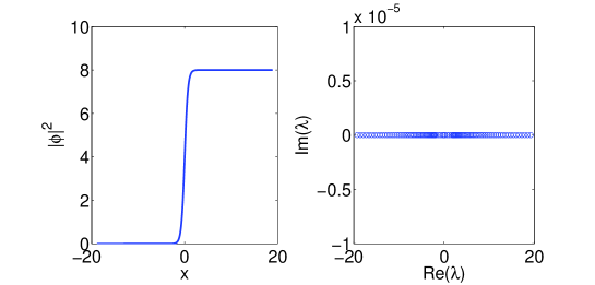
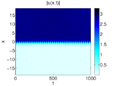
Figure 1: (Color Online) Left: Dark soliton solution I with $m=1,a=-2,b=1$ (left), and the linearization spectrum as computed by Eq. (46). Right: Dynamical evolution of $u=\phi+r$, where $r=p{\rm max}|\phi(x,0)|^{2}U$, $p=0.05$, $U$ is a uniformly distributed random variable in $(0,1)$, and $\phi$ is solution I with $m=1,a=-2,b=1$, as shown to the left. The stability is confirmed as the solution sustains only minor oscillations from its original form after the $5\%$ perturbation.

$$u(z,t)=e^{-iat}[\phi(z)+\epsilon\tilde{u}(z,t)]\,.$$ (46)

Assuming $\tilde{u}=w(x)e^{i\lambda t}$ is separable then we have the following linearization system

$\bordermatrix{&\cr&\mathcal{L}_{1}&\mathcal{L}_{2}\cr&-\mathcal{L}_{2}^{*}&-\mathcal{L}_{1}^{*}\cr}v=\lambda v$

for any arbitrary eigenfunction $v$ (which includes the possibility of a more general spatial form of the perturbations). The blocks are given by

$$\mathcal{L}_{1} = a+\partial_{xx}+2b|\phi|^{2}+3c|\phi|^{4}\,,$$

$$\mathcal{L}_{2} = b\phi^{2}+2c|\phi|^{2}\phi^{2}.$$

This eigenvalue problem, commonly known as the Bogoliubov system, has been solved with both the matlab functions eig in which the full matrix is diagonalized and eigs, which implements the standard ARPACK Arnoldi iterative algorithm to solve for the smallest/largest $n$ eigenvalues. In particular, the latter, quicker and more efficient method for evaluating a particular subset of eigenvalues, is used for exhaustive continuations and benchmarking over much finer spatial grids, while agreement is found in all cases in which both methods are used.

2.2.1 Dark soliton families

For the first family of solutions given by Eqs. (13,15), the hyperbolic tangent [$m=1$, Eq. (15)] (also known as “kink”, or “dark soliton”) solution was found to be stable, just like in the case of the cubic NLS. An example solution is presented in the left panels of Fig. 1 for $a=-2$ and $b=1$. Continuations of these solutions for $(a,b)\in[-2,-.1]\times[.01,1]$ were performed and there was no deviation from this stability result. It seems reasonable to conclude that this is universal, although we did not do an exhaustive search of parameter space. The stability results were then confirmed with dynamical evolution using a standard fourth order Runge-Kutta method. The right panel of Figure (1) displays the result of evolving $u=\phi+r$, where $r=p{\rm max}|\phi(x,0)|^{2}U$, $p=0.05$ and $U$ is a uniformly distributed random variable in $(-1,1)$. Notice even with this large perturbation, the robust structure persists for up to at least $t=1000$, experiencing only minor oscillations around the stationary solution.

It is most likely a result of the fact that the solutions for $m\neq 1$ are “very nearly non-differentiable” that, even with appropriately matched periodic boundary conditions, the norm difference of the exact solution with the one on the numerical grid is orders of magnitude larger than that of the hyperbolic kin. This prevents such a systematic numerical analysis of the stability, although using the exact solution as an initial guess for a fixed point solver on the numerical grid, the solution does converge to a smoother version which is wildly unstable, and this suggests these solutions are unstable.

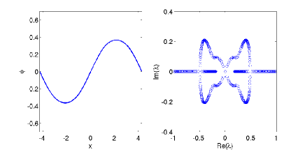
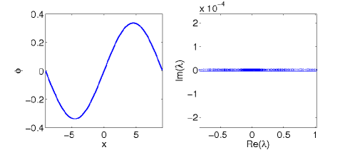
Figure 2: (Color Online) The left two panels show the dark soliton solution II (left) with unstable parameters $(a,b,D,m)=(0.75,1,0.3,0.7)$ and the linearization spectrum is on the right as given by Eqs. (46). The right panels show a solution from the same family but for a set of parameters for which the solution is stable, $(a,b,D,m)=(0.1,0.5,0.3,0.5)$.

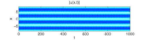
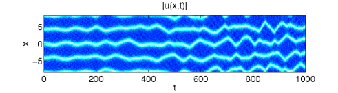
Figure 3: (Color Online) The left panel is the dark soliton solution II with unstable parameters $(a,b,D,m)=(0.75,1,0.3,0.7)$ from the left of Fig. 2, while the right is for the unstable parameters $(a,b,D,m)=(1.5,1.5,0.5,0.99)$.

Next, we consider the smoother family of dark-soliton solutions II given in Eqs. (17,20). For the hyperbolic solutions (m=1), Eq. (20), a representative value of $D$ was chosen for all the intervals defined in Eq. (2.1.1), with the exception of the interval $2/3<D<1$, where the signs of $b$ and $c$ are the same as solution I above. For each of these values of $D\in\{-0.2,0.1,0.35\}$, a two parameter continuation was done for the corresponding values of $(|a|,|b|)\in[.1,1]\times[.01,1]$. All solutions were found to be stable. Some periodic solutions ($m\neq 1$) from this smoother family were also found. For certain parameters, the solutions are actually stable, while for others, they are very unstable. The unstable solution for $(a,b,D,m)=(0.75,1,0.3,0.7)$, and the stable one for $(a,b,D,m)=(0.1,0.5,0.3,0.5)$ as given in Eq. (17), and their linearization spectra are shown in Fig. (2). We note here that the Floquet theorem has been invoked in conjunction with periodic boundary conditions, since the stability matrix of the periodic solution is periodic, in order to scan the infinite energy spectrum with a subdivision of $200$ separate spatial frequencies out of the infinitely many. Notice the continuum of eigenvalues with negative imaginary part which form loops symmetric with respect to both the real and imaginary axes (the symmetry is a result of the fact that the matrix is Hamiltonian). The dynamics of the unstable solution with $(a,b,D,m)=(0.75,1,0.3,0.7)$ from the left panels of Fig. 2 are shown on the left panel of Fig. 3. The linear instability has almost no discernible effect on the evolution even with a very large $25\%$ perturbation of the initial amplitude. Somehow the stability properties of the hyperbolic limit are “inherited” by its family, regardless of stability of the linearized system. This presumably has to do with this solution residing at a small steep local maximum of the energy within a large basin, in which a small perturbation is enough to leave the linear regime, but not to significantly alter the structure of the solution (the unstable eigenfunctions are presumably of a very similar form as the solution). We believe this “non-linear stability” is an interesting phenomenon, but is outside the scope of this paper and will be investigated further elsewhere. The right panel shows the evolution of another unstable solution from this family for parameter values $(a,b,D,m)=(1.5,1.5,0.5,0.99)$, where the instability has a greater effect, but still rather negligible and at long times considering the large perturbation. Many other unstable solutions from this family were evolved with large perturbations and this was the most unstable among them.

2.2.2 Bright soliton families

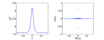
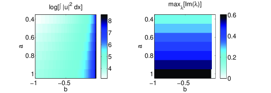
Figure 4: (Color Online) Left panels are the bright soliton solution I with $m=1,a=1,b=-1$ (left), and its linearization spectrum. Right panels depict the power (left, given on a log scale) and stability (right), as indicated by the maximum imaginary part of the spectrum, of a two-parameter family of bright-soliton solutions I (of Eq. (29) with $m=1$ and $(a,b)\in[0.4,1]\times[-0.01,-1]$.

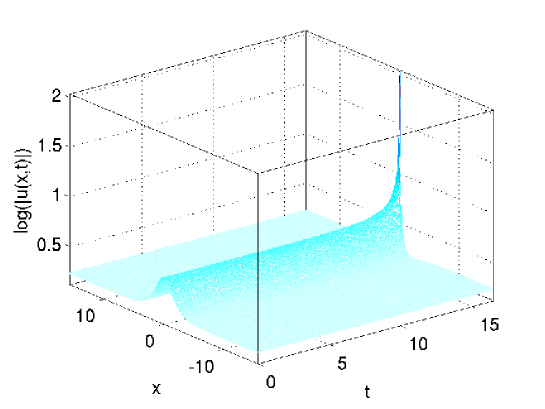
Figure 5: (Color Online) Dynamical evolution of $u=\phi+r$, where $r=p{\rm max}|\phi(x,0)|^{2}U$, $p=0.05$, $U$ is a uniformly distributed random variable in $(0,1)$ and $\phi$ is solution I with $m=1,a=1,b=-1$, as shown if Fig. (4). The stability is confirmed and the solution collapses with exponentially self-similar nature. A $\log$ scale is used for the intensity to illustrate this.

Next we turn to the bright soliton solutions. Now the hyperbolic [$m=1$, Eq. 29] solution (namely “pulse”, “bright soliton”, or just “soliton”) is actually unstable (see, e.g. [12]). This is markedly different from the cubic NLS case, where the analogous solution is stable. This can be connected to the fact that it is well-known that the $H^{1}$ norm (or, energy) of the solution to Eq. (1) for $f(x)=x^{2\sigma}$ is bounded for $\sigma<2/d$, where $d$ is the dimensionality of the problem [13]. The value $\sigma$ is known as the critical exponent, and in our case of $d=1$, we have $\sigma=4$. This is the smallest power nonlinearity for which blowup can occur, corresponding to an exact balance between kinetic and potential energies under the constraint of conserved mass. The solution and its stability are presented in the left panels of Fig. (4). A two-parameter continuation in the parameters $a$ and $b$ (with $c$ determined by them) was performed in order to confirm that the family of solutions is always unstable in the region $(a,b)\in[0.4,1]\times[-1,-0.01]$, as presented in the right panels of Fig. (4). The stability here can also be understood in terms of the Vakhitov-Kolokolov criterion [11], since $dN/da>0$. The small region of stable solutions with very large amplitudes for very small $b$ are actually constant solutions, since for increasing $b$ the amplitude of the soliton shrinks, while the “pedestal” (plane wave) it is sitting on grows. The dynamical evolution given in Fig.(5) confirms the prediction and the solution collapses around $t=15$. The collapse of the waveform is presented on a $\log$ scale so it can be appreciated.

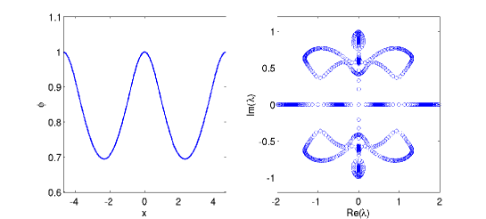
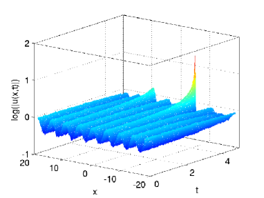
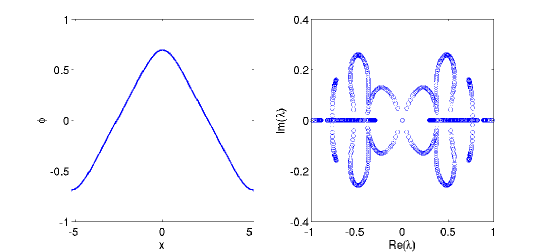
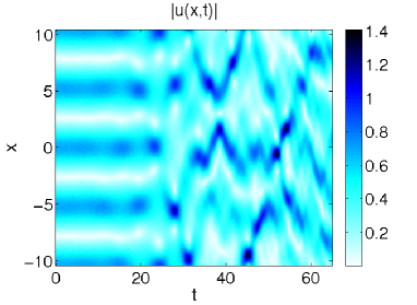
Figure 6: (Color Online) Top: bright soliton solution II.2 with $(a,b,m)=(-0.15,-1,0.9)$, ($c\approx 1.56$). The linearization spectrum is given in the middle as defined in Eqs. (46), and the dynamical evolution is to the right. Bottom: Bright soliton solution III with $(a,b,m,D)=(-0.1,1,0.4,-0.3)$, ($c\approx 0.98$).

It is interesting to note that the instability to collapse appears to be correlated to the sign of the cubic term for the bright solitons (again consistent with the findings of [12]). That is to say, those bright solitons we found for which $b>0$ were stable, while for $b<0$ they were unstable ($c>0$ of course). In particular, we now turn to solutions of Eq. (39). Two parameter continuations were performed for $D\in\{-1.5,-0.3,-0.1,0.1,0.6\}$ and $(|a|,|b|)\in[0.1,1]\times[0.01,1]$, and the last four were invariably stable, for all of which $b>0$ (for the former two $c>0$ and for the latter two $c<0$). For the first value of $D$ the corresponding $b$ is negative (and of course $c>0$) and, as in solution I, the solution is unstable in the entire parameter region. It should be noted that the solution in Eq. (35) where $b=0$ and $c>0$ is linearly stable as the imaginary pair of eigenvalues for $b<0$ pass through the origin and become real for $b<0$. This extra pair of eigenvalues is in addition to one pair associated to phase invariance, $\delta$ in Eq. (2), and one pair associated to translational invariance, $z_{0}$ in Eq. (2), and is due to the conformal invariance of the soliton solution of the critical NLS. This solution is, hence, unstable to collapse as well, despite its linear stability.

Most solutions were found to be unstable, and in fact, no bright soliton family solutions were found that are stable, although in the high-dimensional parameter space among the infinitely many solutions, we by no means discount the possibility that such solutions may exist. As examples we present the solution II.2 for the values $(a,b,m)=(-0.15,-1,0.9)$ as given in Eq. (33) and the solution III for values $(a,b,m,D)=(-0.1,1,0.4,-0.3)$. The solution with $b<0$ [solution II.2, Fig. (6)] does exhibit collapse phenomenon like the unstable soliton, while the one with $b>0$ [solution III] does not.

3 Solutions of $\phi^{2}-\phi^{4}-\phi^{6}-\phi^{-2}$ and hence CQNLS Model

Let us consider solutions of field Eq. (10). As explained above, once these solutions are obtained, then the solution of the CQNLS equation are immediately obtained from here by using Eqs. (1), (5), (6), (7) and (8). We list below five distinct solutions to the field Eq. (10) out of which four are periodic.

Solution I

It is easily shown that

$$\phi=\sqrt{\frac{A{\rm sn}(Gx+x_{0},m)+B}{D{\rm sn}(Gx+x_{0},m)+F}}\,,$$ (47)

is an exact solution to the field Eq. (10) provided the following five coupled equations are satisfied:

$$mG^{2}(AF-BD)(3AF+BD)=g^{2}D^{4}-4A^{2}(aD^{2}+bAD+cA^{2})\,,$$ (48)

$$G^{2}(AF-BD)[2mBF+(1+m)AD]=2g^{2}D^{3}F-4aAD(AF+BD)$$

$$-2bA^{2}(AF+3BD)-8cA^{3}B\,,$$ (49)

$$(1+m)G^{2}(AF-BD)^{2}=-6g^{2}D^{2}F^{2}+4a(A^{2}F^{2}+B^{2}D^{2}+4ABDF)$$

$$+12bAB(AF+BD)+24cA^{2}B^{2}\,,$$ (50)

$$G^{2}(AF-BD)[2AD+(1+m)BF]=-2g^{2}DF^{3}+4aBF(AF+BD)$$

$$+2bB^{2}(3AF+BD)+8cAB^{3}\,,$$ (51)

$$-G^{2}(AF-BD)(AF+3BD)=g^{2}F^{4}-4B^{2}(aF^{2}+bBF+cB^{2})\,.$$ (52)

Thus we have five coupled equations relating the five parameters $A,B,D,G,g$ (note that we can always remove one of the parameter from the ansatz (47)). In the special case of $m=1$, the solution (47) goes over to the hyperbolic soliton solution

$$\phi=\sqrt{\frac{A\tanh(Gx+x_{0})+B}{D\tanh(Gx+x_{0})+F}}\,,$$ (53)

while in the limit $m=0$ it goes over to the trigonometric solution

$$\phi=\sqrt{\frac{A\sin(Gx+x_{0})+B}{D\sin(Gx+x_{0})+F}}\,.$$ (54)

In the special case of $D=0$, $F=1$, we obtain a simpler solution

$$\phi=\sqrt{A{\rm sn}(Gx+x_{0},m)+B}\,,$$ (55)

provided

$$a<0,~{}c<0\,,~{}~{}G^{2}=\frac{9b^{2}-32|a||c|}{8|c|(1+m)}\,,~{}~{}A^{2}=\frac{3mG^{2}}{4|c|}\,,~{}~{}B=\frac{3b}{8|c|}\,,$$ (56)

while $g$ for this solution is given by

$$g^{2}=4B^{2}(a+bB+cB^{2})-A^{2}G^{2}$$

$$=\frac{3}{[32(1+m)]^{2}|c|^{3}}[192b^{2}|a||c|(10m-1-m^{2})$$

$$-(64|a||c|)^{2}m-9b^{4}(26m-5-5m^{2})]\,.$$ (57)

It is easily checked that so long as $g\neq 0$, such a solution does not exist for $m=1$, even though it exists for a range of values of $m<1$. Also note that the solution (55) does not exist in the trigonometric limit of $m=0$ unless $c=0$.

Solution II

Yet another solution to the field Eq. (10) is

$$\phi=\sqrt{\frac{A{\rm cn}(Gx+x_{0},m)+B}{D{\rm cn}(Gx+x_{0},m)+F}}\,,$$ (58)

provided the following five coupled equations are satisfied:

$$mG^{2}(AF-BD)(3AF+BD)=-g^{2}D^{4}+4A^{2}(aD^{2}+bAD+cA^{2})\,,$$ (59)

$$G^{2}(AF-BD)[2mBF+(2m-1)AD]=-2g^{2}D^{3}F$$

$$+4aAD(AF+BD)+2bA^{2}(AF+3BD)+8cA^{3}B\,,$$ (60)

$$(2m-1)G^{2}(AF-BD)^{2}=6g^{2}D^{2}F^{2}-4a(A^{2}F^{2}+B^{2}D^{2}+4ABDF)$$ (61)

$$-12bAB(AF+BD)-24cA^{2}B^{2}\,,$$

$$G^{2}(AF-BD)[2AD(1-m)-(2m-1)BF]=-2g^{2}DF^{3}$$

$$+4aBD(AF+BD)+2bB^{2}(3AF+BD)+8cAB^{3}\,,$$ (62)

$$-(1-m)G^{2}(AF-BD)(AF+3BD)=g^{2}F^{4}-4B^{2}(aF^{2}+bBF+cB^{2})\,.$$ (63)

In the special case of $m=1$, the solution (58) goes over to the hyperbolic soliton solution

$$\phi=\sqrt{\frac{A{\rm sech}(Gx+x_{0})+B}{D{\rm sech}(Gx+x_{0})+F}}\,,$$ (64)

while in the limit $m=0$ it goes over to the trigonometric solution

$$\phi=\sqrt{\frac{A\cos(Gx+x_{0})+B}{D\cos(Gx+x_{0})+F}}\,.$$ (65)

In the special case of $D=0$, $F=1$, we obtain a simpler solution

$$\phi=\sqrt{A{\rm cn}(Gx+x_{0},m)+B}\,,$$ (66)

provided

$$c>0\,,~{}~{}G^{2}=\frac{9b^{2}-32ac}{8c(2m-1)}\,,~{}~{}A^{2}=\frac{3mG^{2}}{4c}\,,B=-\frac{3b}{8c}\,,$$ (67)

while $g$ for this solution is given by

$$g^{2}=4B^{2}(a+bB+cB^{2})-(1-m)A^{2}G^{2}$$

$$=\frac{3}{[32(2m-1)]^{2}c^{3}}[192b^{2}ac(1+8m-8m^{2})$$

$$-(64ac)^{2}m(1-m)-9b^{4}(5+16m-16m^{2})]\,.$$ (68)

Thus unlike solution (47), such a solution always exists in the hyperbolic limit so long as $32ac<9b^{2}<(192/5)ac$. Further, it also exists for a range of values of $m$, though it does not exist in the $m=0$ limit, unless $c=0$.

In the special case of $m=1/2$, we obtain a one-parameter family of solutions of the form (66). In particular, in that case it follows from Eq. (67) that

$$9b^{2}=32ac\,,~{}~{}A^{2}=\frac{3G^{2}}{8c}\,,~{}~{}B=-\frac{3b}{8c}\,,~{}~{}g^{2}=\frac{a^{2}}{3c}-\frac{4cA^{4}}{3}\,.$$ (69)

It is worth noting that while $A,G$ are arbitrary with their ratio being fixed, the only constraint that we have is that $A^{2}<\frac{a}{2c}$ so that $g$ is nonzero and real.

Unlike the ${\rm sn}$ case, in this case solutions exist even in case $A=0$ (and assuming $B=1$ without any loss of generality). In particular,

$$\phi=\frac{1}{\sqrt{D{\rm cn}(Gx+x_{0},m)+F}}\,,$$ (70)

is an exact solution to Eq. (10) provided

$$mG^{2}=g^{2}D^{2}\,,~{}~{}3(1-m)D^{2}G^{2}=g^{2}F^{4}-4(aF^{2}+bF+c)\,,$$

$$(2m-1)G^{2}=2(3g^{2}F^{2}-2a)\,,~{}~{}4g^{2}F^{3}=b+4aF\,.$$ (71)

Note that such a solution exists in the hyperbolic limit ($m=1$) but not in the trigonometric limit ($m=0$).

Solution III

Yet another solution to the field Eq. (10) is

$$\phi=\sqrt{\frac{A{\rm dn}(Gx+x_{0},m)+B}{D{\rm dn}(Gx+x_{0},m)+F}}\,,$$ (72)

provided the following five coupled equations are satisfied:

$$-G^{2}(AF-BD)(3AF+BD)=g^{2}D^{4}-4A^{2}(aD^{2}+bAD+cA^{2})\,,$$ (73)

$$G^{2}(AF-BD)[2BF+(2-m)AD]=-2g^{2}D^{3}F+4aAD(AF+BD)$$ (74)

$$+2bA^{2}(AF+3BD)+8cA^{3}B\,,$$

$$(2-m)G^{2}(AF-BD)^{2}=6g^{2}D^{2}F^{2}-4a(A^{2}F^{2}+B^{2}D^{2}+4ABDF)$$

$$-12bAB(AF+BD)-24cA^{2}B^{2}\,,$$ (75)

$$G^{2}(AF-BD)[2AD(1-m)-(2-m)BF]=-2g^{2}DF^{3}$$

$$+4aBD(AD+BF)+2bB^{2}(3AF+BD)+8cAB^{3}\,,$$ (76)

$$(1-m)G^{2}(AF-BD)(AF+3BD)=g^{2}F^{4}-4B^{2}(aF^{2}+bBF+cB^{2})\,.$$ (77)

In the special case of $m=1$, the solution (72) goes over to the hyperbolic soliton solution (64).

In the special case of $D=0$, $F=1$, we obtain a simpler solution

$$\phi=\sqrt{A{\rm dn}(Gx+x_{0},m)+B}\,,$$ (78)

provided

$$c>0\,,~{}~{}G^{2}=\frac{9b^{2}-32ac}{8c(2-m)}\,,~{}~{}A^{2}=\frac{3G^{2}}{4c}\,,B=-\frac{3b}{8c}\,,$$ (79)

while $g$ for this solution is given by

$$g^{2}=4B^{2}(a+bB+cB^{2})+(1-m)A^{2}G^{2}$$

$$=\frac{3}{[32(2-m)]^{2}c^{3}}[192b^{2}ac(m^{2}+8m-8)$$

$$+(64ac)^{2}(1-m)+9b^{4}(16-16m-5m^{2})]\,.$$ (80)

Like the ${\rm cn}$ case, in this case too solutions exist in case $A=0$ (and assuming $B=1$ without any loss of generality). In particular,

$$\phi=\frac{1}{\sqrt{D{\rm dn}(Gx+x_{0},m)+F}}\,,$$ (81)

is an exact solution to Eq. (10) provided

$$G^{2}=g^{2}D^{2}\,,~{}~{}3(1-m)D^{2}G^{2}=-g^{2}F^{4}+4(aF^{2}+bF+c)\,,$$

$$(2-m)G^{2}=2(3g^{2}F^{2}-2a)\,,~{}~{}4g^{2}F^{3}=b+4aF\,.$$ (82)

Note that this solution is valid for all values of $m$ including the hyperbolic limit of $m=1$.

However, unlike the ${\rm cn}$ case, in this case solution exists even in case $B=0$ (and assuming $A=1$ without any loss of generality). In particular

$$\phi=\sqrt{\frac{{\rm dn}(Gx+x_{0},m)}{D{\rm dn}(Gx+x_{0},m)+F}}\,,$$ (83)

is an exact solution to Eq. (10) provided

$$(1-m)G^{2}=g^{2}F^{2}\,,~{}~{}3F^{2}G^{2}=-g^{2}D^{4}+4(aD^{2}+bD+c)\,,$$

$$(2-m)G^{2}=2(3g^{2}D^{2}-2a)\,,~{}~{}4g^{2}D^{3}=b+4aD\,.$$ (84)

Note that such a solution does not exist in the hyperbolic limit so long as $g\neq 0$.

Solution IV

It is easily shown that

$$\phi=\sqrt{\frac{A{\rm sn}^{2}(Gx+x_{0},m)+B}{D{\rm sn}^{2}(Gx+x_{0},m)+F}}\,,$$ (85)

is an exact solution to the field Eq. (10) provided the following five coupled equations are satisfied:

$$4mG^{2}AD(AF-BD)=-g^{2}D^{4}+4A^{2}(aD^{2}+bAD+cA^{2})\,,$$ (86)

$$G^{2}(AF-BD)[2mAF+2(1+m)AD]=g^{2}D^{3}F-2aAD(AF+BD)$$

$$-bA^{2}(AF+3BD)-4cA^{3}B\,,$$ (87)

$$2G^{2}(AF-BD)[3mBF-(1+m)AF+(1+m)BD-3AD]$$ (88)

$$=3g^{2}D^{2}F^{2}-2a(A^{2}F^{2}+B^{2}D^{2}+4ABDF)$$

$$-6bAB(AF+BD)-12cA^{2}B^{2}\,,$$

$$2G^{2}(AF-BD)B[D+(1+m)F]=-g^{2}DF^{3}+2aBF(AF+BD)$$

$$+bB^{2}(3AF+BD)+4cAB^{3}\,,$$ (89)

$$4G^{2}(AF-BD)BF=g^{2}F^{4}-4B^{2}(aF^{2}+bBF+cB^{2})\,.$$ (90)

Thus we have five coupled equations relating the five parameters $A,B,D,G,g$. In the special case of $m=1$, the solution (85) goes over to the hyperbolic soliton solution

$$\phi=\sqrt{\frac{A\tanh^{2}(Gx+x_{0})+B}{D\tanh^{2}(Gx+x_{0})+F}}\,,$$ (91)

while in the limit $m=0$ it goes over to the trigonometric solution

$$\phi=\sqrt{\frac{A\sin^{2}(Gx+x_{0})+B}{D\sin^{2}(Gx+x_{0})+F}}\,.$$ (92)

Solution V

The field Eq. (10) also has a remarkable nonperiodic solution given by

$$\phi=\sqrt{\frac{Ax^{2}+B}{Dx^{2}+F}}\,,$$ (93)

provided the following five relations are satisfied

$$g^{2}D^{4}=4A^{2}(aD^{2}+bAD+cA^{2})\,,$$ (94)

$$g^{2}D^{3}F=2aAD(AF+BD)+bA^{2}(AF+3BD)+4cA^{3}B\,,$$ (95)

$$6AD(AF-BD)+3g^{2}D^{2}F^{2}=2a(A^{2}F^{2}+B^{2}D^{2}+4ABDF)$$

$$+6bAB(AF+BD)+12cA^{2}B^{2}\,,$$ (96)

$$2BD(AF-BD)+g^{2}DF^{3}=2aBF(AF+BD)$$

$$+bB^{2}(3AF+BD)+4cAB^{3}\,,$$ (97)

$$g^{2}F^{4}=4BD(AF-BD)+4B^{2}(aF^{2}+bBF+cB^{2})\,.$$ (98)

3.1 Stability of nonlinear-phase-modulated solutions

We now briefly discuss the stability of the nonlinear-phase-modulated solutions presented in this section. We emphasize that dynamical instability is unaffected by a non-trivial linear phase factor, corresponding to a traveling frame $x\rightarrow x-vt$ as described in Sec. 1. However, it is not clear a priori what the physical relevance may be of a solution with nonlinear phase, such as thosepresented here. Also, none of the solutions presented here are related in any way to the stable family of solutions from the preceding section. In fact, only Solution I could be considered among the dark soliton family, but it does not exist for $m=1$, and is not similar in form to the stable solution from the previous section. Additionally, the question of finding these solutions numerically is significantly more challenging than the trivial phase solutions, at least for the periodic amplitude ones, owing to the necessity of finding suitable parameters which satisfy systems of coupled nonlinear equations and lead to admissible (real-valued) and nontrivial solutions. We do not expect these solutions to be more stable than their trivial phase counterparts from the previous section. Therefore, while the solutions presented herein are valid and interesting in their own right, we do not investigate their stability in detail here. Nonetheless, for illustrative purposes we briefly explain the methodology and then present two solutions and their stability, one at the hyperbolic limit, $m=1$, and one elliptic solution.

The criteria in this section for the 10 parameters involved in the equation and corresponding solution consist, in general, of 5 coupled nonlinear equations, for which one can choose 5 parameters and solve for the remaining 5 with Newton’s method, for instance. In this way, one often finds that A/B=D/F, which is a trivial solution, or that the parameters either are imaginary or lead to imaginary solutions.

Once the solution $\phi$ to Eq. 10 is found, the solution $u=\phi\exp{\{ig/2\eta\}}$ must be found in a numerical domain in order to examine its stability. This leads to the additional resonance condition that there exist integers $n$ and $k$ such that

$$n\pi/g=kP(m,G)$$ (99)

where $P(m,G)=4K(m)/G$ is the period of the elliptic function $\phi$ and $K(m)$ is the complete elliptic integral of the first kind. The domain has to be then truncated at the period of $\eta$, and of $\phi$ in case $m\neq 1$. If $m=1$, we choose one period of $\eta$ as the domain, i.e. $\{L;\eta=\pi/g\}$. For $m\neq 1$, we determine $(n^{*},k^{*})={\rm argmin}\{(n,k);n\pi g=kP(m,G)\}$ and then truncate the domain at $\{L;\eta=n\pi/g\}$.

As displayed in Fig. 7, the stability does not differ significantly qualitatively from the solutions with trivial phase (compare with the solutions in Figs. 4,6 top), except the hyperbolic solution is now periodic in phase, and, hence, has a continuum of unstable eigendirections. The dynamics of both these solutions, when perturbed with additive noise, results in collapse, as in the case of trivial phase.

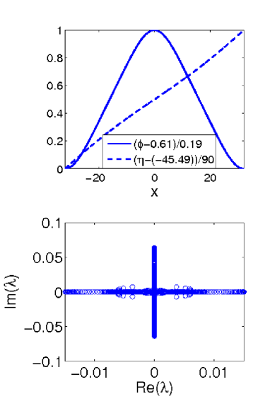
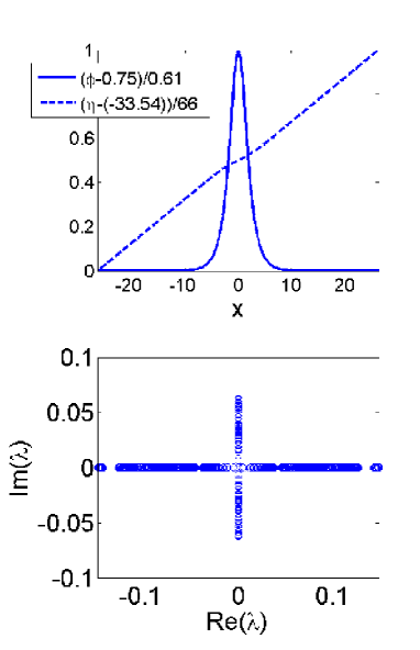
Figure 7: (Color Online) The top panels depict solution and phase and the bottom panels show the linear spectra. The left-hand solution is the elliptic solution given in Eq. (66) with $(a,b,c,m,g,A,B,D,F,G)=(0.5077,-0.9501,0.5,0.5,0.4145,0.1,0.7126,0,1,0.1155)$, while the right-hand solution is for the hyperbolic limit with $(a,b,c,m,g,A,B,D,F,G)=(1,-2,1,1,0.375,0.6124,0.75,0,1,0.7071)$.

4 Conclusions

To conclude, a large array of exact analytical solutions to various field theories were found leading directly to various exact solutions of cubic-quintic NLS and their stability and dynamics were studied numerically. The majority of these are oscillatory solutions which are unstable, however, some are found to be linearly stable, such as some elliptic solutions from the dark-soliton family solution II for appropriate parameter regimes. Also many hyperbolic dark-solitons were found to be stable and quite robust over a range of parameter values. The hyperbolic bright soliton solutions were found to be unstable to collapse when the cubic term is defocusing or nonexistent and the quintic term is focusing, while they were found to be always stable when the cubic term is focusing, for both focusing and defocusing quintic term (at least within the parametric regions examined herein). Some periodic solutions with defocusing and focusing cubic and quintic nonlinear terms, respectively, also displayed collapse phenomenon, while ones with a focusing cubic term did not.

Appendix A Solutions of $\phi^{2}$-$\phi^{3}$-$\phi^{4}$ and hence Quadratic-Cubic NLS Model

Let us consider solutions of field Eq. (12). As explained above, once these solutions are obtained, then the solution of the quadratic-cubic equation are immediately obtained from here by using Eqs. (1), (2) and (11). We list below eight distinct periodic solutions to the field Eq. (12). In each case, we also mention the values of the parameters $a,b,c$, in particular, if they are positive or negative. However, instead of Eq. (12) we use slightly different form given by

$$\phi_{xx}+2a\phi+3b\phi^{2}+4c\phi^{3}=0\,.$$ (100)

This is done so that one can easily pick up the solutions recently obtained by us in a related paper on coupled $\phi^{2}$-$\phi^{3}$-$\phi^{4}$ field theory [9].

Solution I

It is easily shown [9] that

$$\phi=F+A{\rm sn}(Bx+x_{0},m)\,,$$ (101)

is an exact solution to the field Eq. (100) provided

$$(1+m)B^{2}=-a\,,~{}~{}2(1+m)cA^{2}=ma\,,~{}~{}b=-4cF\,,~{}~{}b^{2}=4ac\,.$$ (102)

Thus this solution is valid provided $a<0,c<0$ while $b$ could be positive or negative.

In the limit $m=1$ the periodic solution (101) goes over to the dark soliton solution

$$\phi=F+A\tanh(Bx+x_{0})\,,$$ (103)

provided

$$2B^{2}=-a\,,~{}~{}4cA^{2}=a\,,~{}~{}b=-4cF\,,~{}~{}b^{2}=4ac\,.$$ (104)

Thus the dark soliton solution exists to field Eq. (100) provided $a<0,c<0$ while $b$ could be positive or negative.

Solution II

It is easily shown [9] that

$$\phi=F+A{\rm cn}(Bx+x_{0},m)\,,$$ (105)

is an exact solution to the field Eq. (100) provided

$$(2m-1)B^{2}=a\,,~{}~{}2cA^{2}=mB^{2}\,,~{}~{}b^{2}=4ac\,,b=-4cF\,.$$ (106)

Thus this solution is valid provided $a>0,c>0$ while $b$ could be positive or negative. Note also that this solution exists only if $m>1/2$.

In the limit $m=1$ the periodic solution (105) goes over to the bright soliton solution

$$\phi=F+A{\rm sech}(Bx+x_{0})\,,$$ (107)

provided

$$B^{2}=a\,,~{}~{}2cA^{2}=B^{2}\,,~{}~{}b^{2}=4ac\,,~{}~{}b=-4cF\,.$$ (108)

Thus the bright soliton solution exists to field Eq. (100) provided $a>0,c>0$ while $b$ could be either positive or negative.

Solution III

It is easily shown [9] that

$$\phi=F+A{\rm dn}(Bx+x_{0},m)\,,$$ (109)

is an exact solution to the field Eq. (100) provided

$$(2m-1)B^{2}=a\,,~{}~{}2cA^{2}=B^{2}\,,~{}~{}b^{2}=4ac\,,~{}~{}b=-4cF\,.$$ (110)

Thus this solution is valid provided $a>0,c>0$ while b could be either positive or negative. Note also that unlike solution II, this solution is valid for any $m(0\leq m\leq 1$).

In the limit $m=1$ the periodic solution (109) goes over to the bright soliton solution (107) and hence satisfy constraints given by Eq. (108).

Solution IV

It is easily shown [9] that

$$\phi=F+\frac{A{\rm sn}(Dx+x_{0},m)}{1+B{\rm dn}(Dx+x_{0},m)}\,,$$ (111)

is an exact solution to the field Eq. (100) provided

$$B=1\,,~{}~{}(2-m)D^{2}=-2a\,,~{}~{}4(2-m)cA^{2}=m^{2}a\,,~{}~{}b^{2}=4ac\,,~{}~{}b=-4cF\,.$$ (112)

Thus this solution is valid provided $a<0,c<0$ while $b$ could be either positive or negative.

In the limit $m=1$ the periodic solution (111) goes over to the dark soliton solution

$$\phi=F+\frac{A\tanh(Dx+x_{0})}{1+B{\rm sech}(Dx+x_{0})}\,,$$ (113)

provided

$$B=1\,,~{}~{}D^{2}=-2a\,,~{}~{}4cA^{2}=a\,,~{}~{}b^{2}=4ac\,,~{}~{}b=-4cF\,.$$ (114)

Thus the dark soliton solution exists to field Eq. (100) provided $a<0,c<0$ while $b$ could have either sign.

Solution V

It is easily shown [9] that

$$\phi=F+\frac{A{\rm cn}(Dx+x_{0},m)}{\sqrt{1-m}+B{\rm dn}(Dx+x_{0},m)}\,,$$ (115)

is an exact solution to the field Eq. (100) provided the parameters satisfy the same constraints as given by Eq. (112). Thus this solution is valid provided $a<0,c<0$ while $b$ could have either sign.

In the limit $m=1$ the periodic solution (115) goes over to a constant, i.e.

$$\phi=F+A\,,$$ (116)

where $F,A$ are as given by Eq. (114).

Solution IV

It is easily shown [9] that

$$\phi=F+\frac{A\tanh(Dx+x_{0})}{1+B\tanh(Dx+x_{0})}\,,$$ (117)

is an exact solution to the field Eq. (100) provided

$$~{}~{}2D^{2}=-a\,,~{}~{}A=F(1-B)\,,~{}~{}b^{2}=4ac\,,~{}~{}Fb=-(1+B)a\,.$$ (118)

Thus this solution is valid provided $a<0,c<0$ while $b$ could be either positive or negative.

Solution VII

It is easily shown [9] that

$$\phi=\frac{A{\rm sech}(Dx+x_{0})}{1+B{\rm sech}(Dx+x_{0})}\,,$$ (119)

is an exact solution to the field Eq. (100) provided

$$A=\frac{-2a}{\sqrt{b^{2}-4ac}}\,,~{}~{}D^{2}=-2a\,,~{}~{}B=\frac{b}{\sqrt{b^{2}-4ac}}\,.$$ (120)

Thus this solution is valid provided $a<0$ while $b,c$ could have either sign. In particular, if $c>0$ then $b$ can have either sign while if $c<0$ then $b>0$. This solution can also be rewritten as

$$\phi=\frac{-2a}{b+\sqrt{b^{2}-4ac}\cosh[\sqrt{2a}(x+x_{0})]}\,.$$ (121)

Solution VIII

It is easily shown [9] that

$$\phi=F+\frac{A{\rm sech}(Dx+x_{0})}{1+B{\rm sech}(Dx+x_{0})}\,,$$ (122)

is also an exact solution to the field Eq. (100) provided

$$A=-\frac{4a+3bF}{\sqrt{b^{2}+2bcF}}\,,~{}~{}D^{2}=3bF+4a\,,~{}~{}B=-\frac{b+4cF}{\sqrt{b^{2}+2bcF}}\,.$$ (123)

Thus this solution is valid provided $b>0,c<0$ while $a>(<$ or $=)0$ depending on if $m<(>$ or $=)1/5$.

Solution IX

It is easily shown that

$$\phi=\frac{Ax^{2}+B}{Dx^{2}+E}\,,$$ (124)

is an exact solution to the field Eq. (100) provided

$$AE=-3BD\,,~{}~{}\frac{A}{B}=-\frac{4a}{3}\,,~{}~{}9b^{2}=32ac\,,~{}~{}\frac{A}{D}=-\frac{4a}{3b}\,.$$ (125)

Thus this solution is only valid if $a>0,c>0$ while $b$ could be either positive or negative.

Appendix B Solutions of $\phi^{2}$-$\phi^{4}$ and hence Standard (Cubic) NLS Model

Finally, for completeness, we consider solutions of field Eq. (12). in case $b=0$. As explained above, once these solutions are obtained, then the solution of the standard (cubic) NLS equation are immediately obtained from here by using Eqs. (1), (2) and (11). We list below three distinct periodic solutions to the field Eq. (12) with $b=0$. In each case, we also mention the values of the parameters $a$ and $c$, in particular, if they are positive or negative. However, instead of Eq. (12) (with $b=0$) we use slightly different form given by

$$\phi_{xx}+2a\phi+4c\phi^{3}=0\,.$$ (126)

This is done so that one can easily pick up the solutions recently obtained by us in a related paper on coupled $\phi^{2}-\phi^{4}$ field theory [10].

Solution I

It is easily shown [10] that

$$\phi=A{\rm sn}(Bx+x_{0},m)\,,$$ (127)

is an exact solution to the field Eq. (126) provided

$$(1+m)B^{2}=2a\,,~{}~{}(1+m)cA^{2}=-ma\,.$$ (128)

Thus this solution is valid provided $a>0,c<0$.

In the limit $m=1$ the periodic solution (127) goes over to the dark soliton solution

$$\phi=A\tanh(Bx+x_{0})\,,$$ (129)

provided

$$B^{2}=a\,,~{}~{}2cA^{2}=-a\,.$$ (130)

Thus the dark soliton solution exists to field Eq. (126) provided $a>0,c<0$.

Solution II

It is easily shown [10] that

$$\phi=A{\rm cn}(Bx+x_{0},m)\,,$$ (131)

is an exact solution to the field Eq. (126) provided

$$(2m-1)B^{2}=-2a\,,~{}~{}(2m-1)cA^{2}=-ma\,.$$ (132)

Thus this solution is valid provided $c>0$ while $a<(>$ or $=)0$ depending on if $m>(<$ or $=)1/2$.

In the limit $m=1$ the periodic solution (131) goes over to the bright soliton solution

$$\phi=A{\rm sech}(Bx+x_{0})\,,$$ (133)

provided

$$B^{2}=-2a\,,~{}~{}cA^{2}=-a\,.$$ (134)

Thus the bright soliton solution exists to field Eq. (126) provided $a<0,c>0$.

Solution III

It is easily shown [10] that

$$\phi=A{\rm dn}(Bx+x_{0},m)\,,$$ (135)

is an exact solution to the field Eq. (126) provided

$$(2-m)B^{2}=-2a\,,~{}~{}(2-m)cA^{2}=-a\,.$$ (136)

Thus this solution is valid provided $a<0,c>0$.

In the limit $m=1$ the periodic solution (135) goes over to the bright soliton solution (133) and hence satisfy constraints given by Eq. (134).

References

• [1] See for example, C. Sulem and P.-L. Sulem, The Nonlinear Schrödinger Equation (Springer, New York, 1999).
• [2] C. De Angelis, IEEE J. Quantum Electron. 30, 818 (1994).
• [3] J. Atai and B.A. Malomed,Phys. Lett. A 284, 247 (2001).
• [4] F. Kh. Abdullaev, A. Gammal, L. Tomio and T. Frederico, Phys. Rev. A 63, 043604 (2001).
• [5] W. Zhang, E.M. Wright, H.Pu, and P. Meystre, Phys. Rev. A 68, 023605 (2003).
• [6] J. C. Bronski et al., Phys. Rev. Lett. 86, 1402 (2001); J. C. Bronski et al., Phys. Rev. E 63, 036612 (2001); J. C. Bronski et al., Phys. Rev. E 64, 056615 (2001).
• [7] Y. Zhu and J. Yang, Phys. Rev. E75, 036605 (2007).
• [8] A. Khare and A. Saxena, J. Math. Phys. 49 063301 (2008); arXiv: nlin/0609013.
• [9] A. Khare and A. Saxena, J. Math. Phys. 48, 043302 (2007); arXiv: nlin/0610032.
• [10] A. Khare and A. Saxena, J. Math. Phys. 47, 092902 (2006); arXiv: nlin/0608047.
• [11] M.G. Vakhitov and A.A. Kolokolov, Radiophys. Quantum Electron. 16, 783 (1973).
• [12] D. E. Pelinovsky, V. V. Afanasjev, and Y. S. Kivshar, Phys. Rev. E 53, 1940 (1996).
• [13] M.I. Weinstein, Commun. Pure App. Math 39, 51 (1986).
• [14] I. S. Gradshteyn and I. M. Ryzhyk, Tables of Integrals, Series and Products (Academic, San Diego, 1994).
• [15] P. F. Byrd and M. D. Friedman, Handbook of Elliptic Integrals for Engineers and Physicists (Springer-Verlag, Berlin, 1954).
• [16] L. D. Landau, J. Phys. (Moscow) 5, 71 (1941); L. D. Landau and E. M. Lifshitz, Fluid Mechanics (Pergamon Press, Oxford, 1959).
• [17] A. G. Sykes, M. J. Davis, and D. C. Roberts, Phys. Rev. Lett. 103, 085302 (2009).
• [18] B. Wu and Qian Niu, New J. Phys. 5, 104.1 (2003).