Tokunaga and Horton self-similarity
for level set trees of Markov chains

Abstract

The Horton and Tokunaga branching laws provide a convenient framework for studying self-similarity in random trees. The Horton self-similarity is a weaker property that addresses the principal branching in a tree; it is a counterpart of the power-law size distribution for elements of a branching system. The stronger Tokunaga self-similarity addresses so-called side branching. The Horton and Tokunaga self-similarity have been empirically established in numerous observed and modeled systems, and proven for two paradigmatic models: the critical Galton-Watson branching process with finite progeny and the finite-tree representation of a regular Brownian excursion. This study establishes the Tokunaga and Horton self-similarity for a tree representation of a finite symmetric homogeneous Markov chain. We also extend the concept of Horton and Tokunaga self-similarity to infinite trees and establish self-similarity for an infinite-tree representation of a regular Brownian motion. We conjecture that fractional Brownian motions are also Tokunaga and Horton self-similar, with self-similarity parameters depending on the Hurst exponent.

1 Introduction and motivation

Hierarchical branching organization is ubiquitous in nature. It is readily seen in river basins, drainage networks, bronchial passages, botanical trees, and snowflakes, to mention but a few (e.g., [1, 2, 3, 4]). Empirical evidence reveals a surprising similarity among various natural hierarchies — many of them are closely approximated by so-called self-similar trees (SSTs) [1, 2, 3, 5, 6, 7, 8, 9, 10, 11, 12, 13, 14, 15, 16]. An SST preserves its statistical structure, in a sense to be defined, under the operation of pruning, i.e., cutting the leaves; this is why the SSTs are sometimes referred to as fractal trees [2]. A two-parametric subclass of Tokunaga SSTs, introduced by Tokunaga [9] in a hydrological context, plays a special role in theory and applications, as it has been shown to emerge in unprecedented variety of modeled and natural phenomena. The Tokunaga SSTs with a broad range of parameters are seen in studies of river networks [1, 5, 8, 9, 10, 15, 17], vein structure of botanical leaves [2, 3], numerical analyses of diffusion limited aggregation [14, 18], two dimensional site percolation [19, 20, 21, 22], and nearest-neighbor clustering in Euclidean spaces [23]. The diversity of these processes and models hints at the existence of a universal (not problem-specific) underlying mechanism responsible for the Tokunaga self-similarity and prompts the question: What probability models may produce Tokunaga self-similar trees? An important answer to this question was given by Burd et al. [5] who studied Galton-Watson branching processes and have shown that, in this class, the Tokunaga self-similarity is a characteristic property of a critical binary branching, that is the discrete-time process that starts with a single progenitor and whose members equiprobably either split in two or die at every step. The critical binary Galton-Watson process is equivalent to the Shreve’s random river network model, for which the Tokunaga self-similarity has been known for long time [1, 5, 8, 15]. The Tokunaga self-similarity has also been rigorously established in a general hierarchical coagulation model of Gabrielov et al. [24] introduced in the framework of self-organized criticality, and in a random self-similar network model of Veitzer and Gupta [11] developed as an alternative to the Shreve’s random network model for river networks.

Prominently, the results of Burd et al. [5] reveal the Tokunaga self-similarity for any process represented by the finite Galton-Watson critical binary branching. In the context of this paper, the most important example is a regular Brownian motion, whose various connections to the Galton-Watson processes are well-known (see Pitman [25] for a modern review). For instance, the topological structure of the so-called $h$-excursions of a regular Brownian motion [26] and a Poisson sampling of a Brownian excursion [27] are equivalent to a finite critical binary Galton-Watson tree (Sect. 3 below explains the tree representation of time series), and hence these processes are Tokunaga self-similar.

This study further explores Tokunaga self-similarity by focusing on trees that describe the topological structure of the level sets of a time series or a real function, so-called level-set trees. Our set-up is closely related to the classical Harris correspondence between trees and finite random walks [28], and its later ramifications that include infinite trees with edge lengths [5, 17, 25, 29, 30, 31, 32, 33]. The main result of this paper is the Tokunaga and closely related Horton self-similarity for the level-set trees of finite symmetric homogeneous Markov chains (SHMCs) — see Sect. 5, Theorem 4. Notably, the Tokunaga and Horton self-similarity concepts have been defined so far only for finite trees (e.g., [5, 15, 34]). We suggest here a natural extension of Tokunaga and Horton self-similarity to infinite trees and establish self-similarity for an infinite-tree representation of a regular Brownian motion. The suggested approach is based on the forest of trees attached to the floor line as described by Pitman [25]. Finally, we discuss the strong distributional self-similarity that characterizes Markov chains with exponential jumps.

The paper is organized as follows. Section 2 introduces planar rooted trees, trees with edge lengths, Harris paths, and spaces of random trees with the Galton-Watson distribution. The trees on continuous functions are described in Sect. 3. Several types of self-similarity for trees — Horton, Tokunaga, and distributional self-similarity — are discussed in Sect. 4. The main results of the paper are summarized in Sect. 5. Section 6 addresses special properties of exponential Markov chains that, in particular, enjoy the strong distributional self-similarity. Proofs are collected in Sect. 7. Section 8 concludes.

2 Trees

We introduce here planar trees, the corresponding Harris paths, and the space of Galton-Watson trees following Burd et al. [5], Ossiander et al. [17] and Pitman [25].

2.1 Planar rooted trees

Recall that a graph $\mathcal{G}=(V,E)$ is a collection of vertices (nodes) $V=\{v_{i}\}$, $1\leq i\leq N_{V}$ and edges (links) $E=\{e_{k}\}$, $1\leq k\leq N_{E}$. In a simple graph each edge is defined as an unordered pair of distinct vertices: $\forall\,1\leq k\leq N_{E},\exists!\,1\leq i,j\leq N_{V},i\neq j$ such that $e_{k}=(v_{i},v_{j})$ and we say that the edge $k$ connects vertices $v_{i}$ and $v_{j}$. Furthermore, each pair of vertices in a simple graph may have at most one connecting edge.

A tree is a connected simple graph $T=(V,E)$ without cycles, which readily gives $N_{E}=N_{V}-1$. In a rooted tree, one node is designated as a root; this imposes a natural direction of edges as well as the parent-child relationship between the vertices. Specifically, we follow [5] to represent a labeled (planar) tree $T$ rooted at $\phi$ by a bijection between the set of vertices $V$ and set of finite integer-valued sequences $\langle i_{1},\dots,i_{n}\rangle\in T$ such that

• $\phi=\langle\emptyset\rangle$,

• if $\langle i_{1},\dots,i_{n}\rangle\in T$ then $\langle i_{1},\dots,i_{k}\rangle\in T\quad\forall\,1\leq k\leq n$, and

• if $\langle i_{1},\dots,i_{n}\rangle\in T$ then $\langle i_{1},\dots,i_{n-1},j\rangle\in T\quad\forall\,1\leq j\leq i_{n}$.

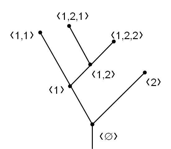
Figure 1: Representation of a tree via a set of finite sequences $\langle i_{1},\dots,i_{n}\rangle$.

This representation is illustrated in Fig. 1. If $v=\langle i_{1},\dots,i_{n}\rangle\in T$ then $u=\langle i_{1},\dots,i_{n-1}\rangle\in T$ is called the parent of $v$, and $v$ is a child of $u$. A leaf is a vertex with no children. The number of children of a vertex $u=\langle i_{1},\dots,i_{n}\rangle\in T$ equals to $c(u)=\max\{j\}$ over such $j$ that $\langle u,j\rangle\equiv\langle i_{1},\dots,i_{n},j\rangle\in T$. A binary labeled rooted tree is represented by a set of binary sequences with elements $i_{k}=1,2$, where 1,2 represent the left and right planar directions, respectively. Two trees are called distinct if they are represented by distinct sets of the vertex-sequences. We complete each tree $T$ by a special ghost edge $\epsilon$ attached to the root $\phi$, so each vertex in the tree has a single parental edge. A natural direction of edges is from a vertex $v$ to its parent $v_{p}$.

In these settings, the total number of distinct trees with $n$ leaves, according to the Cayley’s formula, is $n^{n-2}$. The total number of distinct binary trees with $n$ leaves is given by the $(n-1)$-th Catalan number [25]

$$C_{n-1}=\frac{1}{n}\left(\begin{array}[]{c}2n-2\\ n-1\end{array}\right).$$

2.2 Trees with edge-lengths and Harris path

A tree with edge-lengths $T=(V,E,W)$ assigns a positive lengths $w(e)$ to each edge $e$, $W=\{w(e)\}$; such trees are also called weighted trees (e.g., [5, 17]). The sum of all edge lengths is called the tree length; we write $\textsc{length}(T)=\sum_{e}\,w(e)$. We call the pair $(V,E)$ a combinatorial tree and write $(V,E)=\textsc{shape}(T)$, emphasizing that the lengths are disregarded in this representation.

If a tree is represented graphically in a plane, there is a unique continuous map

$$\sigma_{T}\,:\,[0,\,2\textsc{length}(T)]\to\,T$$

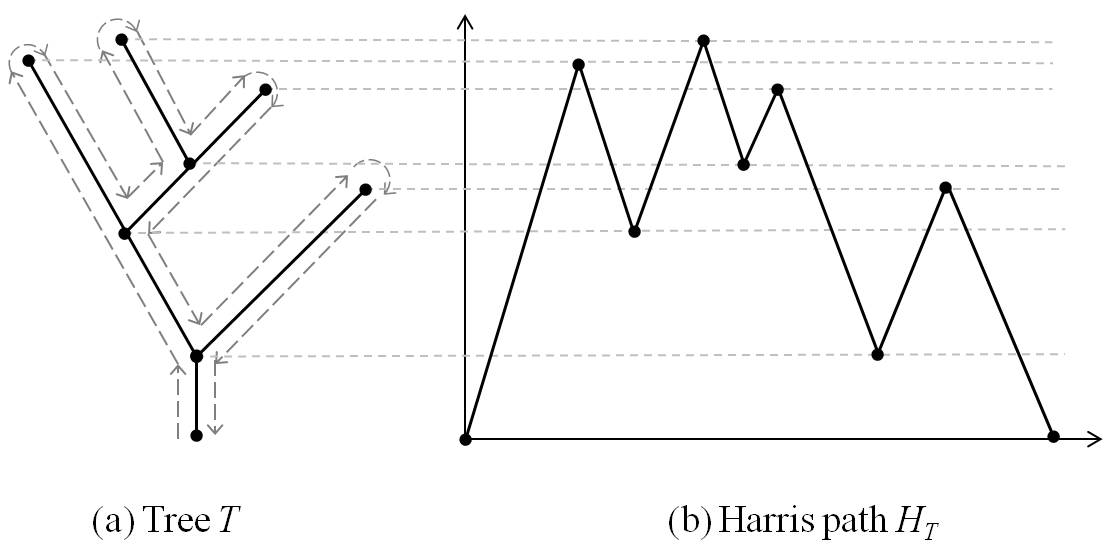
Figure 2: (a) Tree $T$ and its depth-first search illustrated by dashed arrows. (b) Harris path for the tree $T$ of panel (a).

that corresponds to the depth-first search of $T$, illustrated in Fig. 2(a). The depth-first search starts at the root of planar tree with edge-lengths and contours it, moving at a unit speed, from left to right so that each edge is traveled twice — its left side in a move away from the root, while its right side in a move towards the root. The Harris path for a tree $T$ is a continuous function $H_{T}(s)\,:\,[0,2\textsc{length}(T)]\to\mathbb{R}$ that equals to the distance from the root traveled along the tree $T$ in the depth-fist search. Accordingly, for a tree $T$ with $n$ leaves, the Harris path $H_{T}(s)$ is a continuous excursion — $H_{T}(0)=H_{T}(2\textsc{length}(T))=0$ and $H_{T}(s)>0$ for any $s\in\left(0,2\textsc{length}(T)\right)$ — that consists of $2n$ linear segments of alternating slopes $\pm 1$ [25], as illustrated in Fig. 2(b). The closely related Harris walk $H_{n}(k)$, $0\leq k\leq 2n$ for a tree with $n$ vertices is defined as a linearly interpolated discrete excursion with $2n$ steps that corresponds to the depth-first search that marks each vertex in a tree [28, 25]. Clearly, the Harris path and Harris walk, as functions $[0,2\textsc{length}(T)]\to\mathbb{R}$, have the same trajectory. A binary tree with $n$ leaves has $2n-1$ vertices; accordingly, its Harris path consists of $2n$ segments, and its Harris walk consists of $4n-2=2(2n-1)$ steps.

2.3 Galton-Watson trees

The space $\mathbb{T}$ of planar rooted trees with metric

$$d(\tau,\psi)=\frac{1}{1+\sup\{n:\tau|n=\psi|n\}},$$

where $\tau|n=\{\langle i_{1},\dots,i_{k}\rangle\in\tau:k\leq n\}$ form a Polish metric space, with the countable dense subset $\mathbb{T}_{0}$ of finite trees [17, 5]. An important, and most studied, class of distributions on $\mathbb{T}$ is the Galton-Watson distribution; it corresponds to the trees generated by the Galton-Watson process with a single progenitor and the branching distribution $\{p_{k}\}$. Formally, the distribution $GW_{\{p_{k}\}}$ assign the following probability to a closed ball $B\left(\tau,1/n\right)$, $\tau\in\mathbb{T}$, $n=1,2,\dots$:

$${\sf P}\left(B\left(\tau,\frac{1}{n}\right)\right)=\prod_{v\in\tau|(n-1)}p_{c(v)},$$

where $c(v)$ is the number of children of vertex $v$ [5, 17].

The classical work of Harris [28] notices that the Harris walk for a Galton-Watson tree with unit edge-lengths, $n$ vertices and geometric offspring distribution is an unsigned excursion of length $2n$ of a random walk with independent steps $\pm 1$. Hence, by the conditional Donsker’s theorem [25], a properly normalized Harris walk should weakly converge to a Brownian excursion. Aldous [29, 30, 31], LeGall [32, 33], and Ossiander et al. [17] have shown that the same limiting behavior is seen for a broader class of Galton-Watson trees, which may have non-trivial edge-lengths and non-geometric offspring distribution.

Theorem 1.

[17, Theorem 3.1] Let $T_{n}$ be a Galton-Watson tree with the total progeny $n$ and offspring distribution $L$ such that gcd$\{j:{\sf P}(L=j)>0\}=1$, ${\sf E}(L)=1$, and $0<{\sf Var}(L)=\sigma^{2}<\infty$, where gcd$\{\cdot\}$ denotes the greatest common divisor. Suppose that the i.i.d. lengths $W=\{w(e)\}$ are positive, independent of $T_{n}$, have mean 1 and variance $s^{2}$ and assume that $\lim_{x\to\infty}(x\,\log x)^{2}{\sf P}(|w(\phi)-1|>x)=0.$ Then the scaled Harris walk $H_{n}(k)$ converges in distribution to a standard Brownian excursion $B^{\rm ex}_{t}$:

$$\{H_{n}(2nt)/\sqrt{n},0\leq t\leq 1\}\overset{d}{\to}\{2\sigma^{-1}\,B^{\rm ex}_{t},0\leq t\leq 1\},\quad{\rm as~{}}n\to\infty.$$

This paper explores an “inverse” problem — it describes trees that correspond to a given finite or infinite Harris walk. We show, in particular, that the class of trees that correspond to the Harris walks that weakly converge to a Brownian excursion $B^{\rm ex}_{t}$ is much broader than the space of Galton-Watson trees.

3 Trees on continuous functions

Let $X_{t}\equiv X(t)\in C\left([L,R]\right)$ be a continuous function on a finite interval $[L,R]$, $L,R<\infty$. This section defines the tree associated with $X_{t}$. We start with a simple situation when $X_{t}$ has a finite number of local extrema and continue with general case.

3.1 Tamed functions: Level set trees

Suppose that the function $X_{t}\in C\left([L,R]\right)$ has a finite number of local extrema. The level set $\mathcal{L}_{\alpha}\left(X_{t}\right)$ is defined as the pre-image of the function values above $\alpha$:

$$\mathcal{L}_{\alpha}\left(X_{t}\right)=\{t\,:\,X_{t}\geq\alpha\}.$$

The level set $\mathcal{L}_{\alpha}$ for each $\alpha$ is a union of non-overlapping intervals; we write $|\mathcal{L}_{\alpha}|$ for their number. Notice that (i) $|\mathcal{L}_{\alpha}|=|\mathcal{L}_{\beta}|$ as soon as the interval $[\alpha,\,\beta]$ does not contain a value of local minima of $X_{t}$, (ii) $|\mathcal{L}_{\alpha}|\geq|\mathcal{L}_{\beta}|$ for any $\alpha>\beta$, and (iii) $0\leq|\mathcal{L}_{\alpha}|\leq n$, where $n$ is the number of the local maxima of $X_{t}$.

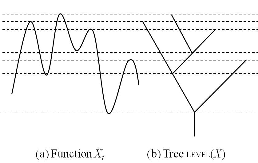
Figure 3: Function $X_{t}$ (panel a) with a finite number of local extrema and its level-set tree $\textsc{level}(X)$ (panel b).

The level set tree $\textsc{level}(X_{t})$ describes the topology of the level sets $\mathcal{L}_{\alpha}$ as a function of threshold $\alpha$, as illustrated in Fig. 3. Namely, there are bijections between (i) the leaves of $\textsc{level}(X_{t})$ and the local maxima of $X_{t}$, (ii) the internal (parental) vertices of $\textsc{level}(X_{t})$ and the local minima of $X_{t}$ (excluding possible local minima at the boundary points), and (iii) the edges of $\textsc{level}(X_{t})$ and the first positive excursions of $X(t)-X(t_{i})$ to right and left of each local minima $t_{i}$. The leftmost and rightmost edges $\langle 1,1,\dots,1\rangle$ and $\langle 2,2,\dots,2\rangle$ may correspond to meanders, that is to a positive segments of $X(t)-X(t_{i})$, rather than to excursions. It is readily seen that any function $X_{t}$ with distinct values of the local minima corresponds to a binary tree $\textsc{level}(X_{t})$. In this case, the bijection (iii) can be separated into the bijections between (iii a) the edges $\langle\dots,1\rangle$ of $\textsc{level}(X_{t})$ and the first positive excursions of $X(t)-X(t_{i})$ to the left of each local minima $t_{i}$, and (iii b) the edges $\langle\dots,2\rangle$ of $\textsc{level}(X_{t})$ and the first positive excursions of $X(t)-X(t_{i})$ to the right of each local minima $t_{i}$. The edge $e=(v,u)$ that connects the vertices $v$ and $u$ is assigned the length $w(e)$ equal to the absolute difference between the values of the respective local extrema of $X_{t}$ — according to the bijections (i), (ii) above.

To complete the above construction, a special care should be taken of the edge $\epsilon$ attached to the tree root. Specifically, let $t_{i}$, $i=1,\dots,n$, be the set of internal local minima of $X_{t}$, defined as the set of points such that for any $i$ there exists such an open interval $(a_{i},b_{i})\ni t_{i}$ that $X(t_{i})\leq X(s)$ for any $s\in(t_{i},b_{i})$, $X(t_{i})<X(b_{i})$, and $X(t_{i})<X(s)$ for any $s\in(a_{i},t_{i})$. The last definition treats only the leftmost point of any constant-level through as a local minima. The root of the tree $\textsc{level}(X_{t})$ corresponds to the lowest internal minimum. If the global minimum $M$ of $X_{t}$ is reached at one of the boundary points, say at $X(L)$, the root of $\textsc{level}(X_{t})$ has the parental edge $\epsilon$ with the length $w(\epsilon)=\min_{i}\left(X(t_{i})\right)-X(L)$. At the same time, if the global minimum $M$ of $X_{t}$, is reached at one of the internal local minima, that is if $M=\min_{i}\left(X(t_{i})\right)<\min\left(X(L),X(R)\right)$, then $|\mathcal{L}_{\alpha}|=0$ for any $\alpha<M$ and $|\mathcal{L}_{\alpha}|>1$ for any $\alpha>M$. In other words, the root of $\textsc{level}(X_{t})$ does not have the parental edge. In this case, we add the ghost parental edge $\epsilon$ with edge length $w(\epsilon)=1$. We write $\textsc{level}(X_{t},w(\epsilon))$ to explicitly indicate the length of the ghost edge that might be added to the level-set tree and save notation $w(\epsilon)$ for the value defined above uniquely for each function $X_{t}$.

By construction, the level set trees are invariant with respect to monotone transformations of time and values of $X_{t}$:

Proposition 1.

Let $F(\cdot)$ and $G(\cdot)$ be monotone functions such that $Y_{t}=F\left(X_{G(t)}\right)$ is a continuous function on $G\left([L,R]\right).$ Then the function $Y_{t}$ has the same combinatorial level set tree as the original function $X_{t}$, that is

$$\textsc{shape}\left(\textsc{level}(X_{t},1)\right)=\textsc{shape}\left(\textsc{level}(Y_{t},1)\right).$$

The tree with edge lengths $\textsc{level}(X_{t},1)$ is completely specified by the set of the local extrema of $X_{t}$ and its boundary values, and is independent of the detailed structure of the intervals of monotonicity. To formalize this observation, we write ${\mathcal{E}}_{X}(s)$ for the linear extreme function obtained from $X_{t}$ by (i) linearly interpolating its consecutive local extrema and the two boundary values, and (ii) changing time within each monotonicity interval as to have only constant slopes $\pm 1$. The function ${\mathcal{E}}_{X}(s)$ hence is a piece-wise linear function with slopes $\pm 1$. The length of the domain of this function equals the total variation of $X_{t}$. We shift this domain to start at $s_{0}=w(\epsilon)+X(L)-\min_{i}\left(X(t_{i})\right)$, where $t_{i}$ are the points of internal local minima as defined above.

Proposition 2.

The level set tree of a function $X_{t}$ coincides with that of the linear extreme function ${\mathcal{E}}_{X}$: $\textsc{level}(X_{t},1)=\textsc{level}\left({\mathcal{E}}_{X},1\right).$

The particular domain specification of ${\mathcal{E}}_{X}(z)$ is explained by the following statement.

Proposition 3.

Let $H_{T}(s)$, $s\in[0,2\textsc{length}(T)]$ be the Harris path of the level set tree $T=\textsc{level}(X_{t},1)$, then $H_{T}(z)={\mathcal{E}}_{X}(z)$ on the domain $D$ of ${\mathcal{E}}_{X}$. The domains of $H_{T}(z)$ and ${\mathcal{E}}_{X}(z)$ coincide, i.e. $D=[0,2\textsc{length}(T)]$, if and only if $X_{t}$ is a positive excursion, and $D\subset[0,2\textsc{length}(T)]$ otherwise.

It is known that each piece-wise linear positive excursion (Harris path) that consists of $2n$ segments with slopes $\pm 1$ uniquely specifies a tree $T$ with no vertices of degree 2 (e.g., [25]). Recall that a Harris path corresponds to the depth-first search that visits each edge in a tree twice; hence the Harris path $H_{T}$ over-specifies the corresponding tree $T$. Similarly, the function ${\mathcal{E}}_{X}(s)$ uniquely specifies (and, probably, over-specifies) the tree $\textsc{level}(X_{t},1)$ with no vertices of degree 2. If $X_{t}$ has distinct values of the local minima, then ${\mathcal{E}}_{X}(s)$ uniquely specifies the binary tree $\textsc{level}(X_{t},1)$.

Our definition of the level-set tree cannot be directly applied to a continuous function with infinite number of local extrema, say to a trajectory of a Brownian motion. This motivates the general set-up reviewed in the next section [25, 32].

3.2 General case

Let $X_{t}\equiv X(t)\in C\left([L,R]\right)$ and $\underline{X}[a,b]:=\inf_{t\in[a,b]}X(t)$, for any $a,b\in\,[L,R]$. We define a pseudo-metric on $[L,R]$ as

$$d_{X}(a,b):=\left(X(a)-\underline{X}[a,b]\right)+\left(X(b)-\underline{X}[a,b]\right),\quad a,b\in\,[L,R].$$ (1)

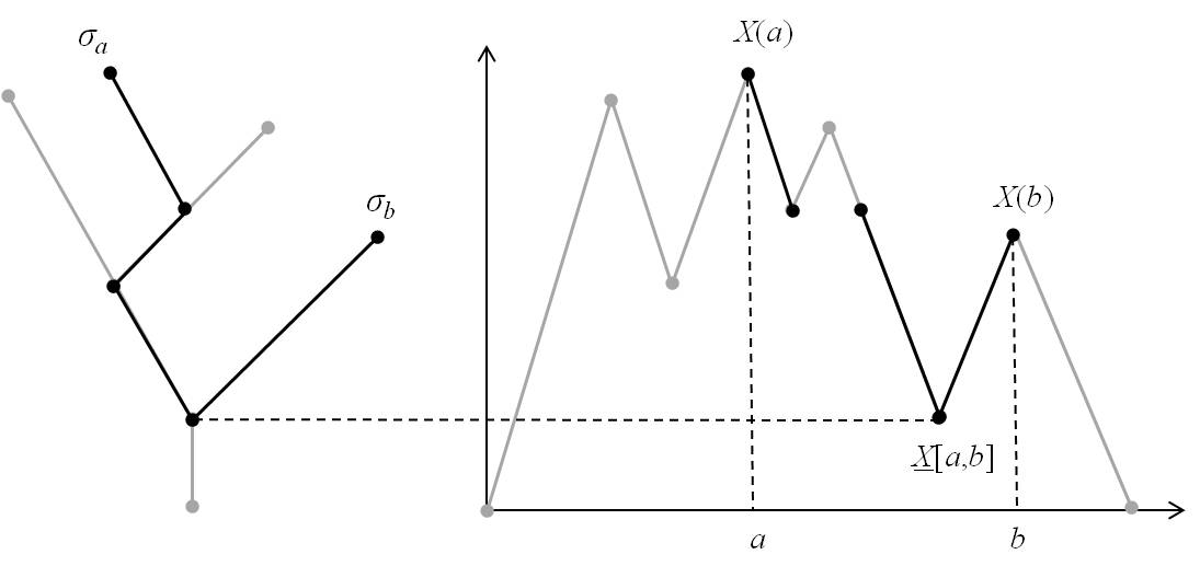
Figure 4: Illustration of the pseudo-distance $d_{X}(a,b)$ used to define the tree $\textsc{tree}(X)$ for a continuous function $X_{t}$. This example refers to a Harris path $X_{t}$ with the finite number of extrema, so one can construct a level set tree for $X_{t}$. Here, the local maxima $X(a)$ and $X(b)$ correspond to the leaves $\sigma_{a}$ and $\sigma_{b}$ in the tree shown on the left. The distance between these points is measured along the shortest path from $\sigma_{a}$ to $\sigma_{b}$ along the tree (marked by heavy lines), or equivalently, by Eq. (1).

It is easily verified that if $X_{t}$ is the Harris path for a finite tree $T$ and $\sigma_{T}$ is the corresponding depth-first search, then $d_{X}(a,b)$ equals the distance along the tree $T$ between the points $\sigma_{T}(a)$ and $\sigma_{T}(b)$ (see Fig. 4). We write $a\sim_{X}b$ if $d_{X}(a,b)=0$. Accordingly, we define tree $\textsc{tree}(X)$ for the function $X_{t}$ as the metric space $\left([L,R]/\sim_{X},d_{X}\right)$ [25].

Remark. The definition of the level set tree can be readily applied to a real-valued Morse function $f:\mathbb{M}\to\mathbb{R}$ on a smooth manifold $\mathbb{M}$. This is convenient for studying functions in higher-dimensional domains; see, for instance, Arnold [36] and Edelsbrunner et al. [37]. The Harris-path and metric-space definitions are not readily applicable to multidimensional domains.

4 Self-similar trees

This section describes the three basic forms of the tree self-similarity: (i) Horton laws, (ii) Self-similarity of side-branching, and (iii) Tokunaga self-similarity. They are based on the Horton-Strahler and Tokunaga schemes for ordering vertices in a rooted binary tree. The presented approach was introduced by Horton [6] for ordering hierarchically organized river tributaries; the methods was later refined by Strahler [7] and further expanded by Tokunaga [9] to include so-called side-branching.

4.1 Horton-Strahler ordering

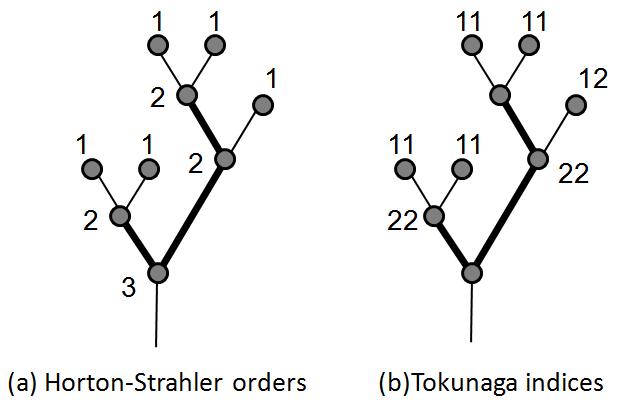
Figure 5: Example of (a) Horton-Strahler ordering, and of (b) Tokunaga indexing. Two order-2 branches are depicted by heavy lines in both panels. The Horton-Strahler orders refer, interchangeably, to the tree nodes or to their parent links. The Tokunaga indices refer to entire branches, and not to individual links.

The Horton-Strahler (HS) ordering of the vertices of a finite rooted labeled binary tree is performed in a hierarchical fashion, from leaves to the root [2, 5, 6, 7]: (i) each leaf has order $r({\rm leaf})=1$; (ii) when both children, $c_{1},c_{2}$, of a parent vertex $p$ have the same order $r$, the vertex $p$ is assigned order $r(p)=r+1$; (iii) when two children of vertex $p$ have different orders, the vertex $p$ is assigned the higher order of the two. Figure 5(a) illustrates this definition. Formally,

$$r(p)=\left\{\begin{array}[]{ll}r(c_{1})+1&{\rm if~{}}r(c_{1})=r(c_{2}),\\ \max\left(r(c_{1}),r(c_{2})\right)&{\rm if~{}}r(c_{1})\neq r(c_{2}).\end{array}\right.$$ (2)

A branch is defined as a union of connected vertices with the same order. The branch vertex nearest to the root is called the initial vertex, the vertex farthest from the root is called the terminal vertex. The order $\Omega(T)$ of a finite tree $T$ is the order $r(\phi)$ of its root, or, equivalently, the maximal order of its branches (or nodes). The magnitude $m_{i}$ of a branch $i$ is the number of the leaves descendant from its initial vertex. Let $N_{r}$ denote the total number of branches of order $r$ and $M_{r}$ the average magnitude of branches of order $r$ in a finite tree $T$.

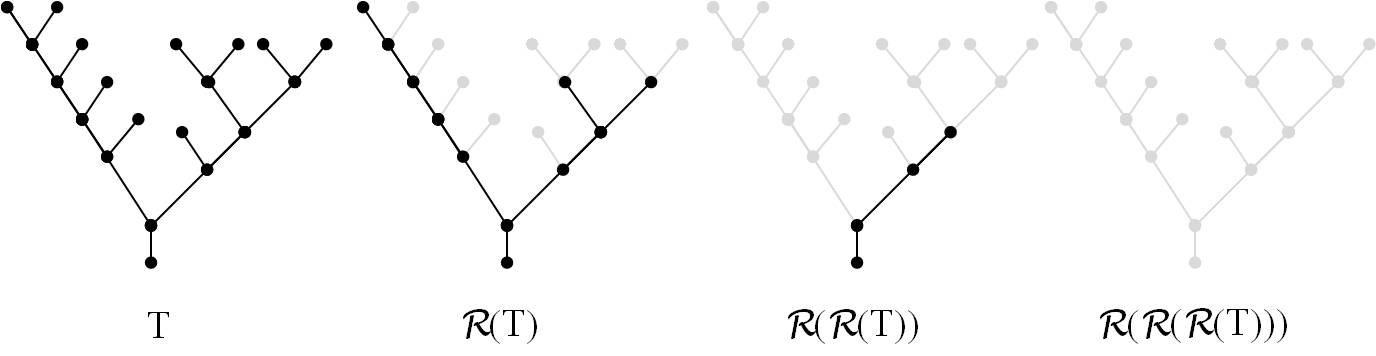
Figure 6: Example of consecutive application of the pruning operation ${\mathcal{R}}(\cdot)$ to the tree $T$. In this example the tree has order $\Omega=3$ so ${\mathcal{R}}^{(3)}(T)=\phi$. For visual convenience the pruned branches are shown in all panels by a light color. Notice that pruning may produce chains of single-child nodes.

An equivalent, and intuitively more appealing, definition of the Horton-Strahler orders is done via the operation of pruning [5, 15]. The pruning of an empty tree results in an empty tree, ${\mathcal{R}}(\phi)=\phi$. The pruning ${\mathcal{R}}(T)$ of a non-empty tree $T$, not necessarily binary, cuts the leaves and possible chains of degree-2 vertices connected to the leaves. A vertex of degree 2 (or a single-child vertex) $v$ is defined by the conditions $\langle v,1\rangle\in T$, $\langle v,2\rangle{\notin}T$. Each chain of degree-2 vertices connected to a leaf is uniquely identified by a vertex $v$ such that $\langle v,u\rangle\in T$ implies $u=\langle 1,\dots,1\rangle$. The pruning operation is illustrated in Fig. 6.

The first application of pruning to a binary tree $T$ simply cuts the leaves, possibly producing some single-child vertices. Some of those vertices are connected to the leaves via other single-child vertices and thus will be cut at the next pruning, while the other occur deeper within the pruned tree and will wait for their turn to be removed. It is readily seen that repetitive application of pruning to any tree will result in the empty tree $\phi$. The minimal $\Omega$ such that ${\mathcal{R}}^{(\Omega)}(T)=\phi$ is called the order of the tree. A vertex $v$ of tree $T$ has the order $r$ if it has been removed at the $r$-th application of pruning: $v\in{\mathcal{R}}^{(k)}(T)\,\forall 1\leq k<r$, $v\notin{\mathcal{R}}^{(r)}(T)$. We say that a binary tree $T$ is complete if any of the following equivalent statements hold: (i) each branch of $T$ consists of a single vertex; (ii) orders of siblings (vertices with the common parent) are equal; (iii) the parent vertex’s rank is a unit higher than that of each of its children. There exists only one complete binary tree on $n=2^{k}$ leaves for each $k=0,1,\dots$; all other trees are called incomplete.

4.2 Tokunaga indexing

The Tokunaga indexing [2, 9, 15] extends upon the Horton-Strahler orders; it is illustrated in Fig. 5b. This indexing focuses on incomplete trees by cataloging side-branching, which is the merging between branches of different order. Let $\tau^{k}_{ij}$, $1\leq k\leq N_{j}$, $1\leq i<j\leq\Omega$ denotes the number of branches of order $i$ that join the non-terminal vertices of the $k$-th branch of order $j$. Then $N_{ij}=\sum_{k}\,\tau^{k}_{ij}$, $j>i$ is the total number of such branches in a tree $T$. The Tokunaga index $T_{ij}$ is the average number of branches of order $i<j$ per branch of order $j$ in a finite tree of order $\Omega\geq j$:

$$T_{ij}=\frac{N_{ij}}{N_{j}}.$$ (3)

In a probabilistic set-up, one considers a space of finite binary trees with some probability measure. Then, $N_{i}$, $\tau_{ij}^{k}$, $N_{ij}$, and $T_{ij}$ become random variables. We notice that if, for a given $\{ij\}$, the side-branch counts $\tau_{ij}^{k}$ are independent identically distributed random variables, $\tau_{ij}^{k}\stackrel{{\scriptstyle d}}{{=}}\tau_{ij}$, then, by the law of large numbers,

$$T_{ij}\stackrel{{\scriptstyle\rm a.s}}{{\longrightarrow}}{\sf E}\left(\tau_{ij}\right)\quad{\rm as~{}}N_{j}\stackrel{{\scriptstyle\rm a.s}}{{\longrightarrow}}\infty,$$

where the almost sure convergence $X_{r}\stackrel{{\scriptstyle\rm a.s.}}{{\longrightarrow}}\mu$ is understood as ${\sf P}\left(\displaystyle\lim_{r\to\infty}X_{r}=\mu\right)=1$.

For consistency, we denote the total number of order-$i$ branches that merge with other order-$i$ branches by $N_{ii}$ and notice that in a binary tree $N_{ii}=2\,N_{i+1}$. This allows us to formally introduce the additional Tokunaga indices: $T_{ii}=N_{ii}/N_{i+1}\equiv 2.$ The set $\{T_{ij}\}$, $1\leq i\leq\Omega-1,1\leq j\leq\Omega$, $i\leq j$ of Tokunaga indices provides a complete statistical description of the branching structure of a finite tree of order $\Omega$.

Next, we define several types of tree self-similarity based on the Horton-Strahler and Tokunaga indexing schemes.

4.3 Horton laws

The Horton laws, widely observed in hydrological and biological networks [3, 6, 11, 12], state, in their ultimate form,

$$\frac{N_{r}}{N_{r+1}}=R_{B},\quad\frac{M_{r+1}}{M_{r}}=R_{M},\quad R_{B},R_{M}>0,\quad r\geq 1,$$

where $N_{r}$, $M_{r}$ is, respectively, the total number and average mass of branches of order $r$ in a finite tree of order $\Omega$. McConnell and Gupta [34] emphasized the approximate, asymptotic nature of the above empirical statements. In the present set-up, it will be natural to formulate the Horton laws as the almost sure convergence of the ratios of the branch statistics as the tree order increases:

$$\frac{N_{r}}{N_{r+1}} \stackrel{{\scriptstyle\rm a.s.}}{{\longrightarrow}} R_{B}>0,\quad{\rm for~{}}r\geq 1,{~{}\rm as~{}}\Omega\to\infty,$$ (4)

$$\frac{M_{r+1}}{M_{r}} \stackrel{{\scriptstyle\rm a.s.}}{{\longrightarrow}} R_{M}>0,\quad{\rm as~{}}r,\Omega\to\infty.$$ (5)

Notice that the convergence in (4) is seen for the small-order branches, while the convergence in (5) — for large-order branches. We call (4),(5) the weak Horton laws. We also consider strong Horton laws that assume an almost sure exponential dependence of the branch characteristics on $r$ in a tree of finite order $\Omega$ and magnitude $N$:

$$N_{r} \stackrel{{\scriptstyle\rm a.s.}}{{\sim}} N_{0}\,N\,R_{B}^{-r},\quad{\rm for~{}}r\geq 1,{~{}\rm as~{}}\Omega\to\infty,$$ (6)

$$M_{r} \stackrel{{\scriptstyle\rm a.s.}}{{\sim}} M_{0}\,R_{M}^{r},\quad{\rm as~{}}r,\Omega\to\infty$$ (7)

for some positive constants $N_{0},M_{0},R_{B}$ and $R_{M}$ and with $x_{r}\stackrel{{\scriptstyle\rm a.s.}}{{\sim}}y_{r}$ staying for

$${\sf P}\left(\displaystyle\lim_{r\to\infty}x_{r}/y_{r}=1\right)=1.$$

Clearly, the strong Horton laws imply the weak Horton laws. The inverse in general is not true; this can be illustrated by a sequence $M_{r}=R_{M}^{r}\,r^{C}$, for any $C>0$, for which the weak Horton law (5) holds, while the strong law (7) fails. We notice also that $\Omega\to\infty$ implies $N\to\infty$, but not vice versa; an example is given by a comb — a tree of order $\Omega=2$ with an arbitrary number of side branches with Tokunaga index $\{12\}$. This is why the limits above are taken with respect to $\Omega$, not $N$.

The strong Horton laws imply, in particular, that

$$N_{r}\stackrel{{\scriptstyle\rm a.s.}}{{\sim}}const\,M_{r}^{-\alpha},\quad\alpha=\frac{\log R_{B}}{\log R_{M}}$$ (8)

for appropriately chosen $r\to\infty$ and $\Omega\to\infty$, for instance $r=\sqrt{\Omega}$. The relationship (8) is the simplest indication of self-similarity, as it connects the number $N_{r}$ and the size $M_{r}$ of branches via a power law. However, a more restrictive property is conventionally required to call a tree self-similar; it is discussed in the next section.

4.4 Tokunaga self-similarity

In a deterministic setting, we call a tree $T$ of order $\Omega$ a self-similar tree (SST) if its side-branching structure (i) is the same for all branches of a given order:

$$\tau_{ij}^{k}=:\tau_{ij},\quad 1\leq k\leq N_{j},~{}1\leq i<j\leq\Omega,$$

and (ii) is invariant with respect to the branch order:

$$\tau_{i(i+k)}\equiv T_{i(i+k)}=:T_{k}\quad{\rm for~{}}2\leq i+k\leq\Omega.$$ (9)

A Tokunaga self-similar tree (TSST) obeys an additional constraint first considered by Tokunaga [9]:

$$T_{k+1}/T_{k}=c\quad\Leftrightarrow\quad T_{k}=a\,c^{k-1}\quad a,c>0,~{}1\leq k\leq\Omega-1.$$ (10)

In a random setting, we say that a tree $T$ of order $\Omega$ is self-similar if ${\sf E}\left(\tau_{i(i+k)}^{j}\right)=:T_{k}$ for $1\leq j\leq N_{i+k}$, $2\leq i+k\leq\Omega$; and it is Tokunaga self-similar if, furthermore, the condition (10) holds.

In a deterministic setting, for a tree satisfying the weak Horton and Tokunaga laws, one has [9, 15]:

$$R_{B}=\frac{2+c+a+\sqrt{(2+c+a)^{2}-8c}}{2}.$$ (11)

Peckham [15] has noticed that in a Tokunaga tree of order $\Omega$ one has $N_{r}=M_{\Omega-r+1}$, which implies that the Horton laws for masses $M_{r}$ follow from the Horton laws for the counts $N_{r}$ and $R_{M}=R_{B}$. McConnell and Gupta [34] have shown that the weak Horton laws with $R_{B}=R_{M}$ hold in a self-similar Tokunaga tree. Zaliapin [35] has shown, moreover, that strong Horton laws hold in a Tokunaga tree and, at the same time, even weak Horton laws may not hold in a general, non-Tokunaga, self-similar tree.

The Tokunaga self-similarity describes a two-parametric class of trees, specified by the Tokunaga parameters $(a,c)$. Our goal is to demonstrate that the Tokunaga class is not only structurally simple but is also sufficiently wide. This study establishes the Tokunaga self-similarity for the level-set trees of symmetric homogeneous Markov chains, and, as a direct consequence, for the trees of their scaling limits including a regular Brownian motion.

4.5 Stochastic self-similarity

Burd et al. [5] define stochastic self-similarity for a random tree $\tau\in\left(\mathbb{T}_{0},P\right)$ as the distributional invariance with respect to the pruning ${\mathcal{R}}(\tau)$:

$$P\left(\cdot|\tau\neq\phi\right)\circ{\mathcal{R}}^{-1}=P(\cdot)$$

and prove the following result that explains the importance of Tokunaga self-similarity within the class of Galton-Watson trees as well as the special role of the Galton-Watson critical binary trees.

Theorem 2.

[5, Theorems 1.1, 1.2, 3.17] Let $\tau\in\left(\mathbb{T}_{0},GW_{\{p_{k}\}}\right)$ with bounded offspring number. Then the following statements are equivalent:

• Tree $\tau$ is stochastically self-similar.

• ${\sf E}(\tau_{i(i+k)})=:T_{k}$, i.e., the expectation is a function of $k$ and $T_{k}$ is defined by this equation.

• Tree $\tau$ has the critical binary offspring distribution, $p_{0}=p_{2}=1/2$.

These authors show, furthermore, how the arbitrary binary Galton-Watson distribution is transformed under the operation of pruning.

Theorem 3.

[5, Proposition 2.1] Let $\tau$ be a finite tree with a binary Galton-Watson distribution, $p_{0}+p_{2}=1$, with $p_{2}\leq 1/2$. Let $\tau_{n+1}={\mathcal{R}}(\tau_{n})$, $n\geq 0$, $\tau_{0}=\tau$. Then $\tau_{n+1}$ has the binary Galton-Watson distribution $p_{0}^{(n+1)}+p_{2}^{(n+1)}=1$ with

$$p_{2}^{(n+1)}=\frac{\left[p_{2}^{(n)}\right]^{2}}{\left[p_{0}^{(n)}\right]^{2}+\left[p_{2}^{(n)}\right]^{2}}.$$

We demonstrate below that stochastic (or distributional) self-similarity, within the class of tree representations of homogeneous Markov chains, holds only for Markov chains with symmetric exponential increments.

5 Main results

Let $X_{k}$, $k\in\mathbb{Z}$ be a real valued Markov chain with homogeneous transition kernel $K(x,y)\equiv K(x-y)$, for any $x,y\in\mathbb{R}$. We call $X_{k}$ a homogeneous Markov chain (HMC). When working with trees, $X_{k}$ will also denote a function from $C(\mathbb{R})$ obtained by liner interpolation of the values of the original time series $X_{k}$; this create no ambiguities in the present context.

A HMC is called symmetric (SHMC) if its transition kernel satisfies $K(x)=K(-x)$ for any $x\in\mathbb{R}$. We call an HMC exponential (EHMC) if its kernel is a mixture of exponential jumps. Namely,

$$K(x)=p\,\phi_{\lambda_{u}}(x)+(1-p)\,\phi_{\lambda_{d}}(-x),\quad 0\leq p\leq 1,\lambda_{u},\lambda_{d}>0,$$

where $\phi_{\lambda}$ is the exponential density

$$\phi_{\lambda}(x)=\begin{cases}\lambda e^{-\lambda x},&x\geq 0,\\ 0,&x<0.\end{cases}$$ (12)

We will refer to an EHMC by its parameter triplet $\{p,\lambda_{u},\lambda_{d}\}$.

The concept of tree self-similarity is based on the notion of branch order and is tightly connected to the pruning operation (Sect. 4.1, Fig. 6). In terms of time series (or tamed real functions), pruning corresponds to coarsening the time series resolution by removing the local maxima. An iterative pruning corresponds to iterative transition to the local minima. We formulate this observation in the following proposition.

Proposition 4.

The transition from a time series $X_{k}$ to the time series $X^{(1)}_{k}$ of its local minima corresponds to the pruning of the level-set tree $\textsc{level}(X)$. Formally,

$$\textsc{level}\left(X^{(m)}\right)={\mathcal{R}}^{m}\left(\textsc{level}(X)\right),\forall m\geq 1,$$

where $X^{(m)}$ is obtained from $X$ by iteratively taking local minima $m$ times (i.e., local minima of local minima and so on.)

The next result establishes invariance of several classes of Markov chains with respect to the pruning operation.

Lemma 1.

(a) The local minima of a HMC form a HMC. (b) The local minima of a SHMC form a SHMC. (c) The local minima of an EHMC with parameters $\{p,\lambda_{u},\lambda_{d}\}$ form a EHMC with parameters $\{p^{*},\lambda_{u}^{*},\lambda_{d}^{*}\}$, where

$$p^{*}=\frac{p\,\lambda_{d}}{p\,\lambda_{d}+(1-p)\,\lambda_{u}},\quad\lambda^{*}_{d}=p\lambda_{d},~{}~{}\text{ and }~{}~{}\lambda^{*}_{u}=(1-p)\lambda_{u}.$$ (13)

Let $\{M_{t}\}\equiv\{M^{(1)}_{t}\}$, $t\in\mathcal{T}_{1}\subset\mathbb{R}$, be the set of local minima of $X_{t}$, not including the boundary minima; $\{M^{(2)}_{t}\}$, $t\in\mathcal{T}_{2}\subset\mathbb{R}$, be the set of local minima of local minima (local minima of second order), etc., with $\{M^{(j)}_{t}\}$, $t\in\mathcal{T}_{j}\subset\mathbb{R}$ being the local minima of order $j$. We call a segment between two consecutive points from $\mathcal{T}_{r}$, $r\geq 1$, a (complete) basin of order $r$. For each $r$, there might exist a single leftmost and a single rightmost segments of $X_{t}$ that do not belong to any basin or order $r$, with a possibility for them to merge if $X_{t}$ does not have basins of order $r$ at all. We call those segments incomplete basins of order $r$. There is a bijection between basins (complete and incomplete) of order $r$ in $X_{t}$ and branches of Horton-Strahler order $r$ in $\textsc{level}(X_{t})$. This explains the terms complete branch and incomplete branch of order $r$.

Theorem 4 (Horton and Tokunaga self-similarity).

The combinatorial level set tree $\textsc{shape}\left(\textsc{level}(X),1\right)$ of a finite SHMC $X_{k}$, $k=1,\dots,N$ satisfies the strong Horton laws for any $r\geq 1$, asymptotically in $N$:

$$N_{r}\overset{\rm a.s.}{\sim}N\,R_{\rm B}^{-r},\quad R_{\rm B}=4,\quad{\rm as~{}}N\to\infty.$$ (14)

Furthermore, $T=\textsc{shape}\left(\textsc{level}(X,1)\right)$ is a Tokunaga self-similar tree with parameters $(a,c)=(1,2)$. Specifically, for a finite tree $T$ of order $\Omega(N)$ the side-branch counts $\tau_{i(i+k)}^{j}$ with $2\leq i+k\leq\Omega$ for different complete branches $j$ of order $(i+k)$ are independent identically distributed random variables such that $\tau_{i(i+k)}^{j}\overset{d}{=:}\tau_{i(i+k)}$ and

$${\sf E}\left[\tau_{i(i+k)}\right]=:T_{k}=2^{k-1}.$$ (15)

Moreover, $\Omega\overset{a.s.}{\to}\infty$ as $N\to\infty$ and, for any $i,k\geq 1$, we have

$$T_{i(i+k)}\overset{\rm a.s.}{\longrightarrow}T_{k}=2^{k-1},\quad{\rm as~{}}N\to\infty,$$

where $T_{i(i+k)}$ can be computed over the entire $X_{k}$.

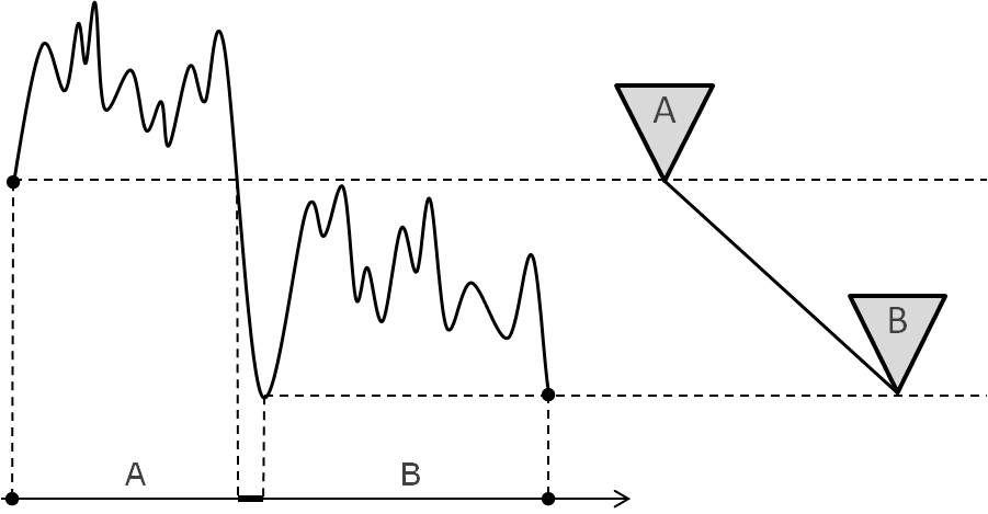
Figure 7: Illustration of tree construction for an infinite time series. The time series $X_{t}$ is divided here into two vertically shifted excursions, marked A and B in the time axis, and one fall, depicted by the heavy segment on the time axis. The descending ladder $L_{X}$ consists of two isolated points and one interval (heavy segment on the time axis). The excursions correspond to the two trees represented by marked triangles, the interval from the descending ladder corresponds to the line that connects the trees A and B.

Next we extend this result to the case of infinite time series and the weak limits of finite time series. For a linearly interpolated time series $X_{t}$, $t\geq 0$ (equivalently, for a continuous function with a countable number of separated local extrema) consider the descending ladder $L_{X}=\{t:X_{t}=\underline{X}[0,t]\}$, which in our settings is a set of isolated points and non-overlapping intervals (Fig. 7). The function $X_{t}$ is naturally divided into a series of vertically shifted positive excursions on the intervals not included in $L_{X}$ and monotone falls on the intervals from $L_{X}$. Any (in the a.s. sense) infinite SHMC can be decomposed into infinite number of such finite excursions and finite falls. We will index the excursions by index $i\geq 1$ from left to right. The extreme time series ${\mathcal{E}}\left(X_{k}^{i}\right)$ for each finite excursion $X_{t}^{i}$ is a Harris path for a finite tree $\textsc{level}\left(X_{t}^{i}\right)$. Hence, each such finite excursion completely specifies a single subtree of $\textsc{tree}\left(X_{t}\right)$. In particular, it completely specifies the HS orders for all vertices and Tokunaga indices for all branches except the one containing the root within $\textsc{level}\left(X_{t}^{i}\right)$. We also notice that each fall of $X_{t}$ on an interval from $L_{X}$ corresponds to an individual edge of $\textsc{tree}\left(X_{t}\right)$. Combining the above observations, we conclude that the tree $\textsc{tree}\left(X_{t}\right)$ can be represented as infinite number of subtrees $\textsc{level}(X_{t}^{i})$ connected by edges that correspond to the falls of $X_{t}$ on the descending ladder, see Fig. 7. Pitman calls this construction, applied to the standard Brownian motion rather than time series, a forest of trees attached to the floor line [25, Section 7.4]. Let $N_{r}^{n}$ and $N_{ij}^{n}$ denote, respectively, the number of branches of order $r$ and the number of side branches of Tokunaga index $\{ij\}$ in the first $n$ excursions of $X_{t}$ as described above. We introduce the cumulative quantities

$$\eta_{r}^{n}:=\frac{N_{r}^{n}}{N_{r+1}^{n}},\quad T_{ij}^{n}:=\frac{N_{ij}^{n}}{N_{j}^{n}}$$

and define, for the infinite time series $X_{t}$,

$$\eta_{r}(X_{t})=\lim_{n\to\infty}\eta_{r}^{n},\quad T_{ij}(X_{t})=\lim_{n\to\infty}T_{ij}^{n},$$ (16)

whenever the above limits exist in an appropriate probabilistic sense.

By Proposition 1, the level set tree of a finite excursion $X_{t}^{k}$ is not affected by monotonic transformations of time and value. This allows to expand the above definition (16) to the weak limits of time series via the the Donsker’s theorem. In particular, if $X_{t}$ is a SHMC whose increments have standard deviation $\sigma$, then the rescaled segments $X_{t}$ weakly converge to the regular Brownian motion $B_{t}$, $0\leq t\leq 1$. Namely,

$$X_{(nt)}/\sqrt{n}\overset{d}{\to}\sigma\,B_{t}$$

as $n\to\infty$ through the end point of the finite excursions that comprise $X_{t}$. This leads to the following result.

Corollary 1.

The combinatorial tree $\textsc{shape}\left(\textsc{tree}(B_{t})\right)$ of a regular Brownian motion $B_{t}$, $t\in[0,1]$ satisfies the Horton and Tokunaga self-similarity laws. Namely,

$$\eta_{r}(B_{t})=4~{}{\rm for~{}}r\geq 1\quad{\rm and}\quad T_{i(i+k)}(B_{t})=2^{k-1}~{}{\rm for~{}}i,k\geq 1,$$ (17)

where the limits (16) are understood in the almost sure sense.

We conclude this section with a conjecture motivated by the above result as well as extensive numeric simulations [23].

Conjecture 1.

The tree $\textsc{shape}\left(\textsc{tree}\left(B^{H}\right)\right)$ of a fractional Brownian motion $B^{H}_{t}$, $t\in[0,1]$ with the Hurst index $0<H<1$ is Tokunaga self-similar with $T_{i(i+k)}(B^{H})=T_{k}=c^{k-1}$, $c=2H+1$, $i,k\geq 1$. According to (11), this corresponds to the Horton self-similarity with

$$\eta_{r}(B^{H})=2+H+\sqrt{H^{2}+2},r\geq 1.$$ (18)

The sense of limits (16) is to be determined.

6 Exponential chains

This section focuses on exponential chains, which enjoy an important distributional self-similarity and whose level-set trees have the Galton-Watson distribution.

6.1 Distributional self-similarity

Consider a SHMC $X_{k}$, $k\in\mathbb{Z}$ with kernel

$$K(x)=\frac{f(x)+f(-x)}{2},$$

where $f(x)$ is a probability density function with support $\mathbb{R}^{+}$. The series of local minima of $X_{k}$ (or, equivalently, pruning $X_{k}^{(1)}$ of $X_{k}$) also forms a SHMC with transition kernel $K_{1}(x)$ (see Lemma 1(b)). It is natural to look for chains invariant with respect to the pruning:

$$X_{k}\overset{d}{=}c\,X_{k}^{(1)},c>0.$$ (19)

By Proposition 1, such invariance would guarantee the distributional Tokunaga self-similarity:

$$\tau_{i(i+k)}^{j}\overset{d}{=:}\tau_{i(i+k)}=T_{k},\quad 1\leq j\leq N_{i+k},1\leq i+k\leq\Omega,$$ (20)

where $T_{k}$ is a random number of side-branches of order $i$ that join an arbitrarily chosen branch of order $(i+k)$. Hence, we seek the conditions on $f(x)$ to ensure that $K_{1}(x)=c^{-1}K(x/c)$ for some constant $c>0$.

Proposition 5.

The local minima of a SHMC $X_{k}$ with kernel $K(x)$ form a SHMC with kernel

$$K_{1}(x)=\frac{K(x/c)}{c},\quad c>0$$

if and only if $c=2$ and

$$\Re\left[\widehat{f}(2s)\right]=\left|\frac{\widehat{f}(s)}{2-\widehat{f}(s)}\right|^{2},$$ (21)

where $\widehat{f}(s)$ is the characteristic function of $f(x)$ and $\Re[z]$ stays for the real part of $z\in\mathbb{C}$.

Observe that the set of densities $f(x)$ that satisfy (21) is not empty. A solution is given for example by the Laplace density with $\lambda>0$, e.g. for $f(x)=\phi_{\lambda}(x)$ with exponential density $\phi_{\lambda}(x)$ of (12), that is by an EHMC $\{1/2,\lambda,\lambda\}$.

6.2 Distributional self-similarity for symmetric exponential chains

Lemma 1(c) allows one to study the behavior of the EHMCs formed by local minima, minima of minima, and so on of an EHMC $X_{k}$ with parameters $\{p,\lambda_{u},\lambda_{d}\}$. Introducing the variables

$$A=\frac{1-p}{p},\quad\gamma=\frac{\lambda_{d}}{\lambda_{u}}$$ (22)

one readily obtains that their counterparts $\{A^{*},\gamma^{*}\}$ for the chain of local minima, given by (13), are expressed as

$$A^{*}=\frac{A}{\gamma},\quad\gamma^{*}=\frac{\gamma}{A}.$$ (23)

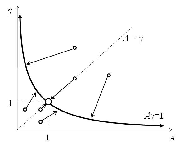
Figure 11: Characterization of EHMCs in the space $(A,\gamma)$ of (22) with iteration rules (23) that correspond to the transition to the EHMC of local maxima. Each EHMC corresponds to a point on the plane $(A,\gamma)$. The chain of local minima for any EHMC corresponds to a point on the hyperbola $A\,\gamma=1$. The point $(A=1,\gamma=1)$ is fixed. Any point from the lower branch ($A>1,\gamma<1$) moves along the hyperbola toward $(\infty,0)$. Any point from the upper branch ($A<1,\gamma>1$) moves along the hyperbola toward $(0,\infty)$. Arrows illustrate the point dynamics.

Notably, this means that the chain of local minima for any EHMC form an EHMC with $A\,\gamma=1$. The only fixed point in the space $(A,\gamma)$ with iteration rules (23) is the point $(A=1,\gamma=1)$, which corresponds to the distributionally self-similar EHMS discussed in Sect. 6.1. This point is an image (under the pruning operation) of the EHMCs with $A=\gamma$ or $p\,\lambda_{d}=(1-p)\,\lambda_{u}$. The last condition is equivalent to ${\sf E}(X_{k}-X_{k-1})=0$ for any $k>1$. The chain of local minima for any EHMC with $A>\gamma$ ($A<\gamma$) corresponds to a point on the upper (lower) part of the hyperbola $A\,\gamma=1$. Any point on this hyperbola, except the fixed point $(1,1)$, moves away from the fixed point toward $(0,\infty)$ or $(\infty,0)$. This is illustrated in Fig. 11. It follows that the Tokunaga and even weaker Horton self-similarity is only seen for a symmetric EHMC. The above discussion can be summarized in the following statement.

Theorem 5.

Let $X_{k}$ be an EHMC $\{p,\lambda_{u},\lambda_{d}\}$. Then $X_{k}$ satisfies the distributional self-similarity (19) if and only if $p=1/2$, $\lambda_{u}=\lambda_{d}$. Furthermore, the multiple pruning $X_{k}^{(m)}$, $m>1$ of $X_{k}$ satisfies the distributional self-similarity (19) if and only if the chain’s increments have zero mean, or, equivalently, if and only if $p\,\lambda_{d}=(1-p)\,\lambda_{u}$. In this case, the self-similarity is achieved after the first pruning, that is for the chain $X_{k}^{(1)}$ of local minima.

Corollary 2.

The regular Brownian motion with drift is not Tokunaga self-similar.

6.3 Connection to Galton-Watson trees

An important, and well known, fact is that the Galton-Watson distribution (see Sect. 2.3) is the characteristic property of trees that have Harris paths with alternating exponential steps. We formulate this result using the terminology of our paper.

Theorem 6.

[25, Lemma 7.3],[32, 26] Let $X_{k}$ be a discrete-time excursion with finite number of local minima. The level set tree $\textsc{shape}\left(\textsc{level}(X_{k},1)\right)$ is a binary Galton-Watson tree with $p_{0}+p_{2}=1$ if and only if the rises and falls of $X_{k}$, excluding the last fall, are distributed as independent exponential variables with parameters $(\mu+\lambda)$ and $(\mu-\lambda)$, respectively, for $0\leq\lambda<\mu$. In this case,

$$p_{0}=\frac{\mu+\lambda}{2\,\mu},\quad p_{2}=\frac{\mu-\lambda}{2\,\mu}.$$

We now use this result to relate sequential pruning of Galton-Watson trees (see Theorem 3) and pruning of EHMCs. Consider the first positive excursion $X_{k}$ of an EHMC with parameters $\{p^{(0)}=p=1-q,\lambda_{u},\lambda_{d}\}$. The geometric stability of the exponential distribution implies that the monotone rises and falls of $X_{k}$ are exponentially distributed with parameters $q\,\lambda_{u}$ and $p\,\lambda_{d}$, respectively. The Theorem 6 implies that $\textsc{shape}\left(\textsc{level}(X_{k})\right)$ is distributed as a binary Galton-Watson tree, $p_{0}+p_{2}=1$, with

$$p_{2}\equiv p_{2}^{(0)}=\frac{p\,\lambda_{d}}{q\,\lambda_{u}+p\,\lambda_{d}}.$$ (24)

The first pruning $X_{k}^{(1)}$ of $X_{k}$, according to (13), is the EHMC with parameters

$$\left\{p^{(1)}=\frac{p\,\lambda_{d}}{q\,\lambda_{u}+p\,\lambda_{d}},q\,\lambda_{u},p\,\lambda_{d}\right\}.$$

Its upward and downward monotone increments are exponentially distributed with parameters, respectively,

$$\frac{(q\,\lambda_{u})^{2}}{q\,\lambda_{u}+p\,\lambda_{d}}\quad{\rm and}\quad\frac{(p\,\lambda_{d})^{2}}{q\,\lambda_{u}+p\,\lambda_{d}}.$$

By Theorem 6, the level-set tree for an arbitrary positive excursion of $X_{k}^{(1)}$ is a binary Galton-Watson tree, $p_{0}^{(1)}+p_{2}^{(1)}=1$, with

$$p_{2}^{(1)}=\frac{(p\,\lambda_{d})^{2}}{(q\,\lambda_{u})^{2}+(p\,\lambda_{d})^{2}}.$$

Continuing this way, we find that $n$-th pruning $X_{k}^{(n)}$ of $X_{k}\equiv X_{k}^{(0)}$ is an EHMCs such that the level set tree of its arbitrary positive excursion have a binary Galton-Watson distribution, $p_{0}^{(n)}+p_{2}^{(n)}=1$, with

$$p_{2}^{(n)}=\frac{(p\,\lambda_{d})^{2^{n}}}{(q\,\lambda_{u})^{2^{n}}+(p\,\lambda_{d})^{2^{n}}}.$$

This can be rewritten in recursive form as

$$p_{2}^{(n)}=\frac{\left[p_{2}^{(n-1)}\right]^{2}}{\left[p_{0}^{(n-1)}\right]^{2}+\left[p_{2}^{(n-1)}\right]^{2}},\quad n\geq 1$$

with $p_{2}^{(0)}$ given by (24). Notably, this is the same recursive system as that discovered by Burd et al. [5, Proposition 2.1] (see Theorem 3 above) in their analysis of consecutive pruning for the Galton-Watson trees. Another noteworthy relation is given by

$$p^{(n)}=p_{2}^{(n-1)},\quad n\geq 1,\quad p^{(0)}=p,p_{2}^{(0)}=p_{2},$$

which connects the “horizontal” probability $p^{(n)}$ of an upward jump in a pruned time series $X_{k}^{(n)}$ with the “vertical” probability $p_{2}^{(n-1)}$ of branching in a Galton-Watson tree.

7 Terminology and proofs

7.1 Level-set trees: Definitions and terminology

This section introduces terminology for discussing the hierarchical structure of the local extrema of a finite time series $X_{k}$ and relating it to the level set tree $\textsc{level}(X)$. For consistency we repeat some terms introduced above to formulate Theorem 4.

Let $\{M_{t}\}\equiv\{M^{(1)}_{t}\}$, $t\in\mathcal{T}_{1}\subset\mathbb{R}$, be the set of local minima of $X_{t}$, not including possible boundary minima; $\{M^{(2)}_{t}\}$, $t\in\mathcal{T}_{2}\subset\mathbb{R}$, be the set of local minima of local minima (local minima of second order), etc., with $\{M^{(j)}_{t}\}$, $t\in\mathcal{T}_{j}\subset\mathbb{R}$ being the local minima of order $j$. Next, let $\{m_{s}\}\equiv\{m^{(1)}_{s}\}$, $s\in\mathcal{S}_{1}\subset\mathbb{R}$, be the set of local maxima of $X_{k}$, including possible boundary maxima, and $\{m^{(j+1)}_{s}\}$, $s\in\mathcal{S}_{j+1}\subset\mathbb{R}$ the set of local maxima of $\{M^{(j)}_{t}\}$ for all $j\geq 1$. We will call a segment between two consecutive points from $\mathcal{T}_{j}$ a (complete) basin of order $j$. Clearly, $\mathcal{T}_{1}\supset\mathcal{T}_{2}\supset\dots$ and each basin of order $r$ is comprised of a non-zero number of basins of arbitrary order $k<r$. For each $r$, there might exist a single leftmost and a single rightmost segments of $X_{t}$ that do not belong to any basin or order $r$, with a possibility for them to merge if $X_{t}$ does not have basins of order $r$ at all. We call those segments incomplete basins of order $r$.

By construction, each basin of order $j$ contains exactly one point from $\mathcal{S}_{j}$; e.g., there is a single local maximum from $\mathcal{S}_{1}$ between two consecutive local minima from $\mathcal{T}_{1}$, etc. There exists a bijection between basins (complete and incomplete) of order $r$ in $X_{t}$ and branches of Horton-Strahler order $r$ in $\textsc{level}(X_{t})$; this explains the terms complete branch and incomplete branch of order $r$. More specifically, there is a bijection between the terminal vertices of order-$r$ branches — i.e., vertices parental to two branches of order $(r-1)$ — and the local maxima from $\mathcal{S}_{j}$ within the respective basins.

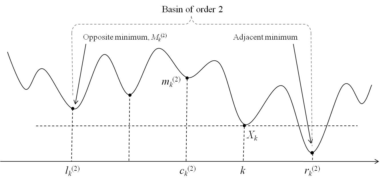
Figure 9: Basin of order 2: an illustration. The figure shows a basin of order 2 that consists of 5 local minima. The figure illustrates the taxonomy used in the paper; it shows the local maximum $m_{k}^{(2)}$ of the basin’s local minima, the opposite and adjacent minima of second order for a local minimum $X_{k}$, as well as the corresponding points $l^{(2)}_{k}$, $c^{(2)}_{k}$, and $r^{(2)}_{k}$.

Let us fix an arbitrary local minimum $X_{k}$ of order $r_{k}$; then $k\in\mathcal{T}_{j}$ for $1\leq j\leq r_{k}$ and $k\notin\mathcal{T}_{j}$ for $j>r_{k}$. For each $j>r_{k}$ there exists a unique basin of order $j$ that contains $k$; we denote the boundaries of this basin by $l_{k}^{(j)},r_{k}^{(j)}\in\mathcal{T}^{(j)}$, $l_{k}^{(j)}<r_{k}^{(j)}$. Denote by $c^{(j)}_{k}$ the unique point from $\mathcal{S}_{j}$ within the interval $\left(l_{k}^{(j)},r_{k}^{(j)}\right)$. Multiple points $X_{k}$ may correspond to the same triplet $\left(l_{k}^{(j)},c^{(j)}_{k},r_{k}^{(j)}\right)$, which will create no confusion. These definitions are illustrated in Fig. 9.

Consider now a point $k$ of local minimum such that $k\notin\cup_{j\geq 1}m^{(j)}_{s}$. If $l_{k}^{(j)}<k<c^{(j)}_{k}$ for a given $j>r_{k}$ then we call the point $l_{k}^{(j)}$ the local minimum of order $j$ adjacent to $k$ and the point $r_{k}^{(j)}$ the local minimum of order $j$ opposite to $k$. The analogous terminology is introduced in case $c_{k}^{(j)}<k<r^{(j)}_{k}$. By construction, $X_{k}$ is always greater than the value of its adjacent minimum of any order $j>r_{k}$. The value of the opposite minimum of order $j$ is denoted by $M^{(j)}_{k}$. We have, for each $k$,

$$M^{(1)}_{k}\geq M^{(2)}_{k}\geq M^{(3)}_{k}\geq\dots$$ (25)

We already noticed that the local maxima $m^{(1)}_{t}$ correspond to the tree leaves, that is to its branches of Horton order $r=1$. The set $m^{(j+1)}_{t}$ for each $j\geq 1$ corresponds to the vertices parental to two branches of the same HS order $j$; they are the terminal vertices of order-$(j+1)$ branches. All other local minima of $X_{k}$ correspond to vertices parental to two vertices of different SH order; we will refer to this as side-branching. Specifically, a local minimum $X_{k}$ of order $i$ forms a side-branch of order $\{ij\}$ if

$$M^{(j-1)}_{k}\geq X_{k}\geq M^{(j)}_{k},$$ (26)

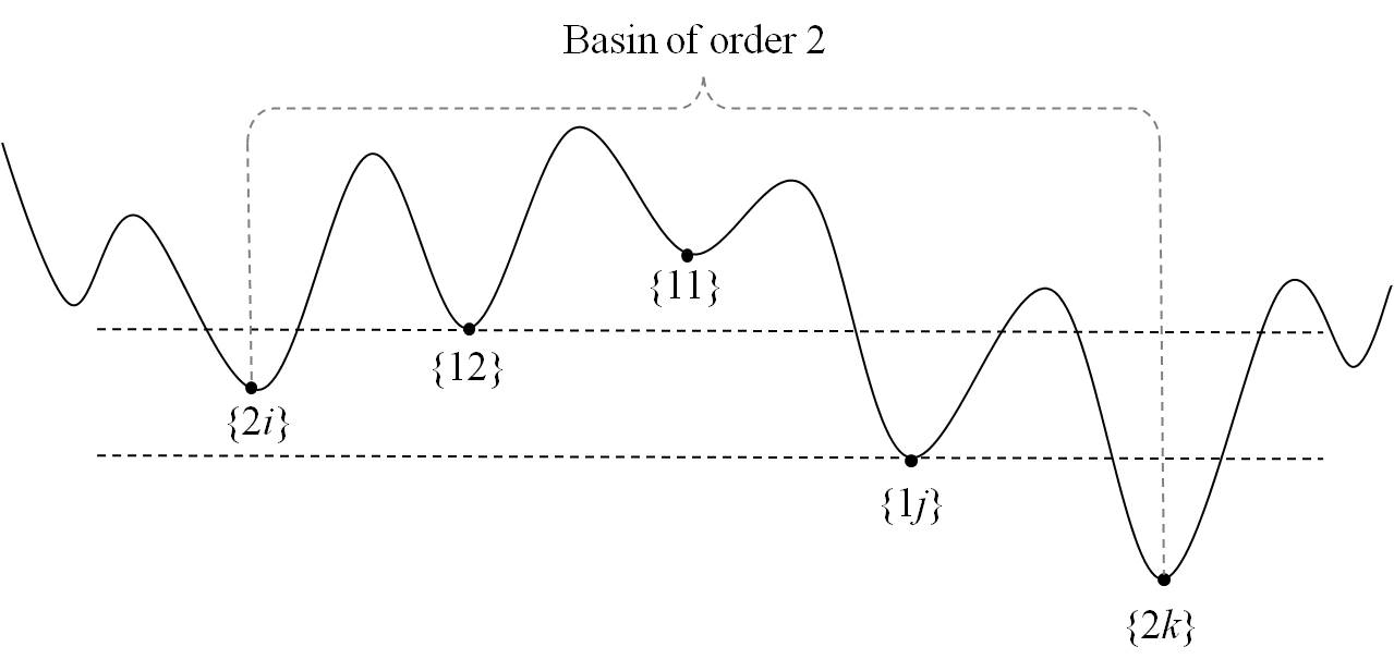
Figure 10: Tokunaga indexing: an illustration. The figure shows the Tokunaga indexing for the local minima of the second order basin shown in Fig. 9. The values of $i,j,k>2$ are determined by the large-scale structure of the function $X_{t}$.

where the first inequality disappears when $j=i+1$. Figure 10 illustrates this for a basin of second order. In general, each basin of order $r$ contains a uniquely specified positive excursion attached to its higher end. The local maxima of order $k<r$ from this excursion correspond to the side-branches with Tokunaga index $\{km\}$ with $m\leq r$. The local maxima of order $k<r$ within the basin but outside of this excursion correspond to the side-branches with Tokunaga index $\{km\}$ with $m>r$.

7.2 Proofs

Proof of Propositions 1,2,3 and 4: The statements readily follow from the definition of level set trees. ∎

Proof of Lemma 1:

(a) Follows from the independence of increments in $X_{k}$.

(b) Let $\{M_{j}\}$ be the sequence of local minima of $X_{k}$ and $d_{j}=M_{j+1}-M_{j}$. We have, for each $j$

$$d_{j}=\sum_{i=1}^{\xi_{+}}Y_{i}-\sum_{i=1}^{\xi_{-}}Z_{i},$$ (27)

where $\xi_{+}$ and $\xi_{-}$ are independent geometric random variables with parameter $1/2$:

$${\sf P}(\xi_{+}=k)={\sf P}(\xi_{-}=k)=2^{-k},\quad k=1,2,\dots;$$

$Y_{i}$, $Z_{i}$ are independent identically distributed (i.i.d.) random variables with density $f(x)$. Here the first sum corresponds to $\xi_{+}$ positive increments of $X_{k}$ between a local minimum $M_{j}$ and the subsequent local maximum $m_{j}$ and the second sum to $\xi_{-}$ negative increments between the local maximum $m_{j}$ and the subsequent local minimum $M_{j+1}$. It is readily seen that both the sums in (27) have the same distribution, and hence their difference has a symmetric distribution. We notice that the symmetric kernel for the sequence of local minima $\{M_{j}\}$ is necessarily different from $K(x)$.

(c) Consider an EHMC $X_{k}$ with parameters $\{p,\lambda_{u},\lambda_{d}\}$. By statement (a) of this lemma, the local minima of $X_{k}$ form a HMC with transition kernel $K_{1}(x)$. The latter is the probability distribution of the jumps $d_{j}$ given by (27) with $\xi_{+}$, $\xi_{-}$ being geometric random variables with parameters $p$ and $(1-p)$ respectively, $Y_{i}\overset{d}{=}\phi_{\lambda_{u}}$, and $Z_{i}\overset{d}{=}\phi_{\lambda_{d}}$. For the characteristic function of $K_{1}$ one readily has

$$\widehat{K_{1}}(s)=\frac{p(1-p)\lambda_{d}\lambda_{u}}{\left((1-p)\lambda_{u}-is\right)(p\lambda_{d}+is)}=p_{*}\cdot\widehat{\phi_{\lambda^{*}_{u}}}(s)+(1-p_{*})\cdot\widehat{\phi_{\lambda^{*}_{d}}}(-s)$$

with

$$p_{*}=\frac{p\,\lambda_{d}}{p\,\lambda_{d}+(1-p)\,\lambda_{u}},\quad\lambda^{*}_{d}=p\lambda_{d},~{}~{}\text{ and }~{}~{}\lambda^{*}_{u}=(1-p)\lambda_{u}.$$

Thus

$$K_{1}(x)=p_{*}\phi_{\lambda^{*}_{u}}(x)+(1-p_{*})\phi_{\lambda^{*}_{d}}(-x).$$

This means that the HMC of local minima also jumps according to a two-sided exponential law, only with different parameters $p_{*}$, $\lambda^{*}_{d}$ and $\lambda^{*}_{u}$. ∎

Proof of Theorem 4: Horton self-similarity

We notice that the number $N_{r}$ of order-$r$ branches in $\textsc{level}(X)$ equals the number $|{\mathcal{S}}_{r}|$ of local maxima $m^{(r)}_{s}$ of order $r$ (with the convention that the local maxima of order 0 are the values of $X_{k}$). The probability for a given point of $X_{k}$ to be a local maximum equals the probability that this point is higher than both its neighbors. The Markov property and symmetry of the chain imply that this probability is $1/4$. Hence the average number of local maxima is

$${\sf E}\left(|{\mathcal{S}}_{0}|\right)={\sf E}\left(N_{1}\right)=\sum_{i=2}^{N-1}{\sf P}(X_{i-1}<X_{i}>X_{i+1})=\frac{N-2}{4}\sim\frac{N}{4}.$$

Let $l_{i}$ denote the event ($X_{i}$ is a local maximum). By Markov property, the events $l_{i}$, $l_{j}$ are independent for $|i-j|\geq 2$; hence, the variance ${\sf V}(N_{1})\propto N$. This yields

$$\lim_{N\to\infty}{\sf E}\left(\frac{N_{1}}{N}\right)=1/4,\quad\lim_{N\to\infty}{\sf V}\left(\frac{N_{1}}{N}\right)=0.$$

One can combine the strong laws of large numbers for (i) the proportion of the upward increments of $X_{t}$ (that converges to 1/2) and (ii) the proportion of upward increments followed by a downward increment (that converges to 1/2) to obtain $N_{1}/N\overset{\rm a.s.}{\to}1/4$, and, in particular, $N_{1}\overset{\rm a.s.}{\to}\infty$ as $N\to\infty$.

We use now Lemma 1(b) to find, applying the same argument to the pruned time series, that $N_{r}/N_{r-1}\overset{\rm a.s.}{\to}1/4$ as $N\to\infty$ for any $r>1$. Finally,

$$\frac{N_{r}}{N}=\frac{N_{r}}{N_{r-1}}\frac{N_{r-1}}{N_{r-2}}\dots\frac{N_{1}}{N}\overset{\rm a.s.}{\longrightarrow}4^{-r},\quad N\to\infty,$$

which completes the proof of the strong Horton law (14). ∎

The proof of the Tokunaga self-similarity will require several auxiliary statements formulated below.

Lemma 2.

A basin of order $j$ contains on average $4^{j-k}$ basins of order $k$, for any $j>k\geq 1$.

Proof of Lemma 2: We show first that a basin of order $(j+1)$ contains on average 4 local minima of order $j\geq 1$. The number $\xi$ of points of $X_{k}$ within a first-order basin (i.e., between two consecutive local minima) is $\xi=1+\xi_{+}+\xi_{-}$, where $\xi_{+}$, $\xi_{-}$ are, respectively, the numbers of basin points (excluding the basin boundaries) to the left and right of its local maximum $m$; and the latter is counted separately in the expression above. The independence of increments of $X_{k}$ impies

$${\sf P}(\xi_{+}=k)={\sf P}(\xi_{-}=k)=2^{-k-1},k=0,1,\dots,$$

and hence

$${\sf E}[\xi]=1+{\sf E}[\xi_{+}]+{\sf E}[\xi_{-}]=1+1+1=3.$$ (28)

By Lemma 1(b), the same result holds for the average number of local minima of order $j$ within an order-$(j+1)$ basin, for any $j\geq 1$. Thus, the average number of order-$j$ basins within an order-$(j+1)$ basin is ${\sf E}[\xi]+1=4.$

The independence of increments of $X_{k}$ implies that the number of order-$(j-1)$ subbasins within an order-$j$ basin is independent of the numbers of order-$j$ basins within an order-$(j+1)$ basin. This leads to the Lemma’s statement. ∎

Lemma 3.

Let $a$ and $b$ be two points chosen at random and without replacement from the set $\{1,2,\dots,N\}$ and $\eta=(\eta_{1},\eta_{2},\eta_{3})$ denotes the random number of points within the following intervals respectively: (i) $\left[1,\,\min(a,b)\right)$, (ii) $\left(\min(a,b),\,\max(a,b)\right)$, and (iii) $\left(\max(a,b),\,N\right]$. Then the triplet $\eta$ has an exchangeable distribution.

Proof of Lemma 3: We notice that the triplet $\eta$ can be equivalently constructed by choosing three points $(a,b,c)$ at random from $(N+1)$ points on a circle and counting the number of points within each of the three resulting segments. This implies exchangeability.

∎

Lemma 4.

Let $Y_{i}\in\mathbb{R}$, $i=1,2,\dots$ be i.i.d. random variables, a pair $(n,m)\in\mathbb{N}^{2}$ has an exchangeable distribution independent of $Y_{i}$, and

$$X=\sum_{i=1}^{n}Y_{i}-\sum_{i=n+1}^{n+m}Y_{i}.$$ (29)

Then $X$ has a symmetric distribution.

Proof of Lemma 4: Let $\Delta=n-m$ and $F(X\,|\,\Delta)$ denote the conditional distribution of $X$ given $\Delta$. From the definition of $X$ it follows that

$$F(X\,|\,\Delta=k)=F(-X\,|\,\Delta=-k).$$

Exchangeability of $(n,m)$ implies symmetry of $\Delta$ and we thus obtain

$$F(X) = \sum_{k=-\infty}^{\infty}F(X\,|\,\Delta=k)\,{\sf P}(\Delta=k)$$

$$= \sum_{k=0}^{\infty}\left[F(X\,|\,\Delta=k)+F(X\,|\,\Delta=-k)\right]\,{\sf P}(\Delta=k)$$

$$= \sum_{k=0}^{\infty}\left[F(X\,|\,\Delta=k)+F(-X\,|\,\Delta=k)\right]\,{\sf P}(\Delta=k).$$

The sums of conditional distributions in brackets are symmetric, which completes the proof. ∎

Proof of Theorem 4: Tokunaga self-similarity

We will show that $\displaystyle\lim_{N\to\infty}T_{ij}=2^{j-i-1}$ for any pair $j>i$. By Lemma 1(b), $T_{ij}=T_{(i+k)\,(j+k)}$ and so it suffices to prove the statement for $i=1$, that is to show that $\displaystyle\lim_{N\to\infty}T_{1j}=2^{j-2}$ for any $j\geq 2$. This will be done by induction. Below we use the terminology introduced in Sect. 7.1.

Induction base, $j=2$. Consider a basin of order 2, formed by two consecutive points from $\mathcal{T}_{2}$ (local minima of second order). We denote here their positions by $L$ and $R$, $L<R$. This part of the proof will consider only local minima from this interval; they will be referred to as “points”.

The highest local minimum, or point $c=c_{k}^{(2)}\in\mathcal{S}_{2}$ forms a vertex parental to two branches of order 1 with Tokunaga indices $\{11\}$; in addition, a random number of local minima corresponds to internal vertices parental to side-branches with Tokunaga indices $\{1j\}$, $j>1$. The number $N^{(L,R)}_{12}$ of vertices of index $\{12\}$ within $(L,R)$ equals the number of side-branch points $X_{k}$ that are higher than their opposite minimum of second order:

$$N^{(L,R)}_{12}=\#\{L<k<R\,:\,X_{k}>M^{(2)}_{k}\}.$$

For each side-branch vertex $X_{k}$ we necessarily have $X_{k}<X_{c}$ since $X_{c}$ is maximal among the local minima. Recall that the local minima form a SHMC. Hence, for a randomly chosen side-branch $X_{k}$ we have

$$X_{c}-X_{k}=\sum_{i=1}^{\xi^{\prime}}Y_{i},$$

where $\xi^{\prime}$ is a geometric rv such that ${\sf P}(\xi^{\prime}=k)=2^{-k}$, and $Y_{i}>0$ are i.i.d. random variables that correspond to the jumps between the local minima. Clearly, the difference $X_{c}-M^{(2)}_{k}$ has the same distribution. The random variables $(X_{c}-M^{(2)}_{k})$ and $(X_{c}-X_{k})$ are independent and so ${\sf P}\left(X_{k}>M^{(2)}_{k}\right)=1/2$. The expected number of side-branches with index $\{12\}$ within the interval $(L,R)$ is

$${\sf E}\left[N^{(L,R)}_{12}\right]={\sf E}\left[\sum_{k=1}^{\xi-1}{\rm 1\rule{0.43057pt}{6.54443pt}\hskip 0.86108pt}_{(0,\infty)}\left(X_{k}-M^{(2)}_{k}\right)\right].$$ (30)

The summation above is taken over $(\xi-1)$ side-branch points within $(L,R)$; and the random variables $\xi$ was described in Lemma 2.

We show next that the random variables ${\rm 1\rule{0.43057pt}{6.54443pt}\hskip 0.86108pt}_{(0,\infty)}\left(X_{k}-M^{(2)}_{k}\right)$ are independent of $\xi$. Suppose that there exist $\xi=N$ points within $(L,R)$. A particular placement of $k$ and $c$ among these points is obtained by choosing two points at random and without replacement from $\{1,\dots,N\}$. By Lemma 3, the conditional distribution of the numbers of points between $k$ and $c$ and between $c$ and the local minimum opposite to $X_{k}$ have an exchangeable distribution. Lemma 4 implies that ${\sf P}\left(X_{k}>M^{(2)}_{k}\,|\,\xi=N\right)=1/2$. Thus,

$${\sf E}\left[N^{(L,R)}_{12}\right]={\sf E}[\xi-1]\,{\sf P}\left(X_{k}>M^{(2)}_{k}\right)=2\times 1/2=1.$$ (31)

The numbers $N_{12}^{(L,R)}$ are independent for different basins of order 2 by Markov property of $X_{t}$. The strong law of large numbers yields

$$T_{12}=\frac{N_{12}}{N_{2}}\overset{\rm a.s.}{\longrightarrow}1=2^{0}~{}{\rm as~{}}N\to\infty.$$

Induction step. Suppose that the statement is proven for $j\geq 2$, that is we know that for a randomly chosen local minima $X_{k}$

$${\sf P}\left(X_{k}>M^{(j)}_{k}\right)=2^{-(j-1)}$$

and $T_{1j}\overset{\rm a.s.}{\to}2^{j-2}$ as $N\to\infty$. We will prove it now for $(j+1)$. Consider a randomly chosen side-branch point $X_{k}$ of order $\{1i\}$, $i>j$. By (26), $X_{k}<M^{(m)}_{k}$ for $1\leq m\leq j$ and thus necessarily $X_{k}<c_{k}^{(i+1)}$, $1\leq i\leq j$, since $c_{k}^{(i+1)}$ is a local maximum of order-$i$ minima within the basin $(L,R)$ of order $(j+1)$ that contains $k$. Repeating the argument of the induction base we find that $X_{k}-M_{k}^{(i)}$ has a symmetric distribution for all $i\leq j+1$ and that the probability of $(X_{k}>M_{k}^{(i)})$ is independent of the number of local maxima of order $j$ within the basin $(L,R)$. This gives, for a randomly chosen $X_{k}$,

$${\sf P}\left(X_{k}>M^{(j+1)}_{k}\right) = {\sf P}\left(X_{k}>M^{(j+1)}_{k},X_{k}>M^{(j)}_{k}\right)$$

$$= {\sf P}\left(X_{k}>M^{(j+1)}_{k}\left|X_{k}>M^{(j)}\right.\right)\,{\sf P}\left(X_{k}>M^{(j)}_{k}\right)$$

$$= 2^{-1}\times 2^{-(j-1)}=2^{-j}.$$

By Lemma 2, the average number of order-2 basins within a basin of order $(j+1)$ is $4^{j-1}$. Each such basin contains on average 2 points that correspond to side branches with Tokunaga index $\{1\bullet\}$. Hence, the average total number of side-branches with index $\{1\bullet\}$ within a basin of order $(j+1)$ is $2\times 4^{j-1}=2^{2j-1}$. Applying the Wald’s lemma to the sum of indicators ${\rm 1\rule{0.43057pt}{6.54443pt}\hskip 0.86108pt}_{(0,\infty)}(X_{k}-M^{(j+1)}_{k})$ over the random number of local minima of order $j$ within the basin $(L,R)$, we find the average total number of side-branches of order $\{1(j+1)\}$:

$${\sf E}\left[N^{(L,R)}_{1(j+1)}\right]=2^{-j}\times 2^{2j-1}=2^{j-1}.$$

The strong law of large numbers yields

$$T_{1(j+1)}=\frac{N_{1(j+1)}}{N_{(j+1)}}\overset{\rm a.s.}{\longrightarrow}2^{j-1},~{}{\rm as~{}}N\to\infty.$$

∎

Proof of Proposition 5: Each transition step between the local minima of $X_{k}$ can be represented as $d_{j}$ of (27) where $\{Y_{i}\}$ and $\{Z_{i}\}$ are independent random variables with density $f(x)$, and $\xi_{+}$ and $\xi_{-}$ are two independent geometric random variables with parameter $1/2$. The Wald’s lemma readily implies that $c=2$. This gives for the characteristic functions

$$\widehat{K}_{1}(s)=2\,\widehat{K}(2s)=\Re\left[\widehat{f}(2s)\right].$$

On the other hand, taking the characteristic function of $d_{j}$ we obtain

$$\widehat{K}_{1}(s)=\left|\frac{\widehat{f}(s)}{2-\widehat{f}(s)}\right|^{2},$$

which completes the proof. ∎

Proof of Theorem 5: The Tokunaga and Horton self-similarity for a symmetric EHMC was proven in Theorem 4. Here we show the violation of the Horton self-similarity for an asymmetric EHMC.

Let $X^{(m)}_{k}$ denote the time series obtained by $m$-time repetitive pruning of time series $X_{k}$. Recall that there is one-to-one correspondence between the local maxima of $X^{(m)}$ and the branches of order $m$ in the level set tree $\textsc{level}(X)$ (see Sect. 7.1). Hence, the Horton self-similarity is equivalent to the invariance of the proportion of local maxima with respect to pruning. The proportion of local maxima in $X^{(m)}$ equals the probability $P^{(m)}_{\rm min}$ for a randomly chosen point to be a local maxima. The Markov property of $X^{(m)}$ — Lemma 1(c) — implies that $P^{(m)}_{\rm min}=p^{(m)}(1-p^{(m)})$, where $p^{(m)}$ is the probability for an upward jump in $X^{(m)}$.

For an asymmetric EHMC let $A^{(m)}$ be the $m$-th iteration of $A$, as in (22), (23). There, for $m\geq 1$, either $A^{(m)}<1$ in which case $A^{(m)}\to 0$ or $A^{(m)}>1$ in which case $A^{(m)}\to\infty$, all as $m\to\infty$ (see Sect. 6.2, Eq. (23) and Fig. 11). This corresponds to $p^{(m)}=1/(A^{(m)}+1)\to 1$ or $p^{(m)}\to 0$, respectively, and leads to $P^{(m)}_{\rm min}\to 0$. This prohibits the Horton, and hence Tokunaga, self-similarity. ∎

8 Discussion

This work establishes the Tokunaga and Horton self-similarity for the level-set tree of a finite symmetric homogeneous Markov process with discrete time and continuous state space (Sect. 5, Theorem 4). We also suggest a definition of self-similarity for an infinite tree, using the construction of a forest of subtrees attached to the floor line [25]; this allows us to establish the Tokunaga and Horton self-similarity for a regular Brownian motion (Sect. 5, Corollary 1). This particular extension to infinite trees seems natural for tree representation of time series, where concatenation of individual finite time series corresponds to the “horizontal” growth of the corresponding tree. Alternative definitions might be better suited though for other situations related, say, to the “vertical” growth of a tree from the leaves, like in a branching process.

A useful observation is the equivalence of smoothing the time series by removing its local maxima and pruning the corresponding level-set tree (Sect. 5, Proposition 4). It allows one to switch naturally between the tree and time-series domains in studying various self-similarity properties.

As discussed in the introduction, the Tokunaga self-similarity for various finite-tree representations of a Brownian motion follow from (i) the results of Burd et al. [5] on the Tokunaga self-similarity for the critical binary Galton-Watson process and (ii) equivalence of a particular tree representation to this process. We suggest here an alternative, direct approach to establishing Tokunaga self-similarity in Markov processes. Not only this approach does not refer to the Galton-Watson property, it extends the Tokunaga self-similarity to a much broader class of trees. Indeed, as shown by Le Gall [32] and Neveu and Pitman [26] (see Theorem 6), the tree representation of any non-exponential symmetric Markov chain is not Galton-Watson; it is still Tokunaga, however, by our Theorem 4.

Peckham and Gupta [16] have introduced the generalized Horton laws, which state the equality in distributions for the rescaled versions of suitable branch statistics $S_{r}$: $S_{r}\overset{d}{=}R_{S}^{r-k}\,S_{k}$, $R_{S}>0$. These authors established the existence of the generalized Horton laws in the Shreve’s random model, that is for the Galton-Watson trees. Accordingly, one would expect the generalized Horton laws to hold for the exponential symmetric Markov chains. Veitzer and Gupta [11] and Troutman [38] have studied the random self-similar network (RSN) model introduced in order to explain the variability of the limiting branching ratios in the empirical Horton laws. They have demonstrated that the extended Horton laws hold for various branch statistics, including the average magnitudes $M_{r}$, in this model. Furthermore, they established the weak Horton laws (4), (5) and Tokunaga self-similarity for the RSN model. Notably, the RSN model does not belong to the class of Galton-Watson trees, yet it demonstrates the Tokunaga self-similarity, similarly to the non-exponential symmetric Markov chains considered here.

Tree representation of stochastic processes [25, 26, 29, 30, 31, 32, 33] and real functions [36, 37] is an intriguing topic that attracts attention of mathematicians and natural scientists. A structurally simple yet flexible Tokunaga self-similarity, which extends beyond the classical Galton-Watson space, may provide a useful insight into the structure of existing data sets and models as well as suggest novel ways of modeling various natural phenomena. For instance, the level set tree representation have been used recently in analysis of the statistical properties of fragment coverage in genome sequencing experiments [39, 40, 41]. It seems that some of the methods and results obtained in this work might prove useful for the gene studies. In particular, it looks intriguing to test the self-similarity of the gene-related trees and interpret it in the biological context.

Notably, the results of this paper, as well as that of Burd et al. [5], refer only to a single point $(a,c)=(1,2)$ in the two-dimensional space of Tokunaga parameters. The empirical and numerical studies, however, report a broad range of these parameters, roughly $1<a<2$ and $1<c<4$. This motivates a search for more general Tokunaga models; a potential broad family is suggested by our Conjecture 1.

The construction of the level set tree is a particular case of the coagulation process; in the real function context it describes the hierarchical structure of the embedded excursions of increasing lengths and heights. Coagulation theory — a well-established field with broad range of practical applications to physics, biology, and social sciences [42, 43, 4] — is heavily based on the concepts of symmetry and exchangeability [25, 42]. We find it noteworthy that the only property used to establish the results in this paper is symmetry of a Markov chain. It seems worthwhile to explore the concept of Tokunaga self-similarity for a general coalescent process.

Acknowledgement. We are grateful to Ed Waymire and Don Turcotte for providing continuing inspiration to this study. We also thank Mickael Chekroun, Michael Ghil, Efi Foufoula-Georgiou, and Scott Peckham for their support and interest to this work. Comments of two anonymous reviewers helped us to significantly improve and expand an earlier version of this work. This study was supported by the NSF Awards DMS 0620838 and DMS 0934871.

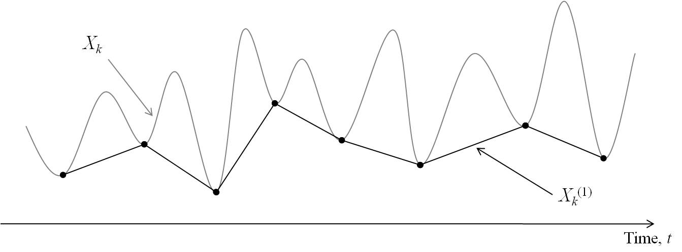
Figure 8: Time series $X_{k}$ (light line) and the series $X_{k}^{(1)}$ of linearly connected local minima (black line and dots).

References

- [1] R.L. Shreve, Statistical law of stream numbers, J. Geol., 74 (1966) 17–37.
- [2] W.I. Newman, D.L. Turcotte, A.M. Gabrielov, Fractal trees with side branching, Fractals. 5 (1997) 603–614.
- [3] D.L. Turcotte, J.D. Pelletier, and W.I. Newman, Networks with side branching in biology, J. Theor. Biol. 193 (1998) 577–592.
- [4] M.E.J. Newman, A.-L. Barabasi, and D.J. Watts, The Structure and Dynamics of Networks, Princeton University Press, 2006.
- [5] G.A. Burd, E.C. Waymire, R.D. Winn A self-similar invariance of critical binary Galton-Watson trees, Bernoulli. 6 (2000) 1–21.
- [6] R.E. Horton, Erosional development of streams and their drainage basins: Hydrophysical approach to quantitative morphology, Geol. Soc. Am. Bull. 56 (1945) 275–370.
- [7] A.N. Strahler, Quantitative analysis of watershed geomorphology, Trans. Am. Geophys. Un., 38 (1957) 913–920.
- [8] R.L. Shreve, Stream lengths and basin area in topologically random channel networks, J. Geol, 77, (1969) 397–414.
- [9] E. Tokunaga, Consideration on the composition of drainage networks and their evolution, Geographical Rep. Tokyo Metro. Univ., 13 (1978) 1–27.
- [10] D.G. Tarboton, R.L. Bras, I. Rodriguez-Iturbe, The fractal nature of river networks, Water Resources Res. 24 (1988) 1317 -1322.
- [11] S. Veitzer, V.K. Gupta (2000), Random self-similar river networks and derivations of generalized Horton laws in terms of statistical simple scaling, Water Resour. Res. 36 (2000) 1033- 1048.
- [12] P.S. Dodds, D.H. Rothman, Scaling, Universality, and Geomorphology, Ann. Rev. Earth and Planet. Sci., 28 (2000) 571–610. doi:10.1146/annurev.earth.28.1.571.
- [13] J.D. Pelletier, D.L. Turcotte, Shapes of river networks and leaves: Are they statistically similar? Phil. Trans. R. Soc. London B. 355 (2000) 307–311.
- [14] P. Ossadnik, Branch Order and Ramification Analysis of Large Diffusion Limited Aggregation Clusters, Phys. Rev. A. 45 (1992) 1058.
- [15] S.D. Peckham, New results for self-similar trees with applications to river networks, Water Resources Res. 31 (1995) 1023–1029.
- [16] S. Peckham, V. Gupta, A reformulation of Horton’s laws for large river networks in terms of statistical self-similarity, Water Resour. Res. 35 (1999) 2763–2777.
- [17] M. Ossiander, E. Waymire, Q. Zhang, Some width function asymptotics for weighted trees Ann. Appl. Prob., 7, 4 (1997) 972–995.
- [18] J.G. Masek, D.L. Turcotte, A Diffusion Limited Aggregation Model for the Evolution of Drainage Networks, Earth Planet. Sci. Let. 119 (1993) 379.
- [19] D.L. Turcotte, B.D. Malamud, G. Morein, W. I. Newman, An inverse cascade model for self-organized critical behavior, Physica, A. 268 (1999) 629 -643.
- [20] G. Yakovlev, W.I. Newman, D.L. Turcotte, A. Gabrielov An inverse cascade model for self-organized complexity and natural hazards, Geophys. J. Int. 163 (2005) 433–442.
- [21] I. Zaliapin, H. Wong, A. Gabrielov, Inverse cascade in percolation model: Hierarchical description of time-dependent scaling, Phys. Rev. E. 71 (2006) No. 066118.
- [22] I. Zaliapin, H. Wong, A. Gabrielov, Hierarchical aggregation in percolation model, Tectonophysics. 413 (2006) 93 107.
- [23] E. Webb. Self-similar Trees: Genesis and Statistical Properties, Honors Undergraduate Thesis, University of Nevada, Reno (2008).
- [24] A. Gabrielov, W.I. Newman, D.L. Turcotte, An exactly soluble hierarchical clustering model: inverse cascades, self-similarity, and scaling, Phys. Rev. E. 60 (1999) 5293 5300.
- [25] J. Pitman, Combinatorial Stochastic Processes, Lecture Notes in Mathematics, vol. 1875, Springer-Verlag, 2006.
- [26] J. Neveu, J. Pitman, The branching processes in a Brownian excursion, in: Lecture Notes in Mathematics, Springer-Verlag, NY, 1989, pp. 248-257.
- [27] D.G. Hobson, Marked excursions and random trees. In Séminaire de Probabilités , XXXIV, Springer, Berlin, 2000, pp. 289–301.
- [28] T.E. Harris, First passage and recurrence distribution. Trans. Amer. Math. Soc., 73 (1952) 471–486.
- [29] D. Aldous, The continuum random tree. I, Ann. Probab., 19 (1991) 1–28.
- [30] D. Aldous, The continuum random tree II: an overview. In Durham Symposium on Stochastic Analysis, Cambridge Univ. Press., 1990, pp. 23–70.
- [31] D. Aldous, The continuum random tree. III, Ann. Probab., 21 (1993) 248–289.
- [32] J.F. Le Gall, The uniform random tree in a Brownian excursion, Probab. Theory Relat. Fields, 96 (1993) 369–383.
- [33] J.F. Le Gall, Random trees and applications, Probab. Surv., 2 (2005) 245–311.
- [34] M. McConnell, V. Gupta, A proof of the Horton law of stream numbers for the Tokunaga model of river networks, Fractals. 16 (2008) 227–233.
- [35] I. Zaliapin, Horton laws in self-similar trees. (2010) preprint.
- [36] V. Arnold, Topological Classification of Morse Functions and Generalisations of Hilbert s 16-th Problem, Mathematical Physics, Analysis and Geometry 10 (2007) 227-236. doi: 10.1007/s11040-007-9029-0
- [37] H. Edelsbrunner, J. Harer, A. Zomorodian, Hierarchical Morse-Smale complexes for piecewise linear 2-manifolds, Discrete Comput. Geom. 30 (2003) 87-107.
- [38] B.M. Troutman, Scaling of flow distance in random self-similar channel networks, Fractals, 13(4) (2005) 265–282.
- [39] V. Hower, S. Evans, L. Pachter, Shape-based peak identification for ChIP-Seq, BMC Bioinformatics 12 (2011) 15.
- [40] S. Evans, V. Hower, L. Pachter, Coverage statistics for sequence census methods, BMC Bioinformatics 11 (2010) 430.
- [41] S.N. Evans, Probability and real trees, Lecture Notes in Mathematics, Vol 1920, Berlin: Springer, 2008, Lectures from the 35th Summer School on Probability Theory held in Saint Flour, July 6-23, 2005.
- [42] J. Bertoin, Random Fragmentation and Coagulation Processes, Cambridge Univ. Press, New York, 2006.
- [43] J. Wakeley, Coalescent Theory, Roberts and Company, Greenwood Village, CO, 2009.