Quantifying the Performance of Quantum Codes

Carlo Cafaro1, Sonia L’Innocente2, Cosmo Lupo3 and Stefano Mancini4,5 1,3,4School of Science and Technology, Physics Division, University of Camerino, I-62032 Camerino, Italy
2School of Science and Technology, Mathematics Division, University of Camerino, I-62032 Camerino, Italy
5INFN, Sezione di Perugia, I-06123 Perugia, Italy
Abstract

We study the properties of error correcting codes for noise models in the presence of asymmetries and/or correlations by means of the entanglement fidelity and the code entropy. First, we consider a dephasing Markovian memory channel and characterize the performance of both a repetition code and an error avoiding code (𝒞RCsubscript𝒞𝑅𝐶\mathcal{C}_{RC} and 𝒞DFSsubscript𝒞𝐷𝐹𝑆\mathcal{C}_{DFS}, respectively) in terms of the entanglement fidelity. We also consider the concatenation of such codes (𝒞DFS𝒞RCsubscript𝒞𝐷𝐹𝑆subscript𝒞𝑅𝐶\mathcal{C}_{DFS}\circ\mathcal{C}_{RC}) and show that it is especially advantageous in the regime of partial correlations. Finally, we characterize the effectiveness of the codes 𝒞DFSsubscript𝒞𝐷𝐹𝑆\mathcal{C}_{DFS}, 𝒞RCsubscript𝒞𝑅𝐶\mathcal{C}_{RC} and 𝒞DFS𝒞RCsubscript𝒞𝐷𝐹𝑆subscript𝒞𝑅𝐶\mathcal{C}_{DFS}\circ\mathcal{C}_{RC} by means of the code entropy and find, in particular, that the effort required for recovering such codes decreases when the error probability decreases and the memory parameter increases. Second, we consider both symmetric and asymmetric depolarizing noisy quantum memory channels and perform quantum error correction via the five qubit stabilizer code 𝒞[[5,1,3]]subscript𝒞delimited-[]513\mathcal{C}_{\left[\left[5,1,3\right]\right]}. We characterize this code by means of the entanglement fidelity and the code entropy as function of the asymmetric error probabilities and the degree of memory. Specifically, we uncover that while the asymmetry in the depolarizing errors does not affect the entanglement fidelity of the five qubit code, it becomes a relevant feature when the code entropy is used as a performance quantifier.

pacs:
Quantum Error Correction (03.67.Pp); Decoherence (03.65. Yz).

I Introduction

Quantum error correction (QEC) is a theoretical scheme developed in quantum computing to defend quantum coherence against environmental noise. There are different methods for preserving quantum coherence. One possible technique exploits the redundancy in encoding information. This scheme is known as ”quantum error correcting codes” (QECCs). For a comprehensive introduction to QECCs, we refer to gotty1 . Within such scheme, information is encoded in linear subspaces (codes) of the total Hilbert space in such a way that errors induced by the interaction with the environment can be detected and corrected. The QECC approach may be interpreted as an active stabilization of a quantum state in which, by monitoring the system and conditionally carrying on suitable operations, one prevents the loss of information. In detail, the errors occur on a qubit when its evolution differs from the ideal one. This happens by interaction of the qubit with an environment. Another possible approach is the so-called noiseless codes (also known as decoherence free subspaces (DFSs) or error avoiding codes). For a comprehensive introduction to DFSs, we refer to lidar1 . It turns out that for specific open quantum systems (noise models in which all qubits can be considered symmetrically coupled with the same environment), it is possible to design states that are hardly corrupted rather than states that can be easily corrected (in this sense, DFSs are complementary to QECCs). In other words, it is possible to encode information in linear subspaces such that the dynamics restricted to such subspaces is unitary. This implies that no information is lost and quantum coherence is maintained. DFS is an example of passive stabilization of quantum information.

The formal mathematical description of the qubit-environment interaction is usually given in terms of quantum channels. Quantum error correction is usually developed under the assumption of i.i.d. (identically and independently distributed) errors. These error models are characterized by memoryless channels ΛΛ\Lambda such that n𝑛n-channel uses is given by Λ(n)=ΛnsuperscriptΛ𝑛superscriptΛtensor-productabsent𝑛\Lambda^{\left(n\right)}=\Lambda^{\otimes n}. In such cases of complete independent decoherence, qubits interact with their own environments which do not interact with each other. However, in many physical situations, qubits do interact with a common environment which unavoidably introduces correlations in the noise. For instance, there are situations where qubits in a ion trap set-up are collectively coupled to their vibrational modes garg96 . In other situations, different qubits in a quantum dot design are coupled to the same lattice, thus interacting with a common thermal bath of phonons loss98 . The exchange of bosons between qubits causes spatial and temporal correlations that violate the condition of error independence hwang01 . Memory effects then arise among channel uses with the consequence that Λ(n)ΛnsuperscriptΛ𝑛superscriptΛtensor-productabsent𝑛\Lambda^{\left(n\right)}\neq\Lambda^{\otimes n}. Recent studies try to characterize the effect of correlations on the performance of QECCs clemens04 ; klesse05 ; shabani08 ; d'arrigo08 ; carlo-PLA ; carloPRA . It appears that correlations may have negative klesse05 or positive shabani08 impact on QECCs depending on the features of the error model being considered.

A part from being correlated, noise errors may also be asymmetric. Most of the quantum computing devices astafiev04 are characterized by relaxation times (τrelaxationsubscript𝜏relaxation\tau_{\text{relaxation}}) that are one-two orders of magnitude larger than the corresponding dephasing times (τdephasingsubscript𝜏dephasing\tau_{\text{dephasing}}). Relaxation leads to both bit-flip and phase-flip errors, whereas dephasing (loss of phase coherence) only leads to phase-flip errors. Such asymmetry between τrelaxationsubscript𝜏relaxation\tau_{\text{relaxation}} and τdephasingsubscript𝜏dephasing\tau_{\text{dephasing}} translates to an asymmetry in the occurrence probability of bit-flip (pXsubscript𝑝𝑋p_{X}) and phase-flip errors (pZsubscript𝑝𝑍p_{Z}). The ratio pZpXsubscript𝑝𝑍subscript𝑝𝑋\frac{p_{Z}}{p_{X}} is known as the channel asymmetry. Quantum error correction schemes should be designed in such a way that no resources (time and qubits) are wasted in attempting to detect and correct errors that may be relatively unlikely to occur. Quantum codes should be designed in order to exploit this asymmetry and provide better performance by neglecting the correction of less probable errors ioffe07 ; evans07 ; stephens08 . Indeed, examples of efficient quantum error-correcting codes taking advantage of this asymmetry are given by families of codes of the Calderbank-Shor-Steane (CSS) type (asymmetric stabilizer CSS codes) sarvepalli08 ; aly08 .

Devising new good quantum codes for independent, correlated and asymmetric noise models is a highly non trivial problem. However, it is usually possible to manipulate in a smart way existing codes to construct new ones suitable for more general error models and with higher performances gotty2 ; calder1 . Concatenation is perhaps one of the most successful quantum coding tricks employed to produce new codes from old ones. The concept of concatenated codes was first introduced in classical error correcting schemes by Forney forney . Roughly speaking, concatenation is a method of combining two codes (an inner and an outer code) to form a larger code. In classical error correction, Forney has carried on extensive studies of concatenated codes, how to choose the inner and outer codes, and what error probability threshold values can be achieved. The first applications of concatenated codes in quantum error correction appear in gotty3 ; knill1 . In the quantum setting, concatenated codes play a key role in fault tolerant quantum computation and in constructing good degenerate quantum error correcting codes.

Obviously enough, the choice of a code depends on the error model. However, in selecting a code rather than another, one should take into account their performance on the error model. Since there is no single quantity holding all information on a code, different quantum code performance quantifiers have appeared into the QEC literature nielsen-book . For instance, in nielsen-fidel it is suggested that the entanglement fidelity schumi is the important quantity to maximize in schemes for quantum error correction. In kribs , it is proposed that the code entropy is an important quantitative measure of the quantum correction schemes by determining a hierarchical structure in the set of protected spaces dark .

Motivated by all the above mentioned considerations, in this work we study the properties of error correcting codes for noise models in the presence of asymmetries and/or correlations by means of the entanglement fidelity and the code entropy. First, we consider a dephasing Markovian memory channel and characterize the performance of both a repetition code and an error avoiding code (𝒞RCsubscript𝒞𝑅𝐶\mathcal{C}_{RC} and 𝒞DFSsubscript𝒞𝐷𝐹𝑆\mathcal{C}_{DFS}, respectively) in terms of the entanglement fidelity. We also consider the concatenation of such codes (𝒞DFS𝒞RCsubscript𝒞𝐷𝐹𝑆subscript𝒞𝑅𝐶\mathcal{C}_{DFS}\circ\mathcal{C}_{RC}) and show that it is especially advantageous in the regime of partial correlations. Finally, we characterize the effectiveness of the codes 𝒞DFSsubscript𝒞𝐷𝐹𝑆\mathcal{C}_{DFS}, 𝒞RCsubscript𝒞𝑅𝐶\mathcal{C}_{RC} and 𝒞DFS𝒞RCsubscript𝒞𝐷𝐹𝑆subscript𝒞𝑅𝐶\mathcal{C}_{DFS}\circ\mathcal{C}_{RC} by means of the code entropy. We show that the effort required for recovering such codes decreases when the error probability decreases and/or the memory parameter increases. Second, we consider an asymmetric depolarizing noisy quantum memory channel and perform quantum error correction via the five qubit stabilizer code 𝒞[[5,1,3]]subscript𝒞delimited-[]513\mathcal{C}_{\left[\left[5,1,3\right]\right]} . We characterize this code by means of the entanglement fidelity and the code entropy as function of the asymmetric error probabilities and the degree of memory. Specifically, we uncover that while the asymmetry in the depolarizing errors does not affect the entanglement fidelity of the five qubit code, it becomes a relevant feature when quantifying the code performance by means of the code entropy.

The layout of this article is as follows. In Section II, we present few theoretical tools employed in the rest of the article. In particular, we emphasize the conceptual and operational meanings of the entanglement fidelity and code entropy, the two code performance quantifiers employed here. In Section III, we study a dephasing Markovian memory channel and characterize the performance of both a repetition code and an error avoiding code (𝒞RCsubscript𝒞𝑅𝐶\mathcal{C}_{RC} and 𝒞DFSsubscript𝒞𝐷𝐹𝑆\mathcal{C}_{DFS}, respectively) in terms of the entanglement fidelity. We also consider the concatenation of such codes (𝒞DFS𝒞RCsubscript𝒞𝐷𝐹𝑆subscript𝒞𝑅𝐶\mathcal{C}_{DFS}\circ\mathcal{C}_{RC}) and show that it is especially advantageous in the regime of partial correlations. Finally, we characterize the effectiveness of the codes 𝒞DFSsubscript𝒞𝐷𝐹𝑆\mathcal{C}_{DFS}, 𝒞RCsubscript𝒞𝑅𝐶\mathcal{C}_{RC} and 𝒞DFS𝒞RCsubscript𝒞𝐷𝐹𝑆subscript𝒞𝑅𝐶\mathcal{C}_{DFS}\circ\mathcal{C}_{RC} by means of the code entropy. In Section IV, we analyze both symmetric and asymmetric depolarizing noisy quantum memory channels and perform quantum error correction via the five qubit stabilizer code 𝒞[[5,1,3]]subscript𝒞delimited-[]513\mathcal{C}_{\left[\left[5,1,3\right]\right]}. We characterize this code by means of the entanglement fidelity and the code entropy as function of the asymmetric error probabilities and the degree of memory. We find, among other things, that while asymmetric depolarizing errors do not affect the entanglement fidelity of the five qubit code, they do affect its code entropy. A summary of the uncovered results and our comments on the usefulness of both the entanglement fidelity and code entropy as suitable code performance quantifiers for the error models considered appear in Section V.

II Preliminaries

In this Section, we briefly describe some basic features of quantum error correcting codes and decoherence free subspaces. Finally, we point out the conceptual and operational meanings of the entanglement fidelity and code entropy, the two code performance quantifiers employed in this work.

II.1 On quantum error correction schemes

II.1.1 Quantum error correcting codes

The formal mathematical description of a system-environment interaction is usually given in terms of quantum channels nielsen-book . When a quantum system in a state ρ𝜌\rho (belonging to the set of density operators σ()𝜎\mathcal{\sigma}(\mathcal{H}) defined over the Hilbert space \mathcal{H} of dimension d𝑑d associated to the system) is exposed to the interaction with the environment, the result is the noisy state describable by the action of a completely positive and trace preserving map Λ:σ()σ():Λ𝜎𝜎\Lambda:\mathcal{\sigma}(\mathcal{H})\rightarrow\mathcal{\sigma}(\mathcal{H}) with,

Λ(ρ)=kAkρAk.Λ𝜌subscript𝑘subscript𝐴𝑘𝜌superscriptsubscript𝐴𝑘.\Lambda\left(\rho\right)=\sum_{k}A_{k}\rho A_{k}^{\dagger}\text{.} (1)

The operators Ak::subscript𝐴𝑘A_{k}:\mathcal{H}\rightarrow\mathcal{H} (Kraus operators) define the errors affecting the system’s state ρ𝜌\rho. It is well known nielsen-book that a standard quantum error correction scheme is characterized by a subspace 𝒞𝒞absent\mathcal{C}\subseteq \mathcal{H} such that for some Hermitian and positive matrix of complex scalars Γ=(γlm)Γsubscript𝛾𝑙𝑚\Gamma=\left(\gamma_{lm}\right) the corresponding projection operator P𝒞subscript𝑃𝒞P_{\mathcal{C}} fulfills the error correction condition,

P𝒞AlAmP𝒞=γlmP𝒞,subscript𝑃𝒞superscriptsubscript𝐴𝑙subscript𝐴𝑚subscript𝑃𝒞subscript𝛾𝑙𝑚subscript𝑃𝒞,P_{\mathcal{C}}A_{l}^{\dagger}A_{m}P_{\mathcal{C}}=\gamma_{lm}P_{\mathcal{C}}\text{,} (2)

for l𝑙l, m=1𝑚1m=1,…, d2superscript𝑑2d^{2}. The matrix ΓΓ\Gamma is also known as the error correction matrix. The action of the correctable error operators {A}correctable{Ak}subscript𝐴correctablesubscript𝐴𝑘\{A\}_{\text{correctable}}\subseteq\{A_{k}\} on vectors spanning 𝒞𝒞\mathcal{C} (codewords) allows to define the (completely positive and trace preserving) recovery map {Rl}subscript𝑅𝑙\mathcal{R}\leftrightarrow\left\{R_{l}\right\}. The composition of the recovery map \mathcal{R} with the error map 𝒜𝒜\mathcal{A} gives the recovered channel,

Λrec.(ρ)=def(Λ)(ρ)=lk(RlAk)ρ(RlAk).subscriptΛrec.𝜌defΛ𝜌subscript𝑙subscript𝑘subscript𝑅𝑙subscript𝐴𝑘𝜌superscriptsubscript𝑅𝑙subscript𝐴𝑘.\Lambda_{\text{rec.}}\left(\rho\right)\overset{\text{def}}{=}\left(\mathcal{R}\circ\Lambda\right)\left(\rho\right)=\sum_{l}\sum_{k}\left(R_{l}A_{k}\right)\rho\left(R_{l}A_{k}\right)^{\dagger}\text{.} (3)

For a comprehensive introduction to QECCs, we refer to gotty1 .

II.1.2 Decoherence Free Subspaces

Following lidar1 , we mention few relevant properties of DFSs. Consider the dynamics of a closed system composed of a quantum system 𝒬𝒬\mathcal{Q} coupled to a bath \mathcal{B}. The unitary evolution of the closed system is described by the combined system-bath Hamiltonian Htotsubscript𝐻totH_{\text{tot}}, Htot=H𝒬I+HI𝒬+Hintsubscript𝐻tottensor-productsubscript𝐻𝒬subscript𝐼tensor-productsubscript𝐻subscript𝐼𝒬subscript𝐻intH_{\text{tot}}=H_{\mathcal{Q}}\otimes I_{\mathcal{B}}+H_{\mathcal{B}}\otimes I_{\mathcal{Q}}+H_{\text{int}}, Hint=αEαBαsubscript𝐻intsubscript𝛼tensor-productsubscript𝐸𝛼subscript𝐵𝛼H_{\text{int}}=\sum_{\alpha}E_{\alpha}\otimes B_{\alpha}. The operator H𝒬subscript𝐻𝒬H_{\mathcal{Q}} (Hsubscript𝐻H_{\mathcal{B}}) is the system (bath) Hamiltonian, I𝒬subscript𝐼𝒬I_{\mathcal{Q}} (Isubscript𝐼I_{\mathcal{B}}) is the identity operator of the system (bath), Eαsubscript𝐸𝛼E_{\alpha} are the error generators acting solely on 𝒬𝒬\mathcal{Q} while Bαsubscript𝐵𝛼B_{\alpha} act on the bath. The last term in Htotsubscript𝐻totH_{\text{tot}} is the interaction Hamiltonian.

A subspace DFSsubscriptDFS\mathcal{H}_{\text{DFS}} of the total system Hilbert space \mathcal{H} is a decoherence free subspace if and only if: i) Eα|ψ=cα|ψsubscript𝐸𝛼ket𝜓subscript𝑐𝛼ket𝜓E_{\alpha}\left|\psi\right\rangle=c_{\alpha}\left|\psi\right\rangle with cαsubscript𝑐𝛼c_{\alpha}\in\mathbb{C}, for all states |ψket𝜓\left|\psi\right\rangle spanning DFSsubscriptDFS\mathcal{H}_{\text{DFS}}, and for every error operator Eαsubscript𝐸𝛼E_{\alpha} in Hintsubscript𝐻intH_{\text{int}}. In other words, all basis states spanning DFSsubscriptDFS\mathcal{H}_{\text{DFS}} are degenerate eigenstates of all the error generators Eαsubscript𝐸𝛼E_{\alpha}; ii) 𝒬𝒬\mathcal{Q} and \mathcal{B} are initially decoupled; iii) H𝒬|ψsubscript𝐻𝒬ket𝜓H_{\mathcal{Q}}\left|\psi\right\rangle has no overlap with states in the subspace orthogonal to DFSsubscriptDFS\mathcal{H}_{\text{DFS}}. To establish a direct link between QECCs and DFSs, it is more convenient to present an alternative formulation of DFSs in terms of the Kraus operator sum representation. Within such description, the evolution of the system 𝒬𝒬\mathcal{Q} density matrix is written as, ρ𝒬(t)=Tr[U(ρ𝒬ρ)U]=kAkρ𝒬(0)Aksubscript𝜌𝒬𝑡𝑇subscript𝑟delimited-[]𝑈tensor-productsubscript𝜌𝒬subscript𝜌superscript𝑈subscript𝑘subscript𝐴𝑘subscript𝜌𝒬0superscriptsubscript𝐴𝑘\rho_{\mathcal{Q}}\left(t\right)=Tr_{\mathcal{B}}\left[U\left(\rho_{\mathcal{Q}}\otimes\rho_{\mathcal{B}}\right)U^{\dagger}\right]=\sum_{k}A_{k}\rho_{\mathcal{Q}}\left(0\right)A_{k}^{\dagger}, where U=eiHtott𝑈superscript𝑒𝑖subscript𝐻tot𝑡U=e^{-iH_{\text{tot}}t} is the unitary evolution operator for the system-bath closed system and the initial bath density matrix ρsubscript𝜌\rho_{\mathcal{B}} equals nλn|nn|subscript𝑛subscript𝜆𝑛ket𝑛bra𝑛\sum_{n}\lambda_{n}\left|n\right\rangle\left\langle n\right|. The Kraus operators Aksubscript𝐴𝑘A_{k} (satisfying the normalization condition) are given by Ak=λnm|U|nsubscript𝐴𝑘subscript𝜆𝑛quantum-operator-product𝑚𝑈𝑛A_{k}=\sqrt{\lambda_{n}}\left\langle m|U|n\right\rangle with kAkAk=I𝒬subscript𝑘superscriptsubscript𝐴𝑘subscript𝐴𝑘subscript𝐼𝒬\sum_{k}A_{k}^{\dagger}A_{k}=I_{\mathcal{Q}} with k=(nm)𝑘𝑛𝑚k=\left(n\text{, }m\right) and where |mket𝑚\left|m\right\rangle and |nket𝑛\left|n\right\rangle are bath states. It turns out that a NDFSsubscript𝑁DFSN_{\text{DFS}}-dimensional subspace DFSsubscriptDFS\mathcal{H}_{\text{DFS}} of \mathcal{H} is a DFS if and only if all Kraus operators have an identical unitary representation (in the basis where the first NDFSsubscript𝑁DFSN_{\text{DFS}} states span DFSsubscriptDFS\mathcal{H}_{\text{DFS}}) upon restriction to it, up to a multiplicative constant,

Ak=(gkU𝒬(DFS)00A¯k),subscript𝐴𝑘subscript𝑔𝑘superscriptsubscript𝑈𝒬DFS00subscript¯𝐴𝑘,A_{k}=\left(\begin{array}[]{cc}g_{k}U_{\mathcal{Q}}^{\left(\text{DFS}\right)}&0\\ 0&\bar{A}_{k}\end{array}\right)\text{,} (4)

where gk=nm|Uc|nsubscript𝑔𝑘𝑛quantum-operator-product𝑚subscript𝑈c𝑛g_{k}=\sqrt{n}\left\langle m|U_{\text{c}}|n\right\rangle and Uc=eiHctsubscript𝑈csuperscript𝑒𝑖subscript𝐻c𝑡U_{\text{c}}=e^{-iH_{\text{c}}t} with Hc=H+Hintsubscript𝐻csubscript𝐻subscript𝐻intH_{\text{c}}=H_{\mathcal{B}}+H_{\text{int}}. Furthermore, A¯ksubscript¯𝐴𝑘\bar{A}_{k} is an arbitrary matrix that acts on DFSsuperscriptsubscriptDFSperpendicular-to\mathcal{H}_{\text{DFS}}^{\perp} (with =DFSDFSdirect-sumsubscriptDFSsuperscriptsubscriptDFSperpendicular-to\mathcal{H}=\mathcal{H}_{\text{DFS}}\oplus\mathcal{H}_{\text{DFS}}^{\perp}) and may cause decoherence there; U𝒬(DFS)superscriptsubscript𝑈𝒬DFSU_{\mathcal{Q}}^{\left(\text{DFS}\right)} is U𝒬subscript𝑈𝒬U_{\mathcal{Q}} restricted to DFSsubscriptDFS\mathcal{H}_{\text{DFS}}. Now recall that in ordinary QECCs, it is possible to correct the errors induced by a given set of Kraus operators {Ak}subscript𝐴𝑘\left\{A_{k}\right\} if and only if,

RrAk=(λrkI𝒞00Brk),subscript𝑅𝑟subscript𝐴𝑘subscript𝜆𝑟𝑘subscript𝐼𝒞00subscript𝐵𝑟𝑘,R_{r}A_{k}=\left(\begin{array}[]{cc}\lambda_{rk}I_{\mathcal{C}}&0\\ 0&B_{rk}\end{array}\right)\text{,} (5)

rfor-all𝑟\forall r and k𝑘k, or equivalently,

AkAk=(γkkI𝒞00A¯kA¯k),superscriptsubscript𝐴𝑘subscript𝐴superscript𝑘subscript𝛾𝑘superscript𝑘subscript𝐼𝒞00superscriptsubscript¯𝐴𝑘subscript¯𝐴superscript𝑘,A_{k}^{\dagger}A_{k^{\prime}}=\left(\begin{array}[]{cc}\gamma_{kk^{\prime}}I_{\mathcal{C}}&0\\ 0&\bar{A}_{k}^{\dagger}\bar{A}_{k^{\prime}}\end{array}\right)\text{,} (6)

where {Rr}subscript𝑅𝑟\left\{R_{r}\right\} are the recovery operators. The first block in the RHS of (5) acts on the code space 𝒞𝒞\mathcal{C} while the matrices Brksubscript𝐵𝑟𝑘B_{rk} act on 𝒞superscript𝒞perpendicular-to\mathcal{C}^{\perp} where =absent\mathcal{H}= 𝒞𝒞direct-sum𝒞superscript𝒞perpendicular-to\mathcal{C}\oplus\mathcal{C}^{\perp}. From (4) and (5), it follows that DFS can be viewed as a special class of QECCs, where upon restriction to the code space 𝒞𝒞\mathcal{C}, all recovery operators Rrsubscript𝑅𝑟R_{r} are proportional to the inverse of the system 𝒬𝒬\mathcal{Q} evolution operator, Rr(U𝒬(DFS))proportional-tosubscript𝑅𝑟superscriptsuperscriptsubscript𝑈𝒬DFSR_{r}\propto\left(U_{\mathcal{Q}}^{\left(\text{DFS}\right)}\right)^{\dagger}. Assuming that Rrsubscript𝑅𝑟R_{r} is proportional to the dagger of U𝒬(DFS)superscriptsubscript𝑈𝒬DFSU_{\mathcal{Q}}^{\left(\text{DFS}\right)} , from (4) and (6) it also turns out that AkU𝒬(DFS)proportional-tosubscript𝐴𝑘superscriptsubscript𝑈𝒬DFSA_{k}\propto U_{\mathcal{Q}}^{\left(\text{DFS}\right)} upon restriction to 𝒞𝒞\mathcal{C}. Furthermore, from (4) and (6), it follows that γkk=gkgksubscript𝛾𝑘superscript𝑘superscriptsubscript𝑔𝑘subscript𝑔superscript𝑘\gamma_{kk^{\prime}}=g_{k}^{\ast}g_{k^{\prime}}. However, while in the QECCs case γkksubscript𝛾𝑘superscript𝑘\gamma_{kk^{\prime}} is in general a full-rank matrix (non-degenerate code), in the DFSs case this matrix has rank 111. In conclusion, a DFS can be viewed as a special type of QECC, namely a completely degenerate quantum error correcting code where upon restriction to the code subspace all recovery operators are proportional to the inverse of the system evolution operator. As a side remark, in view of this last observation we point out that it is reasonable to quantify the performance of both active and passive QEC schemes by means of the same performance measure. In what follows, we will briefly describe the conceptual and operational meanings of the entanglement fidelity and code entropy, respectively.

II.2 On code performance quantifiers: entanglement fidelity and code entropy

II.2.1 Entanglement Fidelity

Entanglement fidelity is a useful measure of the efficiency of QECCs. It is a quantity that keeps track of how well the state and entanglement of a subsystem of a larger system are stored, without requiring the knowledge of the complete state or dynamics of the larger system. More precisely, the entanglement fidelity is defined for a mixed state ρ=ipiρi=𝜌subscript𝑖subscript𝑝𝑖subscript𝜌𝑖absent\rho=\sum_{i}p_{i}\rho_{i}=tr|Rψψ|{}_{\mathcal{H}_{R}}\left|\psi\right\rangle\left\langle\psi\right| in terms of a purification |ψRket𝜓tensor-productsubscript𝑅\left|\psi\right\rangle\in\mathcal{H}\otimes\mathcal{H}_{R} to a reference system Rsubscript𝑅\mathcal{H}_{R}. The purification |ψket𝜓\left|\psi\right\rangle encodes all of the information in ρ𝜌\rho. Entanglement fidelity is a measure of how well the channel ΛΛ\Lambda preserves the entanglement of the state \mathcal{H} with its reference system Rsubscript𝑅\mathcal{H}_{R}. The entanglement fidelity is formally defined as follows schumi ,

(ρΛ)=defψ|(ΛIR)(|ψψ|)|ψ,𝜌Λdefbra𝜓tensor-productΛsubscript𝐼subscript𝑅ket𝜓bra𝜓ket𝜓,\mathcal{F}\left(\rho\text{, }\Lambda\right)\overset{\text{def}}{=}\left\langle\psi|\left(\Lambda\otimes I_{\mathcal{H}_{R}}\right)\left(\left|\psi\right\rangle\left\langle\psi\right|\right)|\psi\right\rangle\text{,} (7)

where |ψket𝜓\left|\psi\right\rangle is any purification of ρ𝜌\rho, IRsubscript𝐼subscript𝑅I_{\mathcal{H}_{R}} is the identity map on σ(R)𝜎subscript𝑅\mathcal{\sigma}\left(\mathcal{H}_{R}\right) and ΛIRtensor-productΛsubscript𝐼subscript𝑅\Lambda\otimes I_{\mathcal{H}_{R}} is the evolution operator extended to the space Rtensor-productsubscript𝑅\mathcal{H}\otimes\mathcal{H}_{R}, space on which ρ𝜌\rho has been purified. If the quantum operation ΛΛ\Lambda is written in terms of its Kraus operator elements {Ak}subscript𝐴𝑘\left\{A_{k}\right\} as, Λ(ρ)=kAkρAkΛ𝜌subscript𝑘subscript𝐴𝑘𝜌superscriptsubscript𝐴𝑘\Lambda\left(\rho\right)=\sum_{k}A_{k}\rho A_{k}^{\dagger}, then it can be shown that the operational expression of (7) becomes nielsen-fidel ,

(ρΛ)=ktr(Akρ)tr(Akρ)=k|tr(ρAk)|2.𝜌Λsubscript𝑘trsubscript𝐴𝑘𝜌trsuperscriptsubscript𝐴𝑘𝜌subscript𝑘superscripttr𝜌subscript𝐴𝑘2.\mathcal{F}\left(\rho\text{, }\Lambda\right)=\sum_{k}\text{tr}\left(A_{k}\rho\right)\text{tr}\left(A_{k}^{\dagger}\rho\right)=\sum_{k}\left|\text{tr}\left(\rho A_{k}\right)\right|^{2}\text{.} (8)

This expression for the entanglement fidelity is very useful for explicit calculations. Finally, assuming that

Λ:σ()ρΛ(ρ)=kAkρAkσ(), dim=N:Λcontains𝜎𝜌Λ𝜌subscript𝑘subscript𝐴𝑘𝜌superscriptsubscript𝐴𝑘𝜎subscript, dim𝑁\Lambda:\mathcal{\sigma}\left(\mathcal{H}\right)\ni\rho\longmapsto\Lambda\left(\rho\right)=\sum_{k}A_{k}\rho A_{k}^{\dagger}\in\mathcal{\sigma}\left(\mathcal{H}\right)\text{, dim}_{\mathbb{C}}\mathcal{H=}N (9)

and choosing a purification described by a maximally entangled unit vector |ψket𝜓tensor-product\left|\psi\right\rangle\in\mathcal{H}\otimes\mathcal{H} for the mixed state ρ=1dimI𝜌1subscriptdimsubscript𝐼\rho=\frac{1}{\text{dim}_{\mathbb{C}}\mathcal{H}}I_{\mathcal{H}} , we obtain

(1NIΛ)=1N2k|trAk|2.1𝑁subscript𝐼Λ1superscript𝑁2subscript𝑘superscripttrsubscript𝐴𝑘2.\mathcal{F}\left(\frac{1}{N}I_{\mathcal{H}}\text{, }\Lambda\right)=\frac{1}{N^{2}}\sum_{k}\left|\text{tr}A_{k}\right|^{2}\text{.} (10)

The expression in (10) represents the entanglement fidelity when no error correction is performed on the noisy channel ΛΛ\Lambda in (9).

II.2.2 Code entropy

A convenient quantifier of the action of the map ΛΛ\Lambda in (1) on a initial quantum state ρ𝜌\rho is represented by the entropy change 𝒮(Λ(ρ))𝒮(ρ)𝒮Λ𝜌𝒮𝜌\mathcal{S}\left(\Lambda\left(\rho\right)\right)-\mathcal{S}\left(\rho\right). It can be shown that lind ,

0|𝒮(Λ(ρ))𝒮(σ)|𝒮(ρ)𝒮(Λ(ρ))+𝒮(σ),0𝒮Λ𝜌𝒮𝜎𝒮𝜌𝒮Λ𝜌𝒮𝜎,0\leq\left|\mathcal{S}\left(\Lambda\left(\rho\right)\right)-\mathcal{S}\left(\sigma\right)\right|\leq\mathcal{S}\left(\rho\right)\leq\mathcal{S}\left(\Lambda\left(\rho\right)\right)+\mathcal{S}\left(\sigma\right)\text{,} (11)

where σ=σ(Λρ)𝜎𝜎Λ𝜌\sigma=\sigma\left(\Lambda\text{, }\rho\right) is the so-called Lindblad matrix, an auxiliary quantum state with matrix elements σlmsubscript𝜎𝑙𝑚\sigma_{lm} defined as,

σlm=defTr(ρAlAm),subscript𝜎𝑙𝑚defTr𝜌superscriptsubscript𝐴𝑙subscript𝐴𝑚,\sigma_{lm}\overset{\text{def}}{=}\text{Tr}\left(\rho A_{l}^{\dagger}A_{m}\right)\text{,} (12)

with l𝑙l, m=1𝑚1m=1, 222,.., d2superscript𝑑2d^{2}. The bounds provided in (11) are the so-called Lindblad bounds lind . The quantity 𝒮(σ)𝒮𝜎\mathcal{S}\left(\sigma\right) is known as the entropy exchange of the operation ΛΛ\Lambda. From (11), it follows that if ρ𝜌\rho is pure, 𝒮(ρ)=0𝒮𝜌0\mathcal{S}\left(\rho\right)=0 and therefore 𝒮(σ)=𝒮(Λ(ρ))𝒮𝜎𝒮Λ𝜌\mathcal{S}\left(\sigma\right)=\mathcal{S}\left(\Lambda\left(\rho\right)\right).

As pointed out earlier, a standard quantum error correction scheme for a given quantum operation ΛΛ\Lambda is characterized by a subspace 𝒞𝒞\mathcal{C} such that for some Hermitian and positive error correction matrix of complex scalars Γ=(γlm)Γsubscript𝛾𝑙𝑚\Gamma=\left(\gamma_{lm}\right) the corresponding projection operator fulfills the relation (2). A quantum error correcting code for ΛΛ\Lambda is determined by the subspace related to P𝒞subscript𝑃𝒞P_{\mathcal{C}}. The rank of ΓΓ\Gamma is bounded above by the dynamical Choi matrix 𝒟Λsubscript𝒟Λ\mathcal{D}_{\Lambda} associated with Λ(ρ)Λ𝜌\Lambda\left(\rho\right),

𝒟Λ=defTr(AlAm).subscript𝒟ΛdefTrsuperscriptsubscript𝐴𝑙subscript𝐴𝑚.\mathcal{D}_{\Lambda}\overset{\text{def}}{=}\text{Tr}\left(A_{l}^{\dagger}A_{m}\right)\text{.} (13)

For orthogonal Kraus operators {Al}subscript𝐴𝑙\left\{A_{l}\right\}, the Choi matrix equals dlδlmsubscript𝑑𝑙subscript𝛿𝑙𝑚d_{l}\delta_{lm} with 0dl0subscript𝑑𝑙0\leq d_{l} representing the eigenvalues of 𝒟Λsubscript𝒟Λ\mathcal{D}_{\Lambda}. The rank of 𝒟Λsubscript𝒟Λ\mathcal{D}_{\Lambda} equals the minimal number of Kraus operators needed to describe ΛΛ\Lambda. Given a code 𝒞𝒞\mathcal{C} for ΛΛ\Lambda and assuming that the initial quantum state ρ𝜌\rho belongs to the code subspace (that is, P𝒞ρP𝒞=ρsubscript𝑃𝒞𝜌subscript𝑃𝒞𝜌P_{\mathcal{C}}\rho P_{\mathcal{C}}=\rho), it turns out that σlm=γlmsubscript𝜎𝑙𝑚subscript𝛾𝑙𝑚\sigma_{lm}=\gamma_{lm} kribs . In other words, the error correction matrix ΓΓ\Gamma equals the Lindblad matrix σ(Λρ)𝜎Λ𝜌\sigma\left(\Lambda\text{, }\rho\right) provided that the initial quantum state ρ𝜌\rho belongs to the code subspace. Motivated by these considerations, given a quantum operation ΛΛ\Lambda with Kraus operators {Al}subscript𝐴𝑙\left\{A_{l}\right\} and a code 𝒞𝒞\mathcal{C} with error correction matrix ΓΓ\Gamma, Kribs and coworkers named the von Neumann entropy 𝒮(Λ𝒞)𝒮Λ𝒞\mathcal{S}\left(\Lambda\text{, }\mathcal{C}\right),

𝒮(Λ𝒞)=def𝒮(Γ)=Tr(ΓlogΓ),𝒮Λ𝒞def𝒮Γ𝑇𝑟ΓΓ,\mathcal{S}\left(\Lambda\text{, }\mathcal{C}\right)\overset{\text{def}}{=}\mathcal{S}\left(\Gamma\right)=-Tr\left(\Gamma\log\Gamma\right)\text{,} (14)

the entropy of 𝒞𝒞\mathcal{C} relative to ΛΛ\Lambda kribs . They show that,

0𝒮(Λ𝒞)logD,0𝒮Λ𝒞𝐷,0\leq\mathcal{S}\left(\Lambda\text{, }\mathcal{C}\right)\leq\log D\text{,} (15)

where 𝒮(Λ𝒞)=0𝒮Λ𝒞0\mathcal{S}\left(\Lambda\text{, }\mathcal{C}\right)=0 iff 𝒞𝒞\mathcal{C} is a unitarily correctable code for ΛΛ\Lambda and 𝒮(Λ𝒞)=logD𝒮Λ𝒞𝐷\mathcal{S}\left(\Lambda\text{, }\mathcal{C}\right)=\log D iff 𝒞𝒞\mathcal{C} is a non-degenerate code for ΛΛ\Lambda. From a conceptual point of view, the entropy of a code 𝒞𝒞\mathcal{C} relative to a quantum noisy channel ΛΛ\Lambda can be viewed as a measure quantifying the nearness of the given error correcting code 𝒞𝒞\mathcal{C} to a decoherence free subspace CDFSsubscript𝐶DFSC_{\text{DFS}}. The closer 𝒞𝒞\mathcal{C} is to a CDFSsubscript𝐶DFSC_{\text{DFS}}, the smaller is the code entropy 𝒮(Λ𝒞)𝒮Λ𝒞\mathcal{S}\left(\Lambda\text{, }\mathcal{C}\right). The smaller is the code entropy, the smaller is the amount of effort required to recover the quantum state corrupted by the noise by means of a suitable error recovery operation. The simplest scenario occurs for codes with zero entropy. Such codes are known, as we said, as unitarily correctable codes and can be recovered with a single unitary operation. In particular decoherence free subspaces are a special class of unitarily correctable codes where the recovery is given by the trivial identity operation.

We recall that in standard active error correction schemes, the action of the recovery operation pushes all the noise into the ancillary qubits, so that errors are eliminated when the ancilla is traced out laflamme-book . That said, we emphasize that the numerical value of the code entropy quantifies the number of ancilla qubits needed to perform a recovery operation kribs and the rank of ΓΓ\Gamma gives the number of Kraus operators necessary to describe the action of ΛΛ\Lambda restricted to 𝒞𝒞\mathcal{C} and therefore the number of Kraus operators necessary for a recovery operation.

III Model I: dephasing Markovian memory channel

In this Section, we consider a dephasing Markovian memory channel and characterize the performance of both a repetition code and an error avoiding code (𝒞RCsubscript𝒞𝑅𝐶\mathcal{C}_{RC} and 𝒞DFSsubscript𝒞𝐷𝐹𝑆\mathcal{C}_{DFS}, respectively) in terms of the entanglement fidelity. In particular, we consider the concatenation of such codes (𝒞DFS𝒞RCsubscript𝒞𝐷𝐹𝑆subscript𝒞𝑅𝐶\mathcal{C}_{DFS}\circ\mathcal{C}_{RC}) and show that it is especially advantageous in the regime of partial correlations. Finally, we characterize the effectiveness of the codes 𝒞DFSsubscript𝒞𝐷𝐹𝑆\mathcal{C}_{DFS}, 𝒞RCsubscript𝒞𝑅𝐶\mathcal{C}_{RC} and 𝒞DFS𝒞RCsubscript𝒞𝐷𝐹𝑆subscript𝒞𝑅𝐶\mathcal{C}_{DFS}\circ\mathcal{C}_{RC} by means of the code entropy. We show that the effort required for recovering such codes decreases when the error probability decreases and the memory parameter increases.

III.1 Entanglement fidelity-based analysis

Repetition code for correlated phase flips. The model considered is a dephasing quantum Markovian memory channel Λ(n)(ρ)superscriptΛ𝑛𝜌\Lambda^{(n)}(\rho). In explicit terms, we consider n𝑛n qubits and Markovian correlated errors in a dephasing quantum channel,

Λ(n)(ρ)=defi1,…, in=01pin|in1pin1|in2pi2|i1pi1(AinAi1)ρ(AinAi1),superscriptΛ𝑛𝜌defsuperscriptsubscriptsubscript𝑖1,…, subscript𝑖𝑛01subscript𝑝conditionalsubscript𝑖𝑛subscript𝑖𝑛1subscript𝑝conditionalsubscript𝑖𝑛1subscript𝑖𝑛2subscript𝑝conditionalsubscript𝑖2subscript𝑖1subscript𝑝subscript𝑖1tensor-productsubscript𝐴subscript𝑖𝑛subscript𝐴subscript𝑖1𝜌superscripttensor-productsubscript𝐴subscript𝑖𝑛subscript𝐴subscript𝑖1,\Lambda^{(n)}(\rho)\overset{\text{def}}{=}\sum_{i_{1}\text{,..., }i_{n}=0}^{1}p_{i_{n}|i_{n-1}}p_{i_{n-1}|i_{n-2}}\text{...}p_{i_{2}|i_{1}}p_{i_{1}}\left(A_{i_{n}}\otimes\text{...}\otimes A_{i_{1}}\right)\rho\left(A_{i_{n}}\otimes\text{...}\otimes A_{i_{1}}\right)^{\dagger}\text{,} (16)

where A0=defIsubscript𝐴0def𝐼A_{0}\overset{\text{def}}{=}I, A1=defZsubscript𝐴1def𝑍A_{1}\overset{\text{def}}{=}Z are Pauli operators. Furthermore the conditional probabilities pik|ik1subscript𝑝conditionalsubscript𝑖𝑘subscript𝑖𝑘1p_{i_{k}|i_{k-1}} are given by,

pik|ik1=(1μ)pik+μδikik1,pik=0=1p,pik=1=p,formulae-sequencesubscript𝑝conditionalsubscript𝑖𝑘subscript𝑖𝑘11𝜇subscript𝑝subscript𝑖𝑘𝜇subscript𝛿subscript𝑖𝑘subscript𝑖𝑘1,subscript𝑝subscript𝑖𝑘01𝑝,subscript𝑝subscript𝑖𝑘1𝑝,p_{i_{k}|i_{k-1}}=(1-\mu)p_{i_{k}}+\mu\delta_{i_{k}\text{, }i_{k-1}}\text{,}\quad p_{i_{k}=0}=1-p\text{,}\;p_{i_{k}=1}=p\text{,} (17)

with,

i1,…, in=01pin|in1pin1|in2pi2|i1pi1=1.superscriptsubscriptsubscript𝑖1,…, subscript𝑖𝑛01subscript𝑝conditionalsubscript𝑖𝑛subscript𝑖𝑛1subscript𝑝conditionalsubscript𝑖𝑛1subscript𝑖𝑛2subscript𝑝subscript𝑖conditional2subscript𝑖1subscript𝑝subscript𝑖11.\sum_{i_{1}\text{,..., }i_{n}=0}^{1}p_{i_{n}|i_{n-1}}p_{i_{n-1}|i_{n-2}}\text{...}p_{i_{2|i_{1}}}p_{i_{1}}=1\text{.} (18)

To simplify our notation, we may choose to omit the symbol of tensor product ”tensor-product\otimes” in the future, AinA_{i_{n}}\otimesAi1\otimes A_{i_{1}}\equiv Ainsubscript𝐴subscript𝑖𝑛A_{i_{n}}Ai1subscript𝐴subscript𝑖1A_{i_{1}}. Furthermore, we may choose to omit the bar ”\mid” in pik|ijsubscript𝑝conditionalsubscript𝑖𝑘subscript𝑖𝑗p_{i_{k}|i_{j}} and simply write the conditional probabilities as pikijsubscript𝑝subscript𝑖𝑘subscript𝑖𝑗p_{i_{k}i_{j}}. QEC is performed via the three-qubit repetition code. Although the error model considered is not truly quantum, we can gain useful insights for extending error correction techniques to fully quantum error models in the presence of partial correlations. The performance of quantum error correcting codes is quantified by means of the entanglement fidelity as function of the error probability p𝑝p and degree of memory μ𝜇\mu. By considering the case of (16) with n=3𝑛3n=3, it follows that the error superoperator 𝒜𝒜\mathcal{A} associated to channel is defined in terms of the following error operators,

𝒜{A0,.., A7} with Λ(3)(ρ)=defk=07AkρAk and, k=07AkAk=I8×8.𝒜superscriptsubscript𝐴0,.., superscriptsubscript𝐴7 with superscriptΛ3𝜌defsuperscriptsubscript𝑘07superscriptsubscript𝐴𝑘𝜌superscriptsubscript𝐴𝑘 and, superscriptsubscript𝑘07superscriptsubscript𝐴𝑘superscriptsubscript𝐴𝑘subscript𝐼88.\mathcal{A}\longleftrightarrow\left\{A_{0}^{\prime}\text{,.., }A_{7}^{\prime}\right\}\text{ with }\Lambda^{(3)}(\rho)\overset{\text{def}}{=}\sum\limits_{k=0}^{7}A_{k}^{\prime}\rho A_{k}^{\prime\dagger}\text{ and, }\sum\limits_{k=0}^{7}A_{k}^{\prime\dagger}A_{k}^{\prime}=I_{8\times 8}\text{.} (19)

In an explicit way, the error operators {A0,.., A7}superscriptsubscript𝐴0,.., superscriptsubscript𝐴7\left\{A_{0}^{\prime}\text{,.., }A_{7}^{\prime}\right\} are given by,

A0superscriptsubscript𝐴0\displaystyle A_{0}^{\prime} =\displaystyle= p~0(3)I1I2I3A1=p~1(3)Z1I2I3A2=p~2(3)I1Z2I3,tensor-productsuperscriptsubscript~𝑝03superscript𝐼1superscript𝐼2superscript𝐼3superscriptsubscript𝐴1tensor-productsuperscriptsubscript~𝑝13superscript𝑍1superscript𝐼2superscript𝐼3superscriptsubscript𝐴2tensor-productsuperscriptsubscript~𝑝23superscript𝐼1superscript𝑍2superscript𝐼3,\displaystyle\sqrt{\tilde{p}_{0}^{\left(3\right)}}I^{1}\otimes I^{2}\otimes I^{3}\text{, }A_{1}^{\prime}=\sqrt{\tilde{p}_{1}^{\left(3\right)}}Z^{1}\otimes I^{2}\otimes I^{3}\text{, }A_{2}^{\prime}=\sqrt{\tilde{p}_{2}^{\left(3\right)}}I^{1}\otimes Z^{2}\otimes I^{3}\text{, }
A3superscriptsubscript𝐴3\displaystyle A_{3}^{\prime} =\displaystyle= p~3(3)I1I2Z3A4=p~4(3)Z1Z2I3A5=p~5(3)Z1I2Z3,tensor-productsuperscriptsubscript~𝑝33superscript𝐼1superscript𝐼2superscript𝑍3superscriptsubscript𝐴4tensor-productsuperscriptsubscript~𝑝43superscript𝑍1superscript𝑍2superscript𝐼3superscriptsubscript𝐴5tensor-productsuperscriptsubscript~𝑝53superscript𝑍1superscript𝐼2superscript𝑍3,\displaystyle\sqrt{\tilde{p}_{3}^{\left(3\right)}}I^{1}\otimes I^{2}\otimes Z^{3}\text{, }A_{4}^{\prime}=\sqrt{\tilde{p}_{4}^{\left(3\right)}}Z^{1}\otimes Z^{2}\otimes I^{3}\text{, }A_{5}^{\prime}=\sqrt{\tilde{p}_{5}^{\left(3\right)}}Z^{1}\otimes I^{2}\otimes Z^{3}\text{,}
A6superscriptsubscript𝐴6\displaystyle\text{ }A_{6}^{\prime} =\displaystyle= p~6(3)I1Z2Z3A7=p~7(3)Z1Z2Z3,tensor-productsuperscriptsubscript~𝑝63superscript𝐼1superscript𝑍2superscript𝑍3superscriptsubscript𝐴7tensor-productsuperscriptsubscript~𝑝73superscript𝑍1superscript𝑍2superscript𝑍3,\displaystyle\sqrt{\tilde{p}_{6}^{\left(3\right)}}I^{1}\otimes Z^{2}\otimes Z^{3}\text{, }A_{7}^{\prime}=\sqrt{\tilde{p}_{7}^{\left(3\right)}}Z^{1}\otimes Z^{2}\otimes Z^{3}\text{,} (20)

where the coefficients p~k(3)superscriptsubscript~𝑝𝑘3\tilde{p}_{k}^{\left(3\right)} for k=1𝑘1k=1,.., 777 read,

p~0(3)superscriptsubscript~𝑝03\displaystyle\tilde{p}_{0}^{\left(3\right)} =\displaystyle= p002p0p~1(3)=p00p10p0p~2(3)=p01p10p0p~3(3)=p00p01p1,superscriptsubscript𝑝002subscript𝑝0superscriptsubscript~𝑝13subscript𝑝00subscript𝑝10subscript𝑝0superscriptsubscript~𝑝23subscript𝑝01subscript𝑝10subscript𝑝0superscriptsubscript~𝑝33subscript𝑝00subscript𝑝01subscript𝑝1,\displaystyle p_{00}^{2}p_{0}\text{, }\tilde{p}_{1}^{\left(3\right)}=p_{00}p_{10}p_{0}\text{, }\tilde{p}_{2}^{\left(3\right)}=p_{01}p_{10}p_{0}\text{, }\tilde{p}_{3}^{\left(3\right)}=p_{00}p_{01}p_{1}\text{,}
p~4(3)superscriptsubscript~𝑝43\displaystyle\text{ }\tilde{p}_{4}^{\left(3\right)} =\displaystyle= p10p11p0p~5(3)=p01p10p1p~6(3)=p01p11p1p~7(3)=p112p1,subscript𝑝10subscript𝑝11subscript𝑝0superscriptsubscript~𝑝53subscript𝑝01subscript𝑝10subscript𝑝1superscriptsubscript~𝑝63subscript𝑝01subscript𝑝11subscript𝑝1superscriptsubscript~𝑝73superscriptsubscript𝑝112subscript𝑝1,\displaystyle p_{10}p_{11}p_{0}\text{, }\tilde{p}_{5}^{\left(3\right)}=p_{01}p_{10}p_{1}\text{, }\tilde{p}_{6}^{\left(3\right)}=p_{01}p_{11}p_{1}\text{, }\tilde{p}_{7}^{\left(3\right)}=p_{11}^{2}p_{1}\text{, } (21)

with,

p0subscript𝑝0\displaystyle p_{0} =\displaystyle= (1p)p1=pp00=((1μ)(1p)+μ),1𝑝subscript𝑝1𝑝subscript𝑝001𝜇1𝑝𝜇,\displaystyle\left(1-p\right)\text{, }p_{1}=p\text{, }p_{00}=\left(\left(1-\mu\right)\left(1-p\right)+\mu\right)\text{, }
p01subscript𝑝01\displaystyle p_{01} =\displaystyle= (1μ)(1p)p10=(1μ)pp11=((1μ)p+μ).1𝜇1𝑝subscript𝑝101𝜇𝑝subscript𝑝111𝜇𝑝𝜇.\displaystyle\left(1-\mu\right)\left(1-p\right)\text{, }p_{10}=\left(1-\mu\right)p\text{, }p_{11}=\left(\left(1-\mu\right)p+\mu\right)\text{.} (22)

Then consider a repetition code that encodes 111 logical qubit into 333-physical qubits. The codewords are given by,

|0|0L=def|+++|1|1L=def|,\left|0\right\rangle\rightarrow\left|0_{\text{L}}\right\rangle\overset{\text{def}}{=}\left|+++\right\rangle\text{, }\left|1\right\rangle\rightarrow\left|1_{\text{L}}\right\rangle\overset{\text{def}}{=}\left|---\right\rangle\text{,} (23)

where |±=def|0±|12ketplus-or-minusdefplus-or-minusket0ket12\left|\pm\right\rangle\overset{\text{def}}{=}\frac{\left|0\right\rangle\pm\left|1\right\rangle}{\sqrt{2}}. The set of error operators satisfying the detectability condition knill02 , P𝒞AkP𝒞=λAkP𝒞subscript𝑃𝒞superscriptsubscript𝐴𝑘subscript𝑃𝒞subscript𝜆superscriptsubscript𝐴𝑘subscript𝑃𝒞P_{\mathcal{C}}A_{k}^{\prime}P_{\mathcal{C}}=\lambda_{A_{k}^{\prime}}P_{\mathcal{C}}, where P𝒞=|0L0L|+subscript𝑃𝒞limit-fromketsubscript0𝐿brasubscript0𝐿P_{\mathcal{C}}=\left|0_{L}\right\rangle\left\langle 0_{L}\right|+ |1L1L|ketsubscript1𝐿brasubscript1𝐿\left|1_{L}\right\rangle\left\langle 1_{L}\right| is the projector operator on the code subspace 𝒞=Span{|0L|1L}𝒞𝑆𝑝𝑎𝑛ketsubscript0𝐿ketsubscript1𝐿\mathcal{C}=Span\left\{\left|0_{L}\right\rangle\text{, }\left|1_{L}\right\rangle\right\} is given by,

𝒜detectable={A0A1A2A3A4A5A6}𝒜.subscript𝒜detectablesuperscriptsubscript𝐴0superscriptsubscript𝐴1superscriptsubscript𝐴2superscriptsubscript𝐴3superscriptsubscript𝐴4superscriptsubscript𝐴5superscriptsubscript𝐴6𝒜.\mathcal{A}_{\text{detectable}}=\left\{A_{0}^{\prime}\text{, }A_{1}^{\prime}\text{, }A_{2}^{\prime}\text{, }A_{3}^{\prime}\text{, }A_{4}^{\prime}\text{, }A_{5}^{\prime}\text{, }A_{6}^{\prime}\right\}\subseteq\mathcal{A}\text{.} (24)

The only non-detectable error is A7superscriptsubscript𝐴7A_{7}^{\prime}. Furthermore, since all the detectable errors are invertible, the set of correctable errors is such that 𝒜correctable𝒜correctablesuperscriptsubscript𝒜correctablesubscript𝒜correctable\mathcal{A}_{\text{correctable}}^{\dagger}\mathcal{A}_{\text{correctable}} is detectable. It follows then that,

𝒜correctable={A0A1A2A3}𝒜detectable𝒜.subscript𝒜correctablesuperscriptsubscript𝐴0superscriptsubscript𝐴1superscriptsubscript𝐴2superscriptsubscript𝐴3subscript𝒜detectable𝒜.\mathcal{A}_{\text{correctable}}=\left\{A_{0}^{\prime}\text{, }A_{1}^{\prime}\text{, }A_{2}^{\prime}\text{, }A_{3}^{\prime}\right\}\subseteq\mathcal{A}_{\text{detectable}}\subseteq\mathcal{A}\text{.} (25)

The action of the correctable error operators 𝒜correctablesubscript𝒜correctable\mathcal{A}_{\text{correctable}} on the codewords |0Lketsubscript0𝐿\left|0_{L}\right\rangle and |1Lketsubscript1𝐿\left|1_{L}\right\rangle is given by,

|0Lketsubscript0𝐿\displaystyle\left|0_{L}\right\rangle \displaystyle\rightarrow A0|0L=p~0(3)|+++A1|0L=p~1(3)|++A2|0L=p~2(3)|++A3|0L=p~3(3)|++\displaystyle A_{0}^{\prime}\left|0_{L}\right\rangle=\sqrt{\tilde{p}_{0}^{\left(3\right)}}\left|+++\right\rangle\text{, }A_{1}^{\prime}\left|0_{L}\right\rangle=\sqrt{\tilde{p}_{1}^{\left(3\right)}}\left|-++\right\rangle\text{, }A_{2}^{\prime}\left|0_{L}\right\rangle=\sqrt{\tilde{p}_{2}^{\left(3\right)}}\left|+-+\right\rangle\text{, }A_{3}^{\prime}\left|0_{L}\right\rangle=\sqrt{\tilde{p}_{3}^{\left(3\right)}}\left|++-\right\rangle\text{ }
|1Lketsubscript1𝐿\displaystyle\left|1_{L}\right\rangle \displaystyle\rightarrow A0|1L=p~0(3)|A1|1L=p~1(3)|+A2|1L=p~2(3)|+A3|1L=p~3(3)|+.\displaystyle A_{0}^{\prime}\left|1_{L}\right\rangle=\sqrt{\tilde{p}_{0}^{\left(3\right)}}\left|---\right\rangle\text{, }A_{1}^{\prime}\left|1_{L}\right\rangle=\sqrt{\tilde{p}_{1}^{\left(3\right)}}\left|+--\right\rangle\text{, }A_{2}^{\prime}\left|1_{L}\right\rangle=\sqrt{\tilde{p}_{2}^{\left(3\right)}}\left|-+-\right\rangle\text{, }A_{3}^{\prime}\left|1_{L}\right\rangle=\sqrt{\tilde{p}_{3}^{\left(3\right)}}\left|--+\right\rangle\text{.} (26)

The two  four-dimensional orthogonal subspaces 𝒱0Lsuperscript𝒱subscript0𝐿\mathcal{V}^{0_{L}} and 𝒱1Lsuperscript𝒱subscript1𝐿\mathcal{V}^{1_{L}} of 23superscriptsubscript23\mathcal{H}_{2}^{3} generated by the action of 𝒜correctablesubscript𝒜correctable\mathcal{A}_{\text{correctable}} on |0Lketsubscript0𝐿\left|0_{L}\right\rangle and |1Lketsubscript1𝐿\left|1_{L}\right\rangle result,

𝒱0L=Span{|v10L=|+++,|v20L=|++|v30L=|++|v40L=|++ },\mathcal{V}^{0_{L}}=Span\left\{\left|v_{1}^{0_{L}}\right\rangle=\left|+++\right\rangle\text{,}\left|v_{2}^{0_{L}}\right\rangle=\left|-++\right\rangle\text{, }\left|v_{3}^{0_{L}}\right\rangle=\left|+-+\right\rangle\text{, }\left|v_{4}^{0_{L}}\right\rangle=\left|++-\right\rangle\text{ }\right\}\text{,} (27)

and,

𝒱1L=Span{|v11L=|,|v21L=|+|v31L=|+|v41L=|+},\mathcal{V}^{1_{L}}=Span\left\{\left|v_{1}^{1_{L}}\right\rangle=\left|---\right\rangle\text{,}\left|v_{2}^{1_{L}}\right\rangle=\left|+--\right\rangle\text{, }\left|v_{3}^{1_{L}}\right\rangle=\left|-+-\right\rangle\text{, }\left|v_{4}^{1_{L}}\right\rangle=\left|--+\right\rangle\right\}\text{,} (28)

respectively. Notice that 𝒱0L𝒱1L=23direct-sumsuperscript𝒱subscript0𝐿superscript𝒱subscript1𝐿superscriptsubscript23\mathcal{V}^{0_{L}}\oplus\mathcal{V}^{1_{L}}=\mathcal{H}_{2}^{3}. The recovery superoperator {Rl}subscript𝑅𝑙\mathcal{R}\leftrightarrow\left\{R_{l}\right\} with l=1𝑙1l=1,..,444 is defined as knill97 ,

Rl=defVli=01|vliLvliL|,subscript𝑅𝑙defsubscript𝑉𝑙superscriptsubscript𝑖01ketsuperscriptsubscript𝑣𝑙subscript𝑖𝐿brasuperscriptsubscript𝑣𝑙subscript𝑖𝐿,R_{l}\overset{\text{def}}{=}V_{l}\sum_{i=0}^{1}\left|v_{l}^{i_{L}}\right\rangle\left\langle v_{l}^{i_{L}}\right|\text{,} (29)

where the unitary operator Vlsubscript𝑉𝑙V_{l} is such that Vl|vliL=|iLsubscript𝑉𝑙ketsuperscriptsubscript𝑣𝑙subscript𝑖𝐿ketsubscript𝑖𝐿V_{l}\left|v_{l}^{i_{L}}\right\rangle=\left|i_{L}\right\rangle for i{01}𝑖01i\in\left\{0\text{, }1\right\}. Substituting (27) and (28) into (29), it follows that the four recovery operators {R1R2R3R4}subscript𝑅1subscript𝑅2subscript𝑅3subscript𝑅4\left\{R_{1}\text{, }R_{2}\text{, }R_{3}\text{, }R_{4}\right\} are given by,

R1subscript𝑅1\displaystyle R_{1} =\displaystyle= |0L0L|+|1L1L|R2=|0L++|+|1L+|,\displaystyle\left|0_{L}\right\rangle\left\langle 0_{L}\right|+\left|1_{L}\right\rangle\left\langle 1_{L}\right|\text{, }R_{2}=\left|0_{L}\right\rangle\left\langle-++\right|+\left|1_{L}\right\rangle\left\langle+--\right|\text{,}
R3subscript𝑅3\displaystyle\text{ }R_{3} =\displaystyle= |0L++|+|1L+|R4=|0L++|+|1L+|.\displaystyle\left|0_{L}\right\rangle\left\langle+-+\right|+\left|1_{L}\right\rangle\left\langle-+-\right|\text{, }R_{4}=\left|0_{L}\right\rangle\left\langle++-\right|+\left|1_{L}\right\rangle\left\langle--+\right|\text{.} (30)

Using simple algebra, it turns out that the 8×8888\times 8 matrix representation [Rl]delimited-[]subscript𝑅𝑙\left[R_{l}\right] with l=1𝑙1l=1,..,444 of the recovery operators is given by,

[R1]=E11+E88[R2]=E12+E87[R3]=E13+E86[R4]=E14+E85delimited-[]subscript𝑅1subscript𝐸11subscript𝐸88delimited-[]subscript𝑅2subscript𝐸12subscript𝐸87delimited-[]subscript𝑅3subscript𝐸13subscript𝐸86delimited-[]subscript𝑅4subscript𝐸14subscript𝐸85\left[R_{1}\right]=E_{11}+E_{88}\text{, }\left[R_{2}\right]=E_{12}+E_{87}\text{, }\left[R_{3}\right]=E_{13}+E_{86}\text{, }\left[R_{4}\right]=E_{14}+E_{85}\text{, } (31)

where Eijsubscript𝐸𝑖𝑗E_{ij} is the 8×8888\times 8 matrix where the only non-vanishing element is the one located in the ij𝑖𝑗ij-position and it equals 111. The action of this recovery operation \mathcal{R} on the map Λ(3)(ρ)superscriptΛ3𝜌\Lambda^{\left(3\right)}\left(\rho\right) in (19) leads to,

Λrecover(3)(ρ)(Λ(3))(ρ)=defk=07l=14(RlAk)ρ(RlAk).superscriptsubscriptΛrecover3𝜌superscriptΛ3𝜌defsuperscriptsubscript𝑘07superscriptsubscript𝑙14subscript𝑅𝑙superscriptsubscript𝐴𝑘𝜌superscriptsubscript𝑅𝑙superscriptsubscript𝐴𝑘.\Lambda_{\text{recover}}^{\left(3\right)}\left(\rho\right)\equiv\left(\mathcal{R\circ}\Lambda^{(3)}\right)\left(\rho\right)\overset{\text{def}}{=}\sum_{k=0}^{7}\sum\limits_{l=1}^{4}\left(R_{l}A_{k}^{\prime}\right)\rho\left(R_{l}A_{k}^{\prime}\right)^{\dagger}\text{.} (32)

We want to describe the action of Λ(3)superscriptΛ3\mathcal{R\circ}\Lambda^{(3)} restricted to the code subspace 𝒞𝒞\mathcal{C}. Therefore, we compute the 2×2222\times 2 matrix representation [RlAk]|𝒞\left[R_{l}A_{k}^{\prime}\right]_{|\mathcal{C}} of each RlAksubscript𝑅𝑙superscriptsubscript𝐴𝑘R_{l}A_{k}^{\prime} with l=1𝑙1l=1,.., 444 and k=0𝑘0k=0,.., 777 where,

[RlAk]|𝒞=def(0L|RlAk|0L0L|RlAk|1L1L|RlAk|0L1L|RlAk|1L).\left[R_{l}A_{k}^{\prime}\right]_{|\mathcal{C}}\overset{\text{def}}{=}\left(\begin{array}[]{cc}\left\langle 0_{L}|R_{l}A_{k}^{\prime}|0_{L}\right\rangle&\left\langle 0_{L}|R_{l}A_{k}^{\prime}|1_{L}\right\rangle\\ \left\langle 1_{L}|R_{l}A_{k}^{\prime}|0_{L}\right\rangle&\left\langle 1_{L}|R_{l}A_{k}^{\prime}|1_{L}\right\rangle\end{array}\right)\text{.} (33)

Substituting (26) and (30) into (33), it turns out that the only matrices [RlAk]|𝒞\left[R_{l}A_{k}^{\prime}\right]_{|\mathcal{C}} with non-vanishing trace are given by,

[R1A0]|𝒞\displaystyle\left[R_{1}A_{0}^{\prime}\right]_{|\mathcal{C}} =\displaystyle= p~0(3)(1001)[R2A1]|𝒞=p~1(3)(1001),\displaystyle\sqrt{\tilde{p}_{0}^{\left(3\right)}}\left(\begin{array}[]{cc}1&0\\ 0&1\end{array}\right)\text{, }\left[R_{2}A_{1}^{\prime}\right]_{|\mathcal{C}}=\sqrt{\tilde{p}_{1}^{\left(3\right)}}\left(\begin{array}[]{cc}1&0\\ 0&1\end{array}\right)\text{,} (38)
[R3A2]|𝒞\displaystyle\text{ }\left[R_{3}A_{2}^{\prime}\right]_{|\mathcal{C}} =\displaystyle= p~2(3)(1001)[R4A3]|𝒞=p~3(3)(1001).\displaystyle\sqrt{\tilde{p}_{2}^{\left(3\right)}}\left(\begin{array}[]{cc}1&0\\ 0&1\end{array}\right)\text{, }\left[R_{4}A_{3}^{\prime}\right]_{|\mathcal{C}}=\sqrt{\tilde{p}_{3}^{\left(3\right)}}\left(\begin{array}[]{cc}1&0\\ 0&1\end{array}\right)\text{.} (43)

Therefore, the entanglement fidelity phase(3)(μp)superscriptsubscriptphase3𝜇𝑝\mathcal{F}_{\text{phase}}^{\left(3\right)}\left(\mu\text{, }p\right) defined as,

phase(3)(μp)=def(3)(12I2×2Λ(3))=1(2)2k=07l=14|tr([RlAk]|𝒞)|2,\mathcal{F}_{\text{phase}}^{\left(3\right)}\left(\mu\text{, }p\right)\overset{\text{def}}{=}\mathcal{F}^{\left(3\right)}\left(\frac{1}{2}I_{2\times 2}\text{, }\mathcal{R\circ}\Lambda^{(3)}\right)=\frac{1}{\left(2\right)^{2}}\sum_{k=0}^{7}\sum\limits_{l=1}^{4}\left|\text{tr}\left(\left[R_{l}A_{k}^{\prime}\right]_{|\mathcal{C}}\right)\right|^{2}\text{,} (44)

results,

phase(3)(μp)=μ2(2p33p2+p)+μ(4p3+6p22p)+(2p33p2+1).superscriptsubscriptphase3𝜇𝑝superscript𝜇22superscript𝑝33superscript𝑝2𝑝𝜇4superscript𝑝36superscript𝑝22𝑝2superscript𝑝33superscript𝑝21.\mathcal{F}_{\text{phase}}^{\left(3\right)}\left(\mu\text{, }p\right)=\mu^{2}\left(2p^{3}-3p^{2}+p\right)+\mu\left(-4p^{3}+6p^{2}-2p\right)+\left(2p^{3}-3p^{2}+1\right)\text{.} (45)

DFS for correlated phase flips. By considering the case of (16) with n=2𝑛2n=2 qubits it follows that the error superoperator 𝒜𝒜\mathcal{A} associated to channel is defined in terms of the following error operators,

𝒜{A0,.., A3} with Λ(2)(ρ)=defk=03AkρAk and, k=03AkAk=I4×4.𝒜superscriptsubscript𝐴0,.., superscriptsubscript𝐴3 with superscriptΛ2𝜌defsuperscriptsubscript𝑘03superscriptsubscript𝐴𝑘𝜌superscriptsubscript𝐴𝑘 and, superscriptsubscript𝑘03superscriptsubscript𝐴𝑘superscriptsubscript𝐴𝑘subscript𝐼44.\mathcal{A}\longleftrightarrow\left\{A_{0}^{\prime}\text{,.., }A_{3}^{\prime}\right\}\text{ with }\Lambda^{(2)}(\rho)\overset{\text{def}}{=}\sum\limits_{k=0}^{3}A_{k}^{\prime}\rho A_{k}^{\prime\dagger}\text{ and, }\sum\limits_{k=0}^{3}A_{k}^{\prime\dagger}A_{k}^{\prime}=I_{4\times 4}\text{.} (46)

In an explicit way, the error operators {A0,.., A3}superscriptsubscript𝐴0,.., superscriptsubscript𝐴3\left\{A_{0}^{\prime}\text{,.., }A_{3}^{\prime}\right\} are given by,

A0=p~0(2)I1I2A1=p~1(2)Z1I2A2=p~2(2)I1Z2A3=p~3(2)Z1Z2superscriptsubscript𝐴0tensor-productsuperscriptsubscript~𝑝02superscript𝐼1superscript𝐼2superscriptsubscript𝐴1tensor-productsuperscriptsubscript~𝑝12superscript𝑍1superscript𝐼2superscriptsubscript𝐴2tensor-productsuperscriptsubscript~𝑝22superscript𝐼1superscript𝑍2superscriptsubscript𝐴3tensor-productsuperscriptsubscript~𝑝32superscript𝑍1superscript𝑍2A_{0}^{\prime}=\sqrt{\tilde{p}_{0}^{\left(2\right)}}I^{1}\otimes I^{2}\text{, }A_{1}^{\prime}=\sqrt{\tilde{p}_{1}^{\left(2\right)}}Z^{1}\otimes I^{2}\text{, }A_{2}^{\prime}=\sqrt{\tilde{p}_{2}^{\left(2\right)}}I^{1}\otimes Z^{2}\text{, }A_{3}^{\prime}=\sqrt{\tilde{p}_{3}^{\left(2\right)}}Z^{1}\otimes Z^{2}\text{, } (47)

where the coefficients p~k(2)superscriptsubscript~𝑝𝑘2\tilde{p}_{k}^{\left(2\right)} for k=0𝑘0k=0,.., 333 read,

p~0(2)=p00p0p~1(2)=p10p0p~2(2)=p01p1p~3(2)=p11p1.superscriptsubscript~𝑝02subscript𝑝00subscript𝑝0superscriptsubscript~𝑝12subscript𝑝10subscript𝑝0superscriptsubscript~𝑝22subscript𝑝01subscript𝑝1superscriptsubscript~𝑝32subscript𝑝11subscript𝑝1.\tilde{p}_{0}^{\left(2\right)}=p_{00}p_{0}\text{, }\tilde{p}_{1}^{\left(2\right)}=p_{10}p_{0}\text{, }\tilde{p}_{2}^{\left(2\right)}=p_{01}p_{1}\text{, }\tilde{p}_{3}^{\left(2\right)}=p_{11}p_{1}\text{.} (48)

We encode our logical qubit with a simple decoherence free subspace of two qubits given by lidar1 ,

|0|0L=def|01 and, |1|1L=def|10.ket0ketsubscript0𝐿defket01 and, ket1ketsubscript1𝐿defket10.\left|0\right\rangle\longrightarrow\left|0_{L}\right\rangle\overset{\text{def}}{=}\left|01\right\rangle\text{ and, }\left|1\right\rangle\longrightarrow\left|1_{L}\right\rangle\overset{\text{def}}{=}\left|10\right\rangle\text{.} (49)

The set of error operators satisfying the detectability condition knill02 , P𝒞AkP𝒞=λAkP𝒞subscript𝑃𝒞superscriptsubscript𝐴𝑘subscript𝑃𝒞subscript𝜆superscriptsubscript𝐴𝑘subscript𝑃𝒞P_{\mathcal{C}}A_{k}^{\prime}P_{\mathcal{C}}=\lambda_{A_{k}^{\prime}}P_{\mathcal{C}}, where P𝒞=|0L0L|+subscript𝑃𝒞limit-fromketsubscript0𝐿brasubscript0𝐿P_{\mathcal{C}}=\left|0_{L}\right\rangle\left\langle 0_{L}\right|+ |1L1L|ketsubscript1𝐿brasubscript1𝐿\left|1_{L}\right\rangle\left\langle 1_{L}\right| is the projector operator on the code subspace 𝒞=Span{|0L|1L}𝒞𝑆𝑝𝑎𝑛ketsubscript0𝐿ketsubscript1𝐿\mathcal{C}=Span\left\{\left|0_{L}\right\rangle\text{, }\left|1_{L}\right\rangle\right\} is given by,

𝒜detectable={A0A3}𝒜.subscript𝒜detectablesuperscriptsubscript𝐴0superscriptsubscript𝐴3𝒜.\mathcal{A}_{\text{detectable}}=\left\{A_{0}^{\prime}\text{, }A_{3}^{\prime}\right\}\subseteq\mathcal{A}\text{.} (50)

Furthermore, since all the detectable errors are invertible, the set of correctable errors is such that 𝒜correctable𝒜correctablesuperscriptsubscript𝒜correctablesubscript𝒜correctable\mathcal{A}_{\text{correctable}}^{\dagger}\mathcal{A}_{\text{correctable}} is detectable. It follows then that,

𝒜correctable=𝒜detectable𝒜.subscript𝒜correctablesubscript𝒜detectable𝒜.\mathcal{A}_{\text{correctable}}=\mathcal{A}_{\text{detectable}}\subseteq\mathcal{A}\text{.} (51)

The action of the correctable error operators 𝒜correctablesubscript𝒜correctable\mathcal{A}_{\text{correctable}} on the codewords |0Lketsubscript0𝐿\left|0_{L}\right\rangle and |1Lketsubscript1𝐿\left|1_{L}\right\rangle is given by,

|0LA0|0L=p~0(2)|01A3|0L=p~3(2)|01|1LA0|1L=p~0(2)|10A3|1L=p~3(2)|10.ketsubscript0𝐿superscriptsubscript𝐴0ketsubscript0𝐿superscriptsubscript~𝑝02ket01superscriptsubscript𝐴3ketsubscript0𝐿superscriptsubscript~𝑝32ket01ketsubscript1𝐿superscriptsubscript𝐴0ketsubscript1𝐿superscriptsubscript~𝑝02ket10superscriptsubscript𝐴3ketsubscript1𝐿superscriptsubscript~𝑝32ket10.\left|0_{L}\right\rangle\rightarrow A_{0}^{\prime}\left|0_{L}\right\rangle=\sqrt{\tilde{p}_{0}^{\left(2\right)}}\left|01\right\rangle\text{, }A_{3}^{\prime}\left|0_{L}\right\rangle=-\sqrt{\tilde{p}_{3}^{\left(2\right)}}\left|01\right\rangle\text{, }\left|1_{L}\right\rangle\rightarrow A_{0}^{\prime}\left|1_{L}\right\rangle=\sqrt{\tilde{p}_{0}^{\left(2\right)}}\left|10\right\rangle\text{, }A_{3}^{\prime}\left|1_{L}\right\rangle=-\sqrt{\tilde{p}_{3}^{\left(2\right)}}\left|10\right\rangle\text{.} (52)

The two  one-dimensional orthogonal subspaces 𝒱0Lsuperscript𝒱subscript0𝐿\mathcal{V}^{0_{L}} and 𝒱1Lsuperscript𝒱subscript1𝐿\mathcal{V}^{1_{L}} of 22superscriptsubscript22\mathcal{H}_{2}^{2} generated by the action of 𝒜correctablesubscript𝒜correctable\mathcal{A}_{\text{correctable}} on |0Lketsubscript0𝐿\left|0_{L}\right\rangle and |1Lketsubscript1𝐿\left|1_{L}\right\rangle are given by,

𝒱0L=Span{|v10L=|01} and, 𝒱1L=Span{|v11L=|10}superscript𝒱subscript0𝐿𝑆𝑝𝑎𝑛ketsuperscriptsubscript𝑣1subscript0𝐿ket01 and, superscript𝒱subscript1𝐿𝑆𝑝𝑎𝑛ketsuperscriptsubscript𝑣1subscript1𝐿ket10\mathcal{V}^{0_{L}}=Span\left\{\left|v_{1}^{0_{L}}\right\rangle=\left|01\right\rangle\right\}\text{ and, }\mathcal{V}^{1_{L}}=Span\left\{\left|v_{1}^{1_{L}}\right\rangle=\left|10\right\rangle\right\}\text{. } (53)

Notice that 𝒱0L𝒱1L22direct-sumsuperscript𝒱subscript0𝐿superscript𝒱subscript1𝐿superscriptsubscript22\mathcal{V}^{0_{L}}\oplus\mathcal{V}^{1_{L}}\neq\mathcal{H}_{2}^{2}. This means that the trace preserving recovery superoperator \mathcal{R} is defined in terms of one standard recovery operator R1subscript𝑅1R_{1} and by the projector Rsubscript𝑅perpendicular-toR_{\perp} onto the orthogonal complement of i=01𝒱iLsuperscriptsubscriptdirect-sum𝑖01superscript𝒱subscript𝑖𝐿\bigoplus\limits_{i=0}^{1}\ \mathcal{V}^{i_{L}}, i. e. the part of the Hilbert space 22superscriptsubscript22\mathcal{H}_{2}^{2} which is not reached by acting on the code 𝒞𝒞\mathcal{C}\  with the correctable error operators. In the case under consideration,

R1=def|0101|+|1010|R=s=12|rsrs|,subscript𝑅1defket01bra01ket10quantum-operator-product10subscript𝑅perpendicular-tosuperscriptsubscript𝑠12subscript𝑟𝑠brasubscript𝑟𝑠,R_{1}\overset{\text{def}}{=}\left|01\right\rangle\left\langle 01\right|+\left|10\right\rangle\left\langle 10\right|\text{, }R_{\perp}=\sum_{s=1}^{2}\left|r_{s}\right\rangle\left\langle r_{s}\right|\text{,} (54)

where {|rs}ketsubscript𝑟𝑠\left\{\left|r_{s}\right\rangle\right\} is an orthonormal basis for (𝒱0L𝒱1L)superscriptdirect-sumsuperscript𝒱subscript0𝐿superscript𝒱subscript1𝐿perpendicular-to\left(\mathcal{V}^{0_{L}}\oplus\mathcal{V}^{1_{L}}\right)^{\perp}. A suitable basis (𝒱0L𝒱1L)subscriptsuperscriptdirect-sumsuperscript𝒱subscript0𝐿superscript𝒱subscript1𝐿perpendicular-to\mathcal{B}_{\left(\mathcal{V}^{0_{L}}\oplus\mathcal{V}^{1_{L}}\right)^{\perp}} is given by,

(𝒱0L𝒱1L)={r1=|00r2=|11}.subscriptsuperscriptdirect-sumsuperscript𝒱subscript0𝐿superscript𝒱subscript1𝐿perpendicular-tosubscript𝑟1ket00subscript𝑟2ket11.\mathcal{B}_{\left(\mathcal{V}^{0_{L}}\oplus\mathcal{V}^{1_{L}}\right)^{\perp}}=\left\{r_{1}=\left|00\right\rangle\text{, }r_{2}=\left|11\right\rangle\right\}\text{.} (55)

The action of this recovery operation \mathcal{R} with R2Rsubscript𝑅2subscript𝑅perpendicular-toR_{2}\equiv R_{\perp} on the map Λ(2)(ρ)superscriptΛ2𝜌\Lambda^{\left(2\right)}\left(\rho\right) in (46) yields,

Λrecover(2)(ρ)(Λ(2))(ρ)=defk=03l=12(RlAk)ρ(RlAk).superscriptsubscriptΛrecover2𝜌superscriptΛ2𝜌defsuperscriptsubscript𝑘03superscriptsubscript𝑙12subscript𝑅𝑙superscriptsubscript𝐴𝑘𝜌superscriptsubscript𝑅𝑙superscriptsubscript𝐴𝑘.\Lambda_{\text{recover}}^{\left(2\right)}\left(\rho\right)\equiv\left(\mathcal{R\circ}\Lambda^{(2)}\right)\left(\rho\right)\overset{\text{def}}{=}\sum_{k=0}^{3}\sum\limits_{l=1}^{2}\left(R_{l}A_{k}^{\prime}\right)\rho\left(R_{l}A_{k}^{\prime}\right)^{\dagger}\text{.} (56)

We want to describe the action of Λ(2)superscriptΛ2\mathcal{R\circ}\Lambda^{(2)} restricted to the code subspace 𝒞𝒞\mathcal{C}. Therefore, we compute the 2×2222\times 2 matrix representation [RlAk]|𝒞\left[R_{l}A_{k}^{\prime}\right]_{|\mathcal{C}} of each RlAksubscript𝑅𝑙superscriptsubscript𝐴𝑘R_{l}A_{k}^{\prime} with l=1𝑙1l=1, 222 and k=0𝑘0k=0,.., 333 where,

[RlAk]|𝒞=def(0L|RlAk|0L0L|RlAk|1L1L|RlAk|0L1L|RlAk|1L).\left[R_{l}A_{k}^{\prime}\right]_{|\mathcal{C}}\overset{\text{def}}{=}\left(\begin{array}[]{cc}\left\langle 0_{L}|R_{l}A_{k}^{\prime}|0_{L}\right\rangle&\left\langle 0_{L}|R_{l}A_{k}^{\prime}|1_{L}\right\rangle\\ \left\langle 1_{L}|R_{l}A_{k}^{\prime}|0_{L}\right\rangle&\left\langle 1_{L}|R_{l}A_{k}^{\prime}|1_{L}\right\rangle\end{array}\right)\text{.} (57)
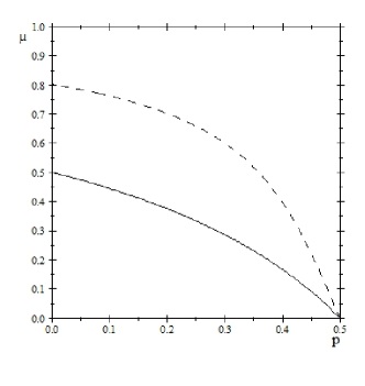
Refer to caption
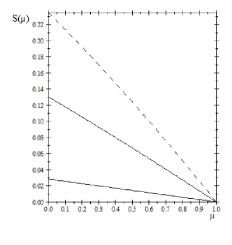
Figure 1: Threshold curves for code effectiveness: concatenated code (dashed line), DFS (solid line). The concatenated code works in the parametric region below the dashed line. The DFS works in the region above the solid line. The repetition code works for any value of μ𝜇\mu when p0.5𝑝0.5p\leq 0.5.

Substituting (47) and (54) into (57), it turns out that the only matrices [RlAk]|𝒞\left[R_{l}A_{k}^{\prime}\right]_{|\mathcal{C}} with non-vanishing trace are given by,

[R1A0]|𝒞=p~0(2)(1001)[R1A3]|𝒞=p~3(2)(1001)\left[R_{1}A_{0}^{\prime}\right]_{|\mathcal{C}}=\sqrt{\tilde{p}_{0}^{\left(2\right)}}\left(\begin{array}[]{cc}1&0\\ 0&1\end{array}\right)\text{, }\left[R_{1}A_{3}^{\prime}\right]_{|\mathcal{C}}=-\sqrt{\tilde{p}_{3}^{\left(2\right)}}\left(\begin{array}[]{cc}1&0\\ 0&1\end{array}\right) (58)

Therefore, the entanglement fidelity DFS(2)(μp)superscriptsubscript𝐷𝐹𝑆2𝜇𝑝\mathcal{F}_{DFS}^{\left(2\right)}\left(\mu\text{, }p\right) defined in (10) results,

DFS(2)(μp)=μ(2p2+2p)+(2p22p+1).superscriptsubscript𝐷𝐹𝑆2𝜇𝑝𝜇2superscript𝑝22𝑝2superscript𝑝22𝑝1.\mathcal{F}_{DFS}^{\left(2\right)}\left(\mu\text{, }p\right)=\mu\left(-2p^{2}+2p\right)+\left(2p^{2}-2p+1\right)\text{.} (59)

We point out that error correction schemes improve the transmission accuracy only if the failure probability 𝒫(μp)𝒫𝜇𝑝\mathcal{P}\left(\mu\text{, }p\right) is strictly less than the error probability p𝑝p gaitan ,

𝒫(μp)=def1(μp)<p.𝒫𝜇𝑝def1𝜇𝑝𝑝.\mathcal{P}\left(\mu\text{, }p\right)\overset{\text{def}}{=}1-\mathcal{F}\left(\mu\text{, }p\right)<p\text{.} (60)

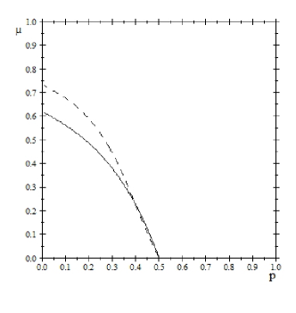
The threshold curves for code effectiveness μ¯(p)¯𝜇𝑝\bar{\mu}\left(p\right) are defined by the relation 1(μ¯(p)p)=01¯𝜇𝑝𝑝01-\mathcal{F}\left(\bar{\mu}\left(p\right)\text{, }p\right)=0. They allow to select the two-dimensional parametric region where error correction schemes are useful. The threshold curve for the DFS for the model appears in Figure 1. The DFS works only in the parametric region above the thin solid line in Figure 1, while the repetition code works for all values of the memory degree μ𝜇\mu when the error probability p𝑝p is less than 0.50.50.5.

Concatenated Code. Following the line of reasoning presented in carloIJQI , we consider the concatenation of the two codes just described. In the case of (16) with n=6𝑛6n=6 qubits and correlated errors in a dephasing quantum channel,

Λ(6)(ρ)=defi1,…, i6=01pi6|i5pi5|i4pi4|i3pi3|i2pi2|i1pi1(Ai6Ai5Ai4Ai3Ai2Ai1)ρ(Ai6Ai5Ai4Ai3Ai2Ai1),superscriptΛ6𝜌defsuperscriptsubscriptsubscript𝑖1,…, subscript𝑖601subscript𝑝conditionalsubscript𝑖6subscript𝑖5subscript𝑝conditionalsubscript𝑖5subscript𝑖4subscript𝑝conditionalsubscript𝑖4subscript𝑖3subscript𝑝conditionalsubscript𝑖3subscript𝑖2subscript𝑝conditionalsubscript𝑖2subscript𝑖1subscript𝑝subscript𝑖1subscript𝐴subscript𝑖6subscript𝐴subscript𝑖5subscript𝐴subscript𝑖4subscript𝐴subscript𝑖3subscript𝐴subscript𝑖2subscript𝐴subscript𝑖1𝜌superscriptsubscript𝐴subscript𝑖6subscript𝐴subscript𝑖5subscript𝐴subscript𝑖4subscript𝐴subscript𝑖3subscript𝐴subscript𝑖2subscript𝐴subscript𝑖1,\Lambda^{(6)}(\rho)\overset{\text{def}}{=}\sum_{i_{1}\text{,..., }i_{6}=0}^{1}p_{i_{6}|i_{5}}p_{i_{5}|i_{4}}p_{i_{4}|i_{3}}p_{i_{3}|i_{2}}p_{i_{2}|i_{1}}p_{i_{1}}\left(A_{i_{6}}A_{i_{5}}A_{i_{4}}A_{i_{3}}A_{i_{2}}A_{i_{1}}\right)\rho\left(A_{i_{6}}A_{i_{5}}A_{i_{4}}A_{i_{3}}A_{i_{2}}A_{i_{1}}\right)^{\dagger}\text{,} (61)

The error superoperator 𝒜𝒜\mathcal{A} associated to channel (61) is defined in terms of the following error operators,

𝒜{A0,.., A63} with Λ(6)(ρ)=defk=0261AkρAk and, k=0261AkAk=I64×64.𝒜superscriptsubscript𝐴0,.., superscriptsubscript𝐴63 with superscriptΛ6𝜌defsuperscriptsubscript𝑘0superscript261superscriptsubscript𝐴𝑘𝜌superscriptsubscript𝐴𝑘 and, superscriptsubscript𝑘0superscript261superscriptsubscript𝐴𝑘superscriptsubscript𝐴𝑘subscript𝐼6464.\mathcal{A}\longleftrightarrow\left\{A_{0}^{\prime}\text{,.., }A_{63}^{\prime}\right\}\text{ with }\Lambda^{(6)}(\rho)\overset{\text{def}}{=}\sum\limits_{k=0}^{2^{6}-1}A_{k}^{\prime}\rho A_{k}^{\prime\dagger}\text{ and, }\sum\limits_{k=0}^{2^{6}-1}A_{k}^{\prime\dagger}A_{k}^{\prime}=I_{64\times 64}\text{.} (62)

The error operators in the Kraus decomposition (62) are k=06(6k)=26=64superscriptsubscript𝑘06binomial6𝑘superscript2664\sum_{k=0}^{6}\binom{6}{k}=2^{6}=64, where (6k)binomial6𝑘\binom{6}{k} is the cardinality of weight-k𝑘k error operators.

We encode our logical qubit with a concatenated subspace obtained by combining the decoherence free subspace in (49) (inner code, 𝒞DFS=𝒞innersubscript𝒞𝐷𝐹𝑆subscript𝒞inner\mathcal{C}_{DFS}=\mathcal{C}_{\text{inner}} ) with the repetition code in (23) (outer code, 𝒞phase=𝒞outersubscript𝒞phasesubscript𝒞outer\mathcal{C}_{\text{phase}}=\mathcal{C}_{\text{outer}}). We obtain that the codewords of the concatenated code 𝒞=𝒞DFS𝒞phase𝒞subscript𝒞𝐷𝐹𝑆subscript𝒞phase\mathcal{C}=\mathcal{C}_{DFS}\circ\mathcal{C}_{\text{phase}} are given by,

|0L=def|+++|1L=def|+++.\left|0_{L}\right\rangle\overset{\text{def}}{=}\left|+++---\right\rangle\text{, }\left|1_{L}\right\rangle\overset{\text{def}}{=}\left|---+++\right\rangle\text{.} (63)

Recall that the detectability condition is given by P𝒞AkP𝒞=λAkP𝒞subscript𝑃𝒞superscriptsubscript𝐴𝑘subscript𝑃𝒞subscript𝜆superscriptsubscript𝐴𝑘subscript𝑃𝒞P_{\mathcal{C}}A_{k}^{\prime}P_{\mathcal{C}}=\lambda_{A_{k}^{\prime}}P_{\mathcal{C}} where the projector operator on the code space 𝒞𝒞\mathcal{C} is P𝒞=|0L0L|+|1L1L|subscript𝑃𝒞ketsubscript0𝐿brasubscript0𝐿ketsubscript1𝐿brasubscript1𝐿P_{\mathcal{C}}=\left|0_{L}\right\rangle\left\langle 0_{L}\right|+\left|1_{L}\right\rangle\left\langle 1_{L}\right|. Observe that,

P𝒞AkP𝒞=0L|Ak|0L|0L0L|+0L|Ak|1L|0L1L|+1L|Ak|0L|1L0L|+1L|Ak|1L|1L1L|.subscript𝑃𝒞superscriptsubscript𝐴𝑘subscript𝑃𝒞quantum-operator-productsubscript0𝐿superscriptsubscript𝐴𝑘subscript0𝐿ketsubscript0𝐿quantum-operator-productsubscript0𝐿quantum-operator-productsubscript0𝐿superscriptsubscript𝐴𝑘subscript1𝐿subscript0𝐿quantum-operator-productsubscript1𝐿quantum-operator-productsubscript1𝐿superscriptsubscript𝐴𝑘subscript0𝐿subscript1𝐿quantum-operator-productsubscript0𝐿quantum-operator-productsubscript1𝐿superscriptsubscript𝐴𝑘subscript1𝐿subscript1𝐿brasubscript1𝐿.P_{\mathcal{C}}A_{k}^{\prime}P_{\mathcal{C}}=\left\langle 0_{L}|A_{k}^{\prime}|0_{L}\right\rangle\left|0_{L}\right\rangle\left\langle 0_{L}\right|+\left\langle 0_{L}|A_{k}^{\prime}|1_{L}\right\rangle\left|0_{L}\right\rangle\left\langle 1_{L}\right|+\left\langle 1_{L}|A_{k}^{\prime}|0_{L}\right\rangle\left|1_{L}\right\rangle\left\langle 0_{L}\right|+\left\langle 1_{L}|A_{k}^{\prime}|1_{L}\right\rangle\left|1_{L}\right\rangle\left\langle 1_{L}\right|\text{.} (64)

Therefore, it turns out that for detectable error operators we must have,

0L|Ak|0L=1L|Ak|1L and, 0L|Ak|1L=1L|Ak|0L=0.quantum-operator-productsubscript0𝐿superscriptsubscript𝐴𝑘subscript0𝐿quantum-operator-productsubscript1𝐿superscriptsubscript𝐴𝑘subscript1𝐿 and, quantum-operator-productsubscript0𝐿superscriptsubscript𝐴𝑘subscript1𝐿quantum-operator-productsubscript1𝐿superscriptsubscript𝐴𝑘subscript0𝐿0.\left\langle 0_{L}|A_{k}^{\prime}|0_{L}\right\rangle=\left\langle 1_{L}|A_{k}^{\prime}|1_{L}\right\rangle\text{ and, }\left\langle 0_{L}|A_{k}^{\prime}|1_{L}\right\rangle=\left\langle 1_{L}|A_{k}^{\prime}|0_{L}\right\rangle=0\text{.} (65)

In the case under consideration, it follows that the only error operator (omitting for the sake of simplicity the proper error amplitudes) not fulfilling the above conditions is proportional to,

Z1Z2Z3Z4Z5Z6.superscript𝑍1superscript𝑍2superscript𝑍3superscript𝑍4superscript𝑍5superscript𝑍6.Z^{1}Z^{2}Z^{3}Z^{4}Z^{5}Z^{6}\text{.} (66)

For such operator, we get

0L|Z1Z2Z3Z4Z5Z6|1L=10 and, 1L|Z1Z2Z3Z4Z5Z6|0L=10 .quantum-operator-productsubscript0𝐿superscript𝑍1superscript𝑍2superscript𝑍3superscript𝑍4superscript𝑍5superscript𝑍6subscript1𝐿10 and, quantum-operator-productsubscript1𝐿superscript𝑍1superscript𝑍2superscript𝑍3superscript𝑍4superscript𝑍5superscript𝑍6subscript0𝐿10 .\left\langle 0_{L}|Z^{1}Z^{2}Z^{3}Z^{4}Z^{5}Z^{6}|1_{L}\right\rangle=1\neq 0\text{ and, }\left\langle 1_{L}|Z^{1}Z^{2}Z^{3}Z^{4}Z^{5}Z^{6}|0_{L}\right\rangle=1\neq 0\text{ .} (67)

Therefore Z1Z2Z3Z4Z5Z6superscript𝑍1superscript𝑍2superscript𝑍3superscript𝑍4superscript𝑍5superscript𝑍6Z^{1}Z^{2}Z^{3}Z^{4}Z^{5}Z^{6} is not detectable. Thus, the cardinality of the set of detectable errors 𝒜detectablesubscript𝒜detectable\mathcal{A}_{\text{detectable}} is 636363. Furthermore, recall that the set of correctable errors 𝒜correctablesubscript𝒜correctable\mathcal{A}_{\text{correctable}} is such that 𝒜correctable𝒜correctablesuperscriptsubscript𝒜correctablesubscript𝒜correctable\mathcal{A}_{\text{correctable}}^{\dagger}\mathcal{A}_{\text{correctable}} is detectable (in the hypothesis of invertible error operators). Therefore, after some reasoning, we conclude that the set of correctable errors is composed by 323232 error operators. The correctable weight-00, 111 and 222 correctable error operators are (omitting the proper error amplitudes),

{I}weight-0{Z1Z2Z3Z4Z5Z6}weight-1subscript𝐼weight-0subscriptsuperscript𝑍1superscript𝑍2superscript𝑍3superscript𝑍4superscript𝑍5superscript𝑍6weight-1\left\{I\right\}_{\text{weight-}0}\text{, }\left\{Z^{1}\text{, }Z^{2}\text{, }Z^{3}\text{, }Z^{4}\text{, }Z^{5}\text{, }Z^{6}\right\}_{\text{weight-}1}\text{, } (68)

and,

{Z1Z2Z1Z3Z1Z4Z1Z5Z1Z6Z2Z3Z2Z4Z2Z5Z2Z6Z3Z4Z3Z5Z3Z6Z4Z5Z4Z6Z5Z6}weight-2,subscriptsuperscript𝑍1superscript𝑍2superscript𝑍1superscript𝑍3superscript𝑍1superscript𝑍4superscript𝑍1superscript𝑍5superscript𝑍1superscript𝑍6superscript𝑍2superscript𝑍3superscript𝑍2superscript𝑍4superscript𝑍2superscript𝑍5superscript𝑍2superscript𝑍6superscript𝑍3superscript𝑍4superscript𝑍3superscript𝑍5superscript𝑍3superscript𝑍6superscript𝑍4superscript𝑍5superscript𝑍4superscript𝑍6superscript𝑍5superscript𝑍6weight-2,\left\{Z^{1}Z^{2}\text{, }Z^{1}Z^{3}\text{, }Z^{1}Z^{4}\text{, }Z^{1}Z^{5}\text{, }Z^{1}Z^{6}\text{, }Z^{2}Z^{3}\text{, }Z^{2}Z^{4}\text{, }Z^{2}Z^{5}\text{, }Z^{2}Z^{6}\text{, }Z^{3}Z^{4}\text{, }Z^{3}Z^{5}\text{, }Z^{3}Z^{6}\text{, }Z^{4}Z^{5}\text{, }Z^{4}Z^{6}\text{, }Z^{5}Z^{6}\right\}_{\text{weight-}2}\text{,} (69)

respectively. The correctable weight-333 errors are,

{Z1Z3Z5Z1Z3Z6Z1Z4Z5Z1Z4Z6Z1Z5Z6Z2Z3Z4Z2Z3Z5Z2Z3Z6Z2Z4Z5Z2Z4Z6}weight-3.subscriptsuperscript𝑍1superscript𝑍3superscript𝑍5superscript𝑍1superscript𝑍3superscript𝑍6superscript𝑍1superscript𝑍4superscript𝑍5superscript𝑍1superscript𝑍4superscript𝑍6superscript𝑍1superscript𝑍5superscript𝑍6superscript𝑍2superscript𝑍3superscript𝑍4superscript𝑍2superscript𝑍3superscript𝑍5superscript𝑍2superscript𝑍3superscript𝑍6superscript𝑍2superscript𝑍4superscript𝑍5superscript𝑍2superscript𝑍4superscript𝑍6weight-3.\left\{Z^{1}Z^{3}Z^{5}\text{, }Z^{1}Z^{3}Z^{6}\text{, }Z^{1}Z^{4}Z^{5}\text{, }Z^{1}Z^{4}Z^{6}\text{, }Z^{1}Z^{5}Z^{6}\text{, }Z^{2}Z^{3}Z^{4}\text{, }Z^{2}Z^{3}Z^{5}\text{, }Z^{2}Z^{3}Z^{6}\text{, }Z^{2}Z^{4}Z^{5}\text{, }Z^{2}Z^{4}Z^{6}\right\}_{\text{weight-}3}\text{.} (70)

There are no weight-444, 555 and 666 correctable error operators. The action of the correctable errors on the codewords in (63) is such that the Hilbert space 26superscriptsubscript26\mathcal{H}_{2}^{6} can be decomposed in two 323232-dimensional orthogonal subspaces 𝒱0Lsuperscript𝒱subscript0𝐿\mathcal{V}^{0_{L}} and 𝒱1Lsuperscript𝒱subscript1𝐿\mathcal{V}^{1_{L}}. In other words, 26=𝒱0L𝒱1Lsuperscriptsubscript26direct-sumsuperscript𝒱subscript0𝐿superscript𝒱subscript1𝐿\mathcal{H}_{2}^{6}=\mathcal{V}^{0_{L}}\oplus\mathcal{V}^{1_{L}} where

𝒱0L=Span{|vk+10L=1p~k(6)Ak|0L} and, 𝒱1L=Span{|vk+11L=1p~k(6)Ak|1L},superscript𝒱subscript0𝐿𝑆𝑝𝑎𝑛ketsuperscriptsubscript𝑣𝑘1subscript0𝐿1superscriptsubscript~𝑝𝑘6superscriptsubscript𝐴𝑘ketsubscript0𝐿 and, superscript𝒱subscript1𝐿𝑆𝑝𝑎𝑛ketsuperscriptsubscript𝑣𝑘1subscript1𝐿1superscriptsubscript~𝑝𝑘6superscriptsubscript𝐴𝑘ketsubscript1𝐿,\mathcal{V}^{0_{L}}=Span\left\{\left|v_{k+1}^{0_{L}}\right\rangle=\frac{1}{\sqrt{\tilde{p}_{k}^{\left(6\right)}}}A_{k}^{\prime}\left|0_{L}\right\rangle\right\}\text{ and, }\mathcal{V}^{1_{L}}=Span\left\{\left|v_{k+1}^{1_{L}}\right\rangle=\frac{1}{\sqrt{\tilde{p}_{k}^{\left(6\right)}}}A_{k}^{\prime}\left|1_{L}\right\rangle\right\}\text{,} (71)

with Ak𝒜correctablesuperscriptsubscript𝐴𝑘subscript𝒜correctableA_{k}^{\prime}\in\mathcal{A}_{\text{correctable}} k=0for-all𝑘0\forall k=0,…, 313131 (numbering the correctable error operators from 00 to 313131). Notice that vkiL|vkjL=δkkδijinner-productsuperscriptsubscript𝑣𝑘subscript𝑖𝐿superscriptsubscript𝑣superscript𝑘subscript𝑗𝐿subscript𝛿𝑘superscript𝑘subscript𝛿𝑖𝑗\left\langle v_{k}^{i_{L}}|v_{k^{\prime}}^{j_{L}}\right\rangle=\delta_{kk^{\prime}}\delta_{ij}, with k𝑘k, k{0,…, 31}superscript𝑘0,…, 31k^{\prime}\in\left\{0\text{,..., }31\right\} and i𝑖i, j{01}𝑗01j\in\left\{0\text{, }1\right\} since,

vkiL|vkjL=iL|Ak1p~k(6)Ak1p~k(6)|jL=1p~k(6)p~k(6)iL|AkAk|jL=1p~k(6)p~k(6)αkkδij=δkkδij,inner-productsuperscriptsubscript𝑣𝑘subscript𝑖𝐿superscriptsubscript𝑣superscript𝑘subscript𝑗𝐿quantum-operator-productsubscript𝑖𝐿superscriptsubscript𝐴𝑘1superscriptsubscript~𝑝𝑘6superscriptsubscript𝐴superscript𝑘1superscriptsubscript~𝑝superscript𝑘6subscript𝑗𝐿1superscriptsubscript~𝑝𝑘6superscriptsubscript~𝑝superscript𝑘6quantum-operator-productsubscript𝑖𝐿superscriptsubscript𝐴𝑘superscriptsubscript𝐴superscript𝑘subscript𝑗𝐿1superscriptsubscript~𝑝𝑘6superscriptsubscript~𝑝superscript𝑘6superscriptsubscript𝛼𝑘superscript𝑘subscript𝛿𝑖𝑗subscript𝛿𝑘superscript𝑘subscript𝛿𝑖𝑗,\left\langle v_{k}^{i_{L}}|v_{k^{\prime}}^{j_{L}}\right\rangle=\left\langle i_{L}|\frac{A_{k-1}^{\prime\dagger}}{\sqrt{\tilde{p}_{k}^{\left(6\right)}}}\frac{A_{k^{\prime}-1}^{\prime}}{\sqrt{\tilde{p}_{k^{\prime}}^{\left(6\right)}}}|j_{L}\right\rangle=\frac{1}{\sqrt{\tilde{p}_{k}^{\left(6\right)}\tilde{p}_{k^{\prime}}^{\left(6\right)}}}\left\langle i_{L}|A_{k}^{\prime\dagger}A_{k^{\prime}}^{\prime}|j_{L}\right\rangle=\frac{1}{\sqrt{\tilde{p}_{k}^{\left(6\right)}\tilde{p}_{k^{\prime}}^{\left(6\right)}}}\alpha_{kk^{\prime}}^{\prime}\delta_{ij}=\delta_{kk^{\prime}}\delta_{ij}\text{,} (72)

where we have used the fact that the square (Hermitian) matrix αkksuperscriptsubscript𝛼𝑘superscript𝑘\alpha_{kk^{\prime}}^{\prime} equals p~k(6)p~k(6)superscriptsubscript~𝑝𝑘6superscriptsubscript~𝑝superscript𝑘6\sqrt{\tilde{p}_{k}^{\left(6\right)}\tilde{p}_{k^{\prime}}^{\left(6\right)}} δkksubscript𝛿𝑘superscript𝑘\delta_{kk^{\prime}}. The recovery superoperator {Rl}subscript𝑅𝑙\mathcal{R}\leftrightarrow\left\{R_{l}\right\} with l=1𝑙1l=1,.., 323232 is defined as knill97 ,

Rl=defVli=01|vliLvliL|,subscript𝑅𝑙defsubscript𝑉𝑙superscriptsubscript𝑖01ketsuperscriptsubscript𝑣𝑙subscript𝑖𝐿brasuperscriptsubscript𝑣𝑙subscript𝑖𝐿,R_{l}\overset{\text{def}}{=}V_{l}\sum_{i=0}^{1}\left|v_{l}^{i_{L}}\right\rangle\left\langle v_{l}^{i_{L}}\right|\text{,} (73)

where the unitary operator Vlsubscript𝑉𝑙V_{l} is such that Vl|vliL=|iLsubscript𝑉𝑙ketsuperscriptsubscript𝑣𝑙subscript𝑖𝐿ketsubscript𝑖𝐿V_{l}\left|v_{l}^{i_{L}}\right\rangle=\left|i_{L}\right\rangle for i{01}𝑖01i\in\left\{0\text{, }1\right\}. Notice that,

Rl=defVli=01|vliLvliL|=|0Lvl0L|+|1Lvl1L|.subscript𝑅𝑙defsubscript𝑉𝑙superscriptsubscript𝑖01ketsuperscriptsubscript𝑣𝑙subscript𝑖𝐿brasuperscriptsubscript𝑣𝑙subscript𝑖𝐿ketsubscript0𝐿brasuperscriptsubscript𝑣𝑙subscript0𝐿ketsubscript1𝐿brasuperscriptsubscript𝑣𝑙subscript1𝐿.R_{l}\overset{\text{def}}{=}V_{l}\sum_{i=0}^{1}\left|v_{l}^{i_{L}}\right\rangle\left\langle v_{l}^{i_{L}}\right|=\left|0_{L}\right\rangle\left\langle v_{l}^{0_{L}}\right|+\left|1_{L}\right\rangle\left\langle v_{l}^{1_{L}}\right|\text{.} (74)

It turns out that the 323232 recovery operators are given by,

Rl+1=R1Alp~l=(|0L0L|+|1L1L|)Alp~l,subscript𝑅𝑙1subscript𝑅1superscriptsubscript𝐴𝑙superscriptsubscript~𝑝𝑙ketsubscript0𝐿brasubscript0𝐿ketsubscript1𝐿brasubscript1𝐿superscriptsubscript𝐴𝑙superscriptsubscript~𝑝𝑙,R_{l+1}=R_{1}\frac{A_{l}^{\prime}}{\sqrt{\tilde{p}_{l}^{\prime}}}=\left(\left|0_{L}\right\rangle\left\langle 0_{L}\right|+\left|1_{L}\right\rangle\left\langle 1_{L}\right|\right)\frac{A_{l}^{\prime}}{\sqrt{\tilde{p}_{l}^{\prime}}}\text{,} (75)

with l{0,…, 31}𝑙0,…, 31l\in\left\{0\text{,..., }31\right\}. Finally, the action of this recovery operation \mathcal{R} on the map Λ(6)(ρ)superscriptΛ6𝜌\Lambda^{\left(6\right)}\left(\rho\right) in (62) leads to,

Λrecover(6)(ρ)(Λ(6))(ρ)=defk=0261l=132(RlAk)ρ(RlAk).superscriptsubscriptΛrecover6𝜌superscriptΛ6𝜌defsuperscriptsubscript𝑘0superscript261superscriptsubscript𝑙132subscript𝑅𝑙superscriptsubscript𝐴𝑘𝜌superscriptsubscript𝑅𝑙superscriptsubscript𝐴𝑘.\Lambda_{\text{recover}}^{\left(6\right)}\left(\rho\right)\equiv\left(\mathcal{R\circ}\Lambda^{(6)}\right)\left(\rho\right)\overset{\text{def}}{=}\sum_{k=0}^{2^{6}-1}\sum\limits_{l=1}^{32}\left(R_{l}A_{k}^{\prime}\right)\rho\left(R_{l}A_{k}^{\prime}\right)^{\dagger}\text{.} (76)

We want to describe the action of Λ(6)superscriptΛ6\mathcal{R\circ}\Lambda^{(6)} restricted to the code subspace 𝒞𝒞\mathcal{C}. Recalling that Al=Alsuperscriptsubscript𝐴𝑙superscriptsubscript𝐴𝑙A_{l}^{\prime}=A_{l}^{\prime\dagger}, it turns out that,

iL|Rl+1Ak|jL=1p~liL|0L0L|AlAk|jL+1p~liL|1L1L|AlAk|jL.quantum-operator-productsubscript𝑖𝐿subscript𝑅𝑙1superscriptsubscript𝐴𝑘subscript𝑗𝐿1superscriptsubscript~𝑝𝑙inner-productsubscript𝑖𝐿subscript0𝐿quantum-operator-productsubscript0𝐿superscriptsubscript𝐴𝑙superscriptsubscript𝐴𝑘subscript𝑗𝐿1superscriptsubscript~𝑝𝑙inner-productsubscript𝑖𝐿subscript1𝐿quantum-operator-productsubscript1𝐿superscriptsubscript𝐴𝑙superscriptsubscript𝐴𝑘subscript𝑗𝐿.\left\langle i_{L}|R_{l+1}A_{k}^{\prime}|j_{L}\right\rangle=\frac{1}{\sqrt{\tilde{p}_{l}^{\prime}}}\left\langle i_{L}|0_{L}\right\rangle\left\langle 0_{L}|A_{l}^{\prime\dagger}A_{k}^{\prime}|j_{L}\right\rangle+\frac{1}{\sqrt{\tilde{p}_{l}^{\prime}}}\left\langle i_{L}|1_{L}\right\rangle\left\langle 1_{L}|A_{l}^{\prime\dagger}A_{k}^{\prime}|j_{L}\right\rangle\text{.} (77)

We now need to compute the 2×2222\times 2 matrix representation [RlAk]|𝒞\left[R_{l}A_{k}^{\prime}\right]_{|\mathcal{C}} of each RlAksubscript𝑅𝑙superscriptsubscript𝐴𝑘R_{l}A_{k}^{\prime} with l=0𝑙0l=0,.., 313131 and k=0𝑘0k=0,.., 261superscript2612^{6}-1 where,

[Rl+1Ak]|𝒞=def(0L|Rl+1Ak|0L0L|Rl+1Ak|1L1L|Rl+1Ak|0L1L|Rl+1Ak|1L).\left[R_{l+1}A_{k}^{\prime}\right]_{|\mathcal{C}}\overset{\text{def}}{=}\left(\begin{array}[]{cc}\left\langle 0_{L}|R_{l+1}A_{k}^{\prime}|0_{L}\right\rangle&\left\langle 0_{L}|R_{l+1}A_{k}^{\prime}|1_{L}\right\rangle\\ \left\langle 1_{L}|R_{l+1}A_{k}^{\prime}|0_{L}\right\rangle&\left\langle 1_{L}|R_{l+1}A_{k}^{\prime}|1_{L}\right\rangle\end{array}\right)\text{.} (78)

For l𝑙l, k=0𝑘0k=0,.., 313131, we note that [Rl+1Ak]|𝒞\left[R_{l+1}A_{k}^{\prime}\right]_{|\mathcal{C}} becomes,

[Rl+1Ak]|𝒞=(0L|AlAk|0L001L|AlAk|1L)=p~lδlk(1001),\left[R_{l+1}A_{k}^{\prime}\right]_{|\mathcal{C}}=\left(\begin{array}[]{cc}\left\langle 0_{L}|A_{l}^{\prime\dagger}A_{k}^{\prime}|0_{L}\right\rangle&0\\ 0&\left\langle 1_{L}|A_{l}^{\prime\dagger}A_{k}^{\prime}|1_{L}\right\rangle\end{array}\right)=\sqrt{\tilde{p}_{l}^{\prime}}\delta_{lk}\left(\begin{array}[]{cc}1&0\\ 0&1\end{array}\right)\text{,} (79)

while for any pair (lk)𝑙𝑘\left(l\text{, }k\right) with l𝑙l =0absent0=0,.., 313131 and k>31𝑘31k>31, it follows that,

0L|Rl+1Ak|0L+1L|Rl+1Ak|1L=0.quantum-operator-productsubscript0𝐿subscript𝑅𝑙1superscriptsubscript𝐴𝑘subscript0𝐿quantum-operator-productsubscript1𝐿subscript𝑅𝑙1superscriptsubscript𝐴𝑘subscript1𝐿0.\left\langle 0_{L}|R_{l+1}A_{k}^{\prime}|0_{L}\right\rangle+\left\langle 1_{L}|R_{l+1}A_{k}^{\prime}|1_{L}\right\rangle=0\text{.} (80)

We conclude that the only matrices [RlAk]|𝒞\left[R_{l}A_{k}^{\prime}\right]_{|\mathcal{C}} with non-vanishing trace are given by [Rl+1Al]|𝒞\left[R_{l+1}A_{l}^{\prime}\right]_{|\mathcal{C}} with l𝑙l =0absent0=0,.., 313131 where,

[Rl+1Al]|𝒞=p~l(1001).\left[R_{l+1}A_{l}^{\prime}\right]_{|\mathcal{C}}=\sqrt{\tilde{p}_{l}^{\prime}}\left(\begin{array}[]{cc}1&0\\ 0&1\end{array}\right)\text{.} (81)

Therefore, the entanglement fidelity conc(6)(μp)superscriptsubscriptconc6𝜇𝑝\mathcal{F}_{\text{conc}}^{\left(6\right)}\left(\mu\text{, }p\right) defined in (10) becomes,

Refer to caption
Figure 2: Threshold curves for code performance: concatenated code vs. DFS (thin solid line) and concatenated code vs. repetition code (dashed line). The concatenated code outperforms the DFS in the parametric region below the solid line and outperforms the repetition code in the region below the dashed line.
conc(6)(μp)superscriptsubscriptconc6𝜇𝑝\displaystyle\mathcal{F}_{\text{conc}}^{\left(6\right)}\left(\mu\text{, }p\right) =p005p0+2p004p10p0+4p003p01p10p0+p003p10p11p0+3p002p01p102p0+absentsuperscriptsubscript𝑝005subscript𝑝02superscriptsubscript𝑝004subscript𝑝10subscript𝑝04superscriptsubscript𝑝003subscript𝑝01subscript𝑝10subscript𝑝0superscriptsubscript𝑝003subscript𝑝10subscript𝑝11subscript𝑝0limit-from3superscriptsubscript𝑝002subscript𝑝01superscriptsubscript𝑝102subscript𝑝0\displaystyle=p_{00}^{5}p_{0}+2p_{00}^{4}p_{10}p_{0}+4p_{00}^{3}p_{01}p_{10}p_{0}+p_{00}^{3}p_{10}p_{11}p_{0}+3p_{00}^{2}p_{01}p_{10}^{2}p_{0}+
+p003p01p10p1+3p002p01p10p11p0+3p00p012p102p0+3p002p012p10p1+p003p01p11p1+superscriptsubscript𝑝003subscript𝑝01subscript𝑝10subscript𝑝13superscriptsubscript𝑝002subscript𝑝01subscript𝑝10subscript𝑝11subscript𝑝03subscript𝑝00superscriptsubscript𝑝012superscriptsubscript𝑝102subscript𝑝03superscriptsubscript𝑝002superscriptsubscript𝑝012subscript𝑝10subscript𝑝1limit-fromsuperscriptsubscript𝑝003subscript𝑝01subscript𝑝11subscript𝑝1\displaystyle+p_{00}^{3}p_{01}p_{10}p_{1}+3p_{00}^{2}p_{01}p_{10}p_{11}p_{0}+3p_{00}p_{01}^{2}p_{10}^{2}p_{0}+3p_{00}^{2}p_{01}^{2}p_{10}p_{1}+p_{00}^{3}p_{01}p_{11}p_{1}+
+p012p103p0+2p00p012p102p1+p00p01p102p11p0+p002p01p10p11p1+p00p01p10p112p0+superscriptsubscript𝑝012superscriptsubscript𝑝103subscript𝑝02subscript𝑝00superscriptsubscript𝑝012superscriptsubscript𝑝102subscript𝑝1subscript𝑝00subscript𝑝01superscriptsubscript𝑝102subscript𝑝11subscript𝑝0superscriptsubscript𝑝002subscript𝑝01subscript𝑝10subscript𝑝11subscript𝑝1limit-fromsubscript𝑝00subscript𝑝01subscript𝑝10superscriptsubscript𝑝112subscript𝑝0\displaystyle+p_{01}^{2}p_{10}^{3}p_{0}+2p_{00}p_{01}^{2}p_{10}^{2}p_{1}+p_{00}p_{01}p_{10}^{2}p_{11}p_{0}+p_{00}^{2}p_{01}p_{10}p_{11}p_{1}+p_{00}p_{01}p_{10}p_{11}^{2}p_{0}+
+2p012p102p11p0+p00p012p10p11p1+p013p102p1.2superscriptsubscript𝑝012superscriptsubscript𝑝102subscript𝑝11subscript𝑝0subscript𝑝00superscriptsubscript𝑝012subscript𝑝10subscript𝑝11subscript𝑝1superscriptsubscript𝑝013superscriptsubscript𝑝102subscript𝑝1.\displaystyle+2p_{01}^{2}p_{10}^{2}p_{11}p_{0}+p_{00}p_{01}^{2}p_{10}p_{11}p_{1}+p_{01}^{3}p_{10}^{2}p_{1}\text{.} (82)

Substituting (22) into (7), we finally get

conc(6)(μp)superscriptsubscriptconc6𝜇𝑝\displaystyle\mathcal{F}_{\text{conc}}^{\left(6\right)}\left(\mu\text{, }p\right) =\displaystyle= μ5(4p5+11p410p3+3p2)+μ4(10p525p4+22p38p2+p)+superscript𝜇54superscript𝑝511superscript𝑝410superscript𝑝33superscript𝑝2limit-fromsuperscript𝜇410superscript𝑝525superscript𝑝422superscript𝑝38superscript𝑝2𝑝\displaystyle\mu^{5}\left(-4p^{5}+\allowbreak 11p^{4}-10p^{3}+3p^{2}\right)+\mu^{4}\left(10p^{5}-25p^{4}+22p^{3}-8p^{2}+p\right)+ (83)
+μ3(6p4+12p37p2+p)+μ2(20p5+58p460p3+25p23p)+superscript𝜇36superscript𝑝412superscript𝑝37superscript𝑝2𝑝limit-fromsuperscript𝜇220superscript𝑝558superscript𝑝460superscript𝑝325superscript𝑝23𝑝\displaystyle+\mu^{3}\left(-6p^{4}+12p^{3}-7p^{2}+p\right)+\mu^{2}\left(-20p^{5}+58p^{4}-60p^{3}\allowbreak+25p^{2}-3p\right)+
+μ(20p553p4+46p313p2)+(6p5+15p410p3+1).𝜇20superscript𝑝553superscript𝑝446superscript𝑝313superscript𝑝26superscript𝑝515superscript𝑝410superscript𝑝31.\displaystyle+\mu\left(20p^{5}-53p^{4}\allowbreak+46p^{3}-13p^{2}\right)+\left(-6p^{5}+15p^{4}-10p^{3}+1\right)\text{.}

The threshold curve for code effectiveness concerning the concatenated code defined in (63) for our noise model appears in Figure 1. It turns out that the concatenated code works in the parametric region below the dashed line.

To uncover the parametric region where one code (say, code-1) outperforms another code (say, code–2), we consider the threshold curves for code performances μ¯(p)¯𝜇𝑝\bar{\mu}\left(p\right) defined by the relation code-1(μ¯(p)p)code-2(μ¯(p)p)=0subscriptcode-1¯𝜇𝑝𝑝subscriptcode-2¯𝜇𝑝𝑝0\mathcal{F}_{\text{code-1}}\left(\bar{\mu}\left(p\right)\text{, }p\right)-\mathcal{F}_{\text{code-2}}\left(\bar{\mu}\left(p\right)\text{, }p\right)=0. We emphasize that in view of equations (45), (59) and (83), it turns out that the concatenated code outperforms the DFS in the parametric region below the solid line (conc(6)(μ¯(p)p)DFS(2)(μ¯(p)p)=0superscriptsubscriptconc6¯𝜇𝑝𝑝superscriptsubscript𝐷𝐹𝑆2¯𝜇𝑝𝑝0\mathcal{F}_{\text{conc}}^{\left(6\right)}\left(\bar{\mu}\left(p\right)\text{, }p\right)-\mathcal{F}_{DFS}^{\left(2\right)}\left(\bar{\mu}\left(p\right)\text{, }p\right)=0) and outperforms the three-qubit repetition code in the region below the dashed line (conc(6)(μ¯(p)p)phase(3)(μ¯(p)p)=0superscriptsubscriptconc6¯𝜇𝑝𝑝superscriptsubscriptphase3¯𝜇𝑝𝑝0\mathcal{F}_{\text{conc}}^{\left(6\right)}\left(\bar{\mu}\left(p\right)\text{, }p\right)-\mathcal{F}_{\text{phase}}^{\left(3\right)}\left(\bar{\mu}\left(p\right)\text{, }p\right)=0) in Figure 2. For the sake of clarity, in Figure 3 we plot the entanglement fidelities (45) (thin solid line), (83) (dashed line) and (59) (thick solid line) for p=102𝑝superscript102p=10^{-2}. Our analysis explicitly shows that none of the two codes (DFS and repetition code) is effective in the extreme limit when the other is, the repetition code still works for correlated errors, whereas the error avoiding code does not work in the absence of correlations. Finally, our final finding leads to conclude that there is a parametric region characterized by intermediate values of the memory parameter where the concatenated code in (63) is particularly advantageous (see Figure 3).
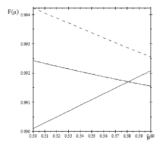
Refer to caption
Figure 3: Entanglement fidelity vs. memory parameter μ𝜇\mu for p=102𝑝superscript102p=10^{-2}: concatenated code (dashed line), DFS (thick solid line) and repetition code (thin solid line).

III.2 Code entropy-based analysis

Repetition code for correlated phase flips. The error correction matrix ΓphasesubscriptΓphase\Gamma_{\text{phase}} for the three-qubit repetition code considered is given by,

Γphase=(p002p00000p00p10p00000p01p10p00000p00p01p1).subscriptΓphasesuperscriptsubscript𝑝002subscript𝑝00000subscript𝑝00subscript𝑝10subscript𝑝00000subscript𝑝01subscript𝑝10subscript𝑝00000subscript𝑝00subscript𝑝01subscript𝑝1.\Gamma_{\text{phase}}=\left(\begin{array}[]{cccc}p_{00}^{2}p_{0}&0&0&0\\ 0&p_{00}p_{10}p_{0}&0&0\\ 0&0&p_{01}p_{10}p_{0}&0\\ 0&0&0&p_{00}p_{01}p_{1}\end{array}\right)\text{.} (84)

Therefore the repetition code entropy 𝒮RC(μp)subscript𝒮RC𝜇𝑝\mathcal{S}_{\text{RC}}\left(\mu\text{, }p\right) results from (14),

𝒮RC=p002p0log2(p002p0)p00p10p0log2(p00p10p0)p01p10p0log2(p01p10p0)p00p01p1log2(p00p01p1),subscript𝒮RCsuperscriptsubscript𝑝002subscript𝑝0subscript2superscriptsubscript𝑝002subscript𝑝0subscript𝑝00subscript𝑝10subscript𝑝0subscript2subscript𝑝00subscript𝑝10subscript𝑝0subscript𝑝01subscript𝑝10subscript𝑝0subscript2subscript𝑝01subscript𝑝10subscript𝑝0subscript𝑝00subscript𝑝01subscript𝑝1subscript2subscript𝑝00subscript𝑝01subscript𝑝1,\mathcal{S}_{\text{RC}}=-p_{00}^{2}p_{0}\log_{2}\left(p_{00}^{2}p_{0}\right)-p_{00}p_{10}p_{0}\log_{2}\left(p_{00}p_{10}p_{0}\right)-p_{01}p_{10}p_{0}\log_{2}\left(p_{01}p_{10}p_{0}\right)-p_{00}p_{01}p_{1}\log_{2}\left(p_{00}p_{01}p_{1}\right)\text{,} (85)

with,

p002p0superscriptsubscript𝑝002subscript𝑝0\displaystyle p_{00}^{2}p_{0} =\displaystyle= μ2(p3+p2)+μ(2p34p2+2p)+(p3+3p23p+1),superscript𝜇2superscript𝑝3superscript𝑝2𝜇2superscript𝑝34superscript𝑝22𝑝superscript𝑝33superscript𝑝23𝑝1,\displaystyle\mu^{2}\left(-p^{3}+p^{2}\right)+\mu\left(2p^{3}-4p^{2}+2p\allowbreak\right)+\left(-p^{3}+3p^{2}-3p+1\right)\text{,}
p00p10p0subscript𝑝00subscript𝑝10subscript𝑝0\displaystyle p_{00}p_{10}p_{0} =\displaystyle= p00p01p1=μ2(p3p2)+μ(2p3+3p2p)+(p32p2+p),subscript𝑝00subscript𝑝01subscript𝑝1superscript𝜇2superscript𝑝3superscript𝑝2𝜇2superscript𝑝33superscript𝑝2𝑝superscript𝑝32superscript𝑝2𝑝,\displaystyle p_{00}p_{01}p_{1}=\mu^{2}\left(p^{3}-p^{2}\right)+\mu\left(-2p^{3}+3p^{2}-p\right)+\left(p^{3}-2p^{2}+\allowbreak p\right)\text{,}
p01p10p0subscript𝑝01subscript𝑝10subscript𝑝0\displaystyle p_{01}p_{10}p_{0} =\displaystyle= μ2(p32p2+p)+μ(2p3+4p22p)+(p32p2+p).superscript𝜇2superscript𝑝32superscript𝑝2𝑝𝜇2superscript𝑝34superscript𝑝22𝑝superscript𝑝32superscript𝑝2𝑝.\displaystyle\mu^{2}\left(\allowbreak p^{3}-2p^{2}+p\right)+\mu\left(-2p^{3}+4p^{2}-\allowbreak 2p\right)+\left(p^{3}-2p^{2}+p\right)\text{.} (86)

In this case it turns out that there is no value of the memory parameter μ𝜇\mu for which 𝒞RCsubscript𝒞RC\mathcal{C}_{\text{RC}} is a unitarily correctable code. In other words, 𝒮RC(μp)0subscript𝒮RC𝜇𝑝0\mathcal{S}_{\text{RC}}\left(\mu\text{, }p\right)\neq 0 for any 0μ10𝜇10\leq\mu\leq 1 with 0p<10𝑝10\leq p<1. Therefore, it never occurs the case where the effort for recovering the code is minimum. For instance, in the extreme limit of μ=1𝜇1\mu=1 it follows that 𝒮RC(μ=1p)=(1p)log2(1p)0subscript𝒮RC𝜇1𝑝1𝑝subscript21𝑝0\mathcal{S}_{\text{RC}}\left(\mu=1\text{, }p\right)=-\left(1-p\right)\log_{2}\left(1-p\right)\neq 0. From Figure 4, we notice that in general in the limit of small error probabilities (p1much-less-than𝑝1p\ll 1), the nearness of 𝒞RCsubscript𝒞𝑅𝐶\mathcal{C}_{RC} to a DFS increases when μ𝜇\mu increases and/or the error probability p𝑝p decreases. Therefore the RC entropy analysis, although not particularly enlightening, confirms that there is no pair of parametric values μ𝜇\mu and p𝑝p for which 𝒞RCsubscript𝒞RC\mathcal{C}_{\text{RC}} provides a fully protected space in the presence of correlated phase-flip errors and the effort required for recovering the quantum state corrupted by the phase-flip noise increases when p𝑝p increases.

Refer to caption
Figure 4: RC entropy vs. μ𝜇\mu for p=2×10²𝑝2superscript102p=2\times 10^{-2} (thick solid line), p=2.5×10²𝑝2.5superscript102p=2.5\times 10^{-2} (thin solid line) and p=3×10²𝑝3superscript102p=3\times 10^{-2} (dash line). The RC entropy does not vanish for μ=1𝜇1\mu=1.

DFS for correlated phase flips. The error correction matrix ΓDFSsubscriptΓDFS\Gamma_{\text{DFS}} for the DFS considered is given by,

ΓDFS=(accb),subscriptΓDFS𝑎𝑐𝑐𝑏,\Gamma_{\text{DFS}}=\left(\begin{array}[]{cc}a&c\\ c&b\end{array}\right)\text{,} (87)

where,

a=defp00p0b=defp11p1c=defp00p0p11p1.𝑎defsubscript𝑝00subscript𝑝0𝑏defsubscript𝑝11subscript𝑝1𝑐defsubscript𝑝00subscript𝑝0subscript𝑝11subscript𝑝1.a\overset{\text{def}}{=}p_{00}p_{0}\text{, }b\overset{\text{def}}{=}p_{11}p_{1}\text{, }c\overset{\text{def}}{=}-\sqrt{p_{00}p_{0}p_{11}p_{1}}\text{.} (88)

Diagonalizing ΛDFSsubscriptΛDFS\Lambda_{\text{DFS}}, it turns out that,

[ΛDFS]diagonal=(λ+00λ),subscriptdelimited-[]subscriptΛDFSdiagonalsubscript𝜆00subscript𝜆,\left[\Lambda_{\text{DFS}}\right]_{\text{diagonal}}=\left(\begin{array}[]{cc}\lambda_{+}&0\\ 0&\lambda_{-}\end{array}\right)\text{,} (89)

with,

λ±=12[(a+b)±(ab)2+4c2].subscript𝜆plus-or-minus12delimited-[]plus-or-minus𝑎𝑏superscript𝑎𝑏24superscript𝑐2.\lambda_{\pm}=\frac{1}{2}\left[\left(a+b\right)\pm\sqrt{\left(a-b\right)^{2}+4c^{2}}\right]\text{.} (90)

Substituting (88) into (90) and recalling that,

p0subscript𝑝0\displaystyle p_{0} =(1p)p1=pp00=((1μ)(1p)+μ),absent1𝑝subscript𝑝1𝑝subscript𝑝001𝜇1𝑝𝜇,\displaystyle=\left(1-p\right)\text{, }p_{1}=p\text{, }p_{00}=\left(\left(1-\mu\right)\left(1-p\right)+\mu\right)\text{, }
p01subscript𝑝01\displaystyle p_{01} =(1μ)(1p)p10=(1μ)pp11=((1μ)p+μ),absent1𝜇1𝑝subscript𝑝101𝜇𝑝subscript𝑝111𝜇𝑝𝜇,\displaystyle=\left(1-\mu\right)\left(1-p\right)\text{, }p_{10}=\left(1-\mu\right)p\text{, }p_{11}=\left(\left(1-\mu\right)p+\mu\right)\text{,} (91)

we obtain,

λ+=μ(2p2+2p)+(2p22p+1) and, λ=0.subscript𝜆𝜇2superscript𝑝22𝑝2superscript𝑝22𝑝1 and, subscript𝜆0.\lambda_{+}=\mu\left(-2p^{2}+2p\right)+\left(2p^{2}-2p+1\right)\text{ and, }\lambda_{-}=0\text{.} (92)

In conclusion the code entropy 𝒮DFS(μp)subscript𝒮DFS𝜇𝑝\mathcal{S}_{\text{DFS}}\left(\mu\text{, }p\right) results from (14),

𝒮DFS(μp)=[μ(2p2+2p)+(2p22p+1)]log2[μ(2p2+2p)+(2p22p+1)].subscript𝒮DFS𝜇𝑝delimited-[]𝜇2superscript𝑝22𝑝2superscript𝑝22𝑝1subscript2𝜇2superscript𝑝22𝑝2superscript𝑝22𝑝1.\mathcal{S}_{\text{DFS}}\left(\mu\text{, }p\right)=-\left[\mu\left(-2p^{2}+2p\right)+\left(2p^{2}-2p+1\right)\right]\log_{2}\left[\mu\left(-2p^{2}+2p\right)+\left(2p^{2}-2p+1\right)\right]\text{.} (93)
Refer to caption
Figure 5: DFS entropy vs. p𝑝p for μ=1𝜇1\mu=1 (thick solid line), μ=0.90𝜇0.90\mu=0.90 (medium solid line), μ=0.75𝜇0.75\mu=0.75 (thin solid line), μ=0.5𝜇0.5\mu=0.5 (thick dash line) and μ=0𝜇0\mu=0 (thin dash line).
Refer to caption
Figure 6: DFS entropy vs. memory parameter for p=101𝑝superscript101p=10^{-1} (dash solid line), p=5×10²𝑝5superscript102p=5\times 10^{-2} (thin solid line) and p=102𝑝superscript102p=10^{-2} (medium solid line). The DFS entropy vanishes for μ=1𝜇1\mu=1.

From Figure 4, it follows that 𝒞DFSsubscript𝒞DFS\mathcal{C}_{\text{DFS}} is a unitarily correctable code only in the extreme limit of μ=1𝜇1\mu=1. In such a case, 𝒮DFS(μ=1p)=0subscript𝒮DFS𝜇1𝑝0\mathcal{S}_{\text{DFS}}\left(\mu=1\text{, }p\right)=0 for any 0p10𝑝10\leq p\leq 1 and thus the effort for recovering the code is minimum since a trivial identity recovery operation will do the job. From Figures 5 and 6, we notice that in general in the limit of small error probabilities (p1much-less-than𝑝1p\ll 1), the effort required for recovering the quantum state corrupted by the phase-flip noise increases when μ𝜇\mu increases and/or p𝑝p increases. Thus, the DFS entropy analysis leads to the conclusion that 𝒞DFSsubscript𝒞DFS\mathcal{C}_{\text{DFS}} provides an especially useful error correction scheme for very small error probabilities and highly correlated phase-flip errors.

Concatenated Code. After some straightforward but tedious algebra, it turns out that the entropy of the concatenated code 𝒮conc.(μp)subscript𝒮conc.𝜇𝑝\mathcal{S}_{\text{conc.}}\left(\mu\text{, }p\right) is given by,

𝒮conc.(μp)=j=031fj(μp)log2fj(μp),subscript𝒮conc.𝜇𝑝superscriptsubscript𝑗031subscript𝑓𝑗𝜇𝑝subscript2subscript𝑓𝑗𝜇𝑝,\mathcal{S}_{\text{conc.}}\left(\mu\text{, }p\right)=-\sum_{j=0}^{31}f_{j}\left(\mu\text{, }p\right)\log_{2}f_{j}\left(\mu\text{, }p\right)\text{,} (94)

where,

f0subscript𝑓0\displaystyle f_{0} =\displaystyle= p005p0f1=f2=p004p10p0f3=f4=f5=f6=p003p01p10p0f7=p003p10p11p0,superscriptsubscript𝑝005subscript𝑝0subscript𝑓1subscript𝑓2superscriptsubscript𝑝004subscript𝑝10subscript𝑝0subscript𝑓3subscript𝑓4subscript𝑓5subscript𝑓6superscriptsubscript𝑝003subscript𝑝01subscript𝑝10subscript𝑝0subscript𝑓7superscriptsubscript𝑝003subscript𝑝10subscript𝑝11subscript𝑝0,\displaystyle p_{00}^{5}p_{0}\text{, }f_{1}=f_{2}=p_{00}^{4}p_{10}p_{0}\text{, }f_{3}=f_{4}=f_{5}=f_{6}=p_{00}^{3}p_{01}p_{10}p_{0}\text{, }f_{7}=p_{00}^{3}p_{10}p_{11}p_{0}\text{,}
f8subscript𝑓8\displaystyle f_{8} =\displaystyle= f9=f10=p002p01p102p0f11=p003p01p10p1f12=f13=f14=p002p01p10p11p0,subscript𝑓9subscript𝑓10superscriptsubscript𝑝002subscript𝑝01superscriptsubscript𝑝102subscript𝑝0subscript𝑓11superscriptsubscript𝑝003subscript𝑝01subscript𝑝10subscript𝑝1subscript𝑓12subscript𝑓13subscript𝑓14superscriptsubscript𝑝002subscript𝑝01subscript𝑝10subscript𝑝11subscript𝑝0,\displaystyle f_{9}=f_{10}=p_{00}^{2}p_{01}p_{10}^{2}p_{0}\text{, }f_{11}=p_{00}^{3}p_{01}p_{10}p_{1}\text{, }f_{12}=f_{13}=f_{14}=p_{00}^{2}p_{01}p_{10}p_{11}p_{0}\text{,}
f15subscript𝑓15\displaystyle f_{15} =\displaystyle= f16=f17=p00p012p102p0f18=f19=f20=p002p012p10p1f21=p003p01p11p1,subscript𝑓16subscript𝑓17subscript𝑝00superscriptsubscript𝑝012superscriptsubscript𝑝102subscript𝑝0subscript𝑓18subscript𝑓19subscript𝑓20superscriptsubscript𝑝002superscriptsubscript𝑝012subscript𝑝10subscript𝑝1subscript𝑓21superscriptsubscript𝑝003subscript𝑝01subscript𝑝11subscript𝑝1,\displaystyle f_{16}=f_{17}=p_{00}p_{01}^{2}p_{10}^{2}p_{0}\text{, }f_{18}=f_{19}=f_{20}=p_{00}^{2}p_{01}^{2}p_{10}p_{1}\text{, }f_{21}=p_{00}^{3}p_{01}p_{11}p_{1}\text{, }
f22subscript𝑓22\displaystyle f_{22} =\displaystyle= p012p103p0f23=f24=p00p012p102p1f25=p00p01p102p11p0f26=p002p01p10p11p1,superscriptsubscript𝑝012superscriptsubscript𝑝103subscript𝑝0subscript𝑓23subscript𝑓24subscript𝑝00superscriptsubscript𝑝012superscriptsubscript𝑝102subscript𝑝1subscript𝑓25subscript𝑝00subscript𝑝01superscriptsubscript𝑝102subscript𝑝11subscript𝑝0subscript𝑓26superscriptsubscript𝑝002subscript𝑝01subscript𝑝10subscript𝑝11subscript𝑝1,\displaystyle p_{01}^{2}p_{10}^{3}p_{0}\text{, }f_{23}=f_{24}=p_{00}p_{01}^{2}p_{10}^{2}p_{1}\text{, }f_{25}=p_{00}p_{01}p_{10}^{2}p_{11}p_{0}\text{, }f_{26}=p_{00}^{2}p_{01}p_{10}p_{11}p_{1}\text{,}
f27subscript𝑓27\displaystyle f_{27} =\displaystyle= p00p01p10p112p0f28=f29=p012p102p11p0f30=p00p012p10p11p1f31=p013p102p1,subscript𝑝00subscript𝑝01subscript𝑝10superscriptsubscript𝑝112subscript𝑝0subscript𝑓28subscript𝑓29superscriptsubscript𝑝012superscriptsubscript𝑝102subscript𝑝11subscript𝑝0subscript𝑓30subscript𝑝00superscriptsubscript𝑝012subscript𝑝10subscript𝑝11subscript𝑝1subscript𝑓31superscriptsubscript𝑝013superscriptsubscript𝑝102subscript𝑝1,\displaystyle p_{00}p_{01}p_{10}p_{11}^{2}p_{0}\text{, }f_{28}=f_{29}=p_{01}^{2}p_{10}^{2}p_{11}p_{0}\text{, }f_{30}=p_{00}p_{01}^{2}p_{10}p_{11}p_{1}\text{, }f_{31}=p_{01}^{3}p_{10}^{2}p_{1}\text{,} (95)

and,

p0subscript𝑝0\displaystyle p_{0} =\displaystyle= (1p)p1=pp00=((1μ)(1p)+μ),1𝑝subscript𝑝1𝑝subscript𝑝001𝜇1𝑝𝜇,\displaystyle\left(1-p\right)\text{, }p_{1}=p\text{, }p_{00}=\left(\left(1-\mu\right)\left(1-p\right)+\mu\right)\text{, }
p01subscript𝑝01\displaystyle p_{01} =\displaystyle= (1μ)(1p)p10=(1μ)pp11=((1μ)p+μ).1𝜇1𝑝subscript𝑝101𝜇𝑝subscript𝑝111𝜇𝑝𝜇.\displaystyle\left(1-\mu\right)\left(1-p\right)\text{, }p_{10}=\left(1-\mu\right)p\text{, }p_{11}=\left(\left(1-\mu\right)p+\mu\right)\text{.} (96)

It can be easily checked that in the extreme limit of μ=1𝜇1\mu=1 it follows that 𝒮conc.(μ=1p)=(1p)log2(1p)0subscript𝒮conc.𝜇1𝑝1𝑝subscript21𝑝0\mathcal{S}_{\text{conc.}}\left(\mu=1\text{, }p\right)=-\left(1-p\right)\log_{2}\left(1-p\right)\neq 0. In general, it appears that results similar to those obtained within the RC code entropy analysis hold (see Figure 7). Then, it seems that the nearness of 𝒞conc.subscript𝒞conc.\mathcal{C}_{\text{conc.}} to a DFS increases when μ𝜇\mu increases and/or the error probability p𝑝p decreases. In particular, the effort required for recovering the quantum state corrupted by the phase-flip noise increases when p𝑝p increases.

Refer to caption
Figure 7: Concatenated code entropy vs. memory parameter μ𝜇\mu for p=101𝑝superscript101p=10^{-1} (dashed solid line), p=5×10²𝑝5superscript102p=5\times 10^{-2} (thin solid line), p=102𝑝superscript102p=10^{-2} (medium solid line),

Our analysis for Model I allows us to conclude that the entanglement fidelity is generally a better code performance quantifier than the code entropy since it is easier to handle computationally and, most of all, it allows to compare performances of different error correction techniques applied to the same error model in a smoother way. However, it appears that the code entropy is especially informative when quantifying the performance of DFSs in the limit of highly correlated and very low error probabilities.

IV Model II: Asymmetric depolarizing noisy quantum memory channel

In this Section, we consider both symmetric and asymmetric depolarizing noisy quantum memory channels and perform quantum error correction via the five qubit stabilizer code 𝒞[[5,1,3]]subscript𝒞delimited-[]513\mathcal{C}_{\left[\left[5,1,3\right]\right]}. We characterize this code by means of the code entropy and the entanglement fidelity as function of the error probability and the degree of memory. In particular, we uncover that while asymmetric depolarizing errors do not affect the entanglement fidelity of the five qubit code, they do affect its code entropy.

IV.1 Entanglement fidelity-based analysis

For the symmetric case, consider five qubits and Markov correlated errors in a depolarizing quantum channel Λ(5)(ρ)superscriptΛ5𝜌\Lambda^{(5)}(\rho),

Λ(5)(ρ)=i1i2i3i4i5=03pi5|i4pi4|i3pi3|i2pi2|i1pi1[Ai5Ai4Ai3Ai2Ai1ρAi1Ai2Ai3Ai4Ai5],superscriptΛ5𝜌superscriptsubscriptsubscript𝑖1subscript𝑖2subscript𝑖3subscript𝑖4subscript𝑖503subscript𝑝conditionalsubscript𝑖5subscript𝑖4subscript𝑝conditionalsubscript𝑖4subscript𝑖3subscript𝑝conditionalsubscript𝑖3subscript𝑖2subscript𝑝conditionalsubscript𝑖2subscript𝑖1subscript𝑝subscript𝑖1delimited-[]subscript𝐴subscript𝑖5subscript𝐴subscript𝑖4subscript𝐴subscript𝑖3subscript𝐴subscript𝑖2subscript𝐴subscript𝑖1𝜌superscriptsubscript𝐴subscript𝑖1superscriptsubscript𝐴subscript𝑖2superscriptsubscript𝐴subscript𝑖3superscriptsubscript𝐴subscript𝑖4superscriptsubscript𝐴subscript𝑖5,\Lambda^{(5)}(\rho)=\sum_{i_{1}\text{, }i_{2}\text{, }i_{3}\text{, }i_{4}\text{, }i_{5}=0}^{3}p_{i_{5}|i_{4}}p_{i_{4}|i_{3}}p_{i_{3}|i_{2}}p_{i_{2}|i_{1}}p_{i_{1}}\left[A_{i_{5}}A_{i_{4}}A_{i_{3}}A_{i_{2}}A_{i_{1}}\rho A_{i_{1}}^{{\dagger}}A_{i_{2}}^{{\dagger}}A_{i_{3}}^{{\dagger}}A_{i_{4}}^{\dagger}A_{i_{5}}^{\dagger}\right]\text{,} (97)

where A0Isubscript𝐴0𝐼A_{0}\equiv I, A1Xsubscript𝐴1𝑋A_{1}\equiv X, A2Ysubscript𝐴2𝑌A_{2}\equiv Y, A3Zsubscript𝐴3𝑍A_{3}\equiv Z are the Pauli operators. The coefficients pil|imsubscript𝑝conditionalsubscript𝑖𝑙subscript𝑖𝑚p_{i_{l}|i_{m}} (conditional probabilities) with l𝑙l, m𝑚m {01,…, 5}absent01,…, 5\in\left\{0\text{, }1\text{,..., }5\right\} satisfy the normalization condition,

i1i2i3i4i5=03pi5|i4pi4|i3pi3|i2pi2|i1pi1=1.superscriptsubscriptsubscript𝑖1subscript𝑖2subscript𝑖3subscript𝑖4subscript𝑖503subscript𝑝conditionalsubscript𝑖5subscript𝑖4subscript𝑝conditionalsubscript𝑖4subscript𝑖3subscript𝑝conditionalsubscript𝑖3subscript𝑖2subscript𝑝conditionalsubscript𝑖2subscript𝑖1subscript𝑝subscript𝑖11.\sum_{i_{1}\text{, }i_{2}\text{, }i_{3}\text{, }i_{4}\text{, }i_{5}=0}^{3}p_{i_{5}|i_{4}}p_{i_{4}|i_{3}}p_{i_{3}|i_{2}}p_{i_{2}|i_{1}}p_{i_{1}}=1\text{.} (98)

For the depolarizing channel Λ(5)(ρ)superscriptΛ5𝜌\Lambda^{(5)}(\rho), coefficients pil|imsubscript𝑝conditionalsubscript𝑖𝑙subscript𝑖𝑚p_{i_{l}|i_{m}} are considered as,

pk|k1=def(1μ)pk+μδk|k1,pk=0=1p,pk=123=p/3.subscript𝑝conditional𝑘𝑘1def1𝜇subscript𝑝𝑘𝜇subscript𝛿conditional𝑘𝑘1,subscript𝑝𝑘01𝑝,subscript𝑝𝑘123𝑝3.p_{k|k-1}\overset{\text{def}}{=}(1-\mu)p_{k}+\mu\delta_{k|k-1}\text{,}\quad p_{k=0}=1-p\text{,}\;p_{k=1\text{, }2\text{, }3}=p/3\text{.} (99)

Following carloPRA , it turns out that the entanglement fidelity symmetric[[5,1,3]](μp)superscriptsubscriptsymmetricdelimited-[]513𝜇𝑝\mathcal{F}_{\text{symmetric}}^{\left[\left[5,1,3\right]\right]}\left(\mu\text{, }p\right) results from (10)

symmetric[[5,1,3]](μp)=k=015fk(μp)=f0+(f1++f6)+(f7++f15),superscriptsubscriptsymmetricdelimited-[]513𝜇𝑝superscriptsubscript𝑘015subscript𝑓𝑘𝜇𝑝subscript𝑓0subscript𝑓1subscript𝑓6subscript𝑓7subscript𝑓15,\mathcal{F}_{\text{symmetric}}^{\left[\left[5,1,3\right]\right]}\left(\mu\text{, }p\right)=\sum\limits_{k=0}^{15}f_{k}\left(\mu\text{, }p\right)=f_{0}+\left(f_{1}+\text{...}+f_{6}\right)+\left(f_{7}+\text{...}+f_{15}\right)\text{,} (100)

where the functions fk(μp)subscript𝑓𝑘𝜇𝑝f_{k}\left(\mu\text{, }p\right) are given by,

f0=p004p0f1==f6=p003p10p0f7==f15=p002p01p10p0,subscript𝑓0superscriptsubscript𝑝004subscript𝑝0subscript𝑓1subscript𝑓6superscriptsubscript𝑝003subscript𝑝10subscript𝑝0subscript𝑓7subscript𝑓15superscriptsubscript𝑝002subscript𝑝01subscript𝑝10subscript𝑝0,f_{0}=p_{00}^{4}p_{0}\text{, }f_{1}=\text{...}=f_{6}=p_{00}^{3}p_{10}p_{0}\text{, }f_{7}=\text{...}=f_{15}=p_{00}^{2}p_{01}p_{10}p_{0}\text{,} (101)

with,

p0subscript𝑝0\displaystyle p_{0} =\displaystyle= 1pp1= p2= p3=p3p00=(1μ)(1p)+μ,1𝑝subscript𝑝1 subscript𝑝2 subscript𝑝3𝑝3subscript𝑝001𝜇1𝑝𝜇,\displaystyle 1-p\text{, }p_{1}=\text{ }p_{2}=\text{ }p_{3}=\frac{p}{3}\text{, }p_{00}=\left(1-\mu\right)\left(1-p\right)+\mu\text{,}
p01subscript𝑝01\displaystyle p_{01} =\displaystyle= p02=p03=(1μ)(1p)p10= p20= p30=p3(1μ).subscript𝑝02subscript𝑝031𝜇1𝑝subscript𝑝10 subscript𝑝20 subscript𝑝30𝑝31𝜇.\displaystyle p_{02}=p_{03}=\left(1-\mu\right)\left(1-p\right)\text{, }p_{10}=\text{ }p_{20}=\text{ }p_{30}=\frac{p}{3}\left(1-\mu\right)\text{.} (102)

For the asymmetric case, we assume that the error probability p𝑝p may be written as,

p=pX+pY+pZ,𝑝subscript𝑝𝑋subscript𝑝𝑌subscript𝑝𝑍,p=p_{X}+p_{Y}+p_{Z}\text{,} (103)

where,

pX=αXppY=αYppZ=αZp,subscript𝑝𝑋subscript𝛼𝑋𝑝subscript𝑝𝑌subscript𝛼𝑌𝑝subscript𝑝𝑍subscript𝛼𝑍𝑝,p_{X}=\alpha_{X}p\text{, }p_{Y}=\alpha_{Y}p\text{, }p_{Z}=\alpha_{Z}p\text{,} (104)

with αX+αY+αZ=1subscript𝛼𝑋subscript𝛼𝑌subscript𝛼𝑍1\alpha_{X}+\alpha_{Y}+\alpha_{Z}=1. Notice that in the symmetric case, we simply have αX=αY=αZ=13subscript𝛼𝑋subscript𝛼𝑌subscript𝛼𝑍13\alpha_{X}=\alpha_{Y}=\alpha_{Z}=\frac{1}{3}. It turns out that the asymmetric[[5,1,3]](μp)superscriptsubscriptasymmetricdelimited-[]513𝜇𝑝\mathcal{F}_{\text{asymmetric}}^{\left[\left[5,1,3\right]\right]}\left(\mu\text{, }p\right) is given by carloPRA ,

asymmetric[[5,1,3]](μpαXαYαZ)=k=015fk(μpαXαYαZ)=f0+(f1++f6)+(f7++f15),superscriptsubscriptasymmetricdelimited-[]513𝜇𝑝subscript𝛼𝑋subscript𝛼𝑌subscript𝛼𝑍superscriptsubscript𝑘015superscriptsubscript𝑓𝑘𝜇𝑝subscript𝛼𝑋subscript𝛼𝑌subscript𝛼𝑍superscriptsubscript𝑓0superscriptsubscript𝑓1superscriptsubscript𝑓6superscriptsubscript𝑓7superscriptsubscript𝑓15,\mathcal{F}_{\text{asymmetric}}^{\left[\left[5,1,3\right]\right]}\left(\mu\text{, }p\text{; }\alpha_{X}\text{, }\alpha_{Y}\text{, }\alpha_{Z}\right)=\sum\limits_{k=0}^{15}f_{k}^{\prime}\left(\mu\text{, }p\text{; }\alpha_{X}\text{, }\alpha_{Y}\text{, }\alpha_{Z}\right)=f_{0}^{\prime}+\left(f_{1}^{\prime}+\text{...}+f_{6}^{\prime}\right)+\left(f_{7}^{\prime}+\text{...}+f_{15}^{\prime}\right)\text{,} (105)

where the functions fk(μpαXαYαZ)superscriptsubscript𝑓𝑘𝜇𝑝subscript𝛼𝑋subscript𝛼𝑌subscript𝛼𝑍f_{k}^{\prime}\left(\mu\text{, }p\text{; }\alpha_{X}\text{, }\alpha_{Y}\text{, }\alpha_{Z}\right) read,

f0superscriptsubscript𝑓0\displaystyle f_{0}^{\prime} =\displaystyle= p004p0f1=p003p0p10f2=p003p0p20f3=p003p0p30f4=p003p01p1f5=p003p01p2f6=p003p01p3,superscriptsubscript𝑝004subscript𝑝0superscriptsubscript𝑓1superscriptsubscript𝑝003subscript𝑝0subscript𝑝10superscriptsubscript𝑓2superscriptsubscript𝑝003subscript𝑝0subscript𝑝20superscriptsubscript𝑓3superscriptsubscript𝑝003subscript𝑝0subscript𝑝30superscriptsubscript𝑓4superscriptsubscript𝑝003subscript𝑝01subscript𝑝1superscriptsubscript𝑓5superscriptsubscript𝑝003subscript𝑝01subscript𝑝2superscriptsubscript𝑓6superscriptsubscript𝑝003subscript𝑝01subscript𝑝3,\displaystyle p_{00}^{4}p_{0}\text{, }f_{1}^{\prime}=p_{00}^{3}p_{0}p_{10}\text{, }f_{2}^{\prime}=p_{00}^{3}p_{0}p_{20}\text{, }f_{3}^{\prime}=p_{00}^{3}p_{0}p_{30}\text{, }f_{4}^{\prime}=p_{00}^{3}p_{01}p_{1}\text{, }f_{5}^{\prime}=p_{00}^{3}p_{01}p_{2}\text{, }f_{6}^{\prime}=p_{00}^{3}p_{01}p_{3}\text{,}
f7superscriptsubscript𝑓7\displaystyle f_{7}^{\prime} =\displaystyle= f8=f9=p002p01p0p10f10=f11=f12=p002p01p0p20f13=f14=f15=p002p01p0p30,superscriptsubscript𝑓8superscriptsubscript𝑓9superscriptsubscript𝑝002subscript𝑝01subscript𝑝0subscript𝑝10superscriptsubscript𝑓10superscriptsubscript𝑓11superscriptsubscript𝑓12superscriptsubscript𝑝002subscript𝑝01subscript𝑝0subscript𝑝20superscriptsubscript𝑓13superscriptsubscript𝑓14superscriptsubscript𝑓15superscriptsubscript𝑝002subscript𝑝01subscript𝑝0subscript𝑝30,\displaystyle f_{8}^{\prime}=f_{9}^{\prime}=p_{00}^{2}p_{01}p_{0}p_{10}\text{, }f_{10}^{\prime}=f_{11}^{\prime}=f_{12}^{\prime}=p_{00}^{2}p_{01}p_{0}p_{20}\text{, }f_{13}^{\prime}=f_{14}^{\prime}=f_{15}^{\prime}=p_{00}^{2}p_{01}p_{0}p_{30}\text{,} (106)

with,

p0subscript𝑝0\displaystyle p_{0} =\displaystyle= 1pp1=αXpp2=αYpp3=αZpp00=(1μ)(1p)+μ,1𝑝subscript𝑝1subscript𝛼𝑋𝑝subscript𝑝2subscript𝛼𝑌𝑝subscript𝑝3subscript𝛼𝑍𝑝subscript𝑝001𝜇1𝑝𝜇,\displaystyle 1-p\text{, }p_{1}=\alpha_{X}p\text{, }p_{2}=\alpha_{Y}p\text{, }p_{3}=\alpha_{Z}p\text{, }p_{00}=\left(1-\mu\right)\left(1-p\right)+\mu\text{,}
p01subscript𝑝01\displaystyle p_{01} =\displaystyle= p02=p03=(1μ)(1p)p10=αXp(1μ)p20=αYp(1μ)p30=αZp(1μ).subscript𝑝02subscript𝑝031𝜇1𝑝subscript𝑝10subscript𝛼𝑋𝑝1𝜇subscript𝑝20subscript𝛼𝑌𝑝1𝜇subscript𝑝30subscript𝛼𝑍𝑝1𝜇.\displaystyle p_{02}=p_{03}=\left(1-\mu\right)\left(1-p\right)\text{, }p_{10}=\alpha_{X}p\left(1-\mu\right)\text{, }p_{20}=\alpha_{Y}p\left(1-\mu\right)\text{, }p_{30}=\alpha_{Z}p\left(1-\mu\right)\text{.} (107)

Recalling that in the symmetric case p1=p2=p3=p3subscript𝑝1subscript𝑝2subscript𝑝3𝑝3p_{1}=p_{2}=p_{3}=\frac{p}{3} and p10=p20=p30=p3(1μ)subscript𝑝10subscript𝑝20subscript𝑝30𝑝31𝜇p_{10}=p_{20}=p_{30}=\frac{p}{3}\left(1-\mu\right) and substituting (107) in (105), it follows that

asymmetric[[5,1,3]](μpαXαYαZ)=symmetric[[5,1,3]](μp).superscriptsubscriptasymmetricdelimited-[]513𝜇𝑝subscript𝛼𝑋subscript𝛼𝑌subscript𝛼𝑍superscriptsubscriptsymmetricdelimited-[]513𝜇𝑝.\mathcal{F}_{\text{asymmetric}}^{\left[\left[5,1,3\right]\right]}\left(\mu\text{, }p\text{; }\alpha_{X}\text{, }\alpha_{Y}\text{, }\alpha_{Z}\right)=\mathcal{F}_{\text{symmetric}}^{\left[\left[5,1,3\right]\right]}\left(\mu\text{, }p\right)\text{.} (108)

Therefore, we conclude that the performance of the five-qubit stabilizer code, when quantified by the entanglement fidelity, remains unaffected by the asymmetry of the depolarizing error probabilities. From (105) it can be shown that such error correction scheme only works for low values of μ𝜇\mu (see Figure 8). Furthermore, it also turns out that the performance of the five qubit quantum stabilizer code is lowered by increasing values of the degree of memory μ𝜇\mu and increasing values of the error probability values p𝑝p (see Figure 9). For a more detailed overview of such findings, we refer to carloPRA .
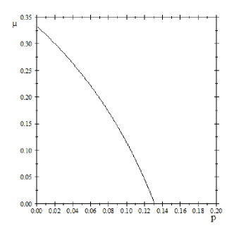
Refer to caption
Figure 8: Threshold curve for the five-qubit stabilizer code effectiveness. The 𝒞[[5,1,3]]subscript𝒞delimited-[]513\mathcal{C}_{\left[\left[5,1,3\right]\right]} code works in the parametric region below the curve.
Refer to caption
Figure 9: [[5,1,3]](μ)superscriptdelimited-[]513𝜇\mathcal{F}^{\left[\left[5,1,3\right]\right]}\left(\mu\right) vs. μ𝜇\mu with 0μ0.330𝜇0.330\leq\mu\leq 0.33 ( for μ>0.33𝜇0.33\mu>0.33, the error correction scheme is not effective anymore) for p=4.50×10²𝑝4.50superscript102p=4.50\times 10^{-2} (thick solid line), p=4.10×10²𝑝4.10superscript102p=4.10\times 10^{-2} (thin solid line) and p=3.75×10²𝑝3.75superscript102p=3.75\times 10^{-2} (dashed line).

IV.2 Code entropy-based analysis

Omitting technical details and following the work presented in the previous Section, it turns out that the five qubit code entropies for the symmetric and asymmetric depolarizing quantum memory channels are given by,

𝒮symmetric[[5,1,3]](μp)=j=015fj(μp)log2fj(μp),superscriptsubscript𝒮symmetricdelimited-[]513𝜇𝑝superscriptsubscript𝑗015subscript𝑓𝑗𝜇𝑝subscript2subscript𝑓𝑗𝜇𝑝,\mathcal{S}_{\text{symmetric}}^{\left[\left[5,1,3\right]\right]}\left(\mu\text{, }p\right)=-\sum_{j=0}^{15}f_{j}\left(\mu\text{, }p\right)\log_{2}f_{j}\left(\mu\text{, }p\right)\text{,} (109)

and,

𝒮asymmetric[[5,1,3]](μpαXαYαZ)=j=015fj(μpαXαYαZ)log2fj(μpαXαYαZ),superscriptsubscript𝒮asymmetricdelimited-[]513𝜇𝑝subscript𝛼𝑋subscript𝛼𝑌subscript𝛼𝑍superscriptsubscript𝑗015superscriptsubscript𝑓𝑗𝜇𝑝subscript𝛼𝑋subscript𝛼𝑌subscript𝛼𝑍subscript2superscriptsubscript𝑓𝑗𝜇𝑝subscript𝛼𝑋subscript𝛼𝑌subscript𝛼𝑍,\mathcal{S}_{\text{asymmetric}}^{\left[\left[5,1,3\right]\right]}\left(\mu\text{, }p\text{; }\alpha_{X}\text{, }\alpha_{Y}\text{, }\alpha_{Z}\right)=-\sum_{j=0}^{15}f_{j}^{\prime}\left(\mu\text{, }p\text{; }\alpha_{X}\text{, }\alpha_{Y}\text{, }\alpha_{Z}\right)\log_{2}f_{j}^{\prime}\left(\mu\text{, }p\text{; }\alpha_{X}\text{, }\alpha_{Y}\text{, }\alpha_{Z}\right)\text{,} (110)

respectively. The explicit expressions for the functions fj(μp)subscript𝑓𝑗𝜇𝑝f_{j}\left(\mu\text{, }p\right) and fj(μpαXαYαZ)superscriptsubscript𝑓𝑗𝜇𝑝subscript𝛼𝑋subscript𝛼𝑌subscript𝛼𝑍f_{j}^{\prime}\left(\mu\text{, }p\text{; }\alpha_{X}\text{, }\alpha_{Y}\text{, }\alpha_{Z}\right) are given in (101) and (106), respectively. From (109) and (110), it can be shown that

𝒮symmetric[[5,1,3]](μp)𝒮asymmetric[[5,1,3]](μpαXαYαZ).superscriptsubscript𝒮symmetricdelimited-[]513𝜇𝑝superscriptsubscript𝒮asymmetricdelimited-[]513𝜇𝑝subscript𝛼𝑋subscript𝛼𝑌subscript𝛼𝑍.\mathcal{S}_{\text{symmetric}}^{\left[\left[5,1,3\right]\right]}\left(\mu\text{, }p\right)\neq\mathcal{S}_{\text{asymmetric}}^{\left[\left[5,1,3\right]\right]}\left(\mu\text{, }p\text{; }\alpha_{X}\text{, }\alpha_{Y}\text{, }\alpha_{Z}\right)\text{.} (111)

Numerical evidence of the disequality in (111) can be easily verified at least for a suitable choice of model parameters μ𝜇\mu, αXsubscript𝛼𝑋\alpha_{X}, αYsubscript𝛼𝑌\alpha_{Y} and αZsubscript𝛼𝑍\alpha_{Z}. In Figure 10, we plot the change of the five qubit code entropy Δ𝒮(p)subscriptΔ𝒮𝑝\Delta_{\mathcal{S}}\left(p\right) as function of the error probability p𝑝p. Specifically, Δ𝒮(p)subscriptΔ𝒮𝑝\Delta_{\mathcal{S}}\left(p\right) is the difference between the five qubit code entropies 𝒮symmetric[[5,1,3]](p)superscriptsubscript𝒮symmetricdelimited-[]513𝑝\mathcal{S}_{\text{symmetric}}^{\left[\left[5,1,3\right]\right]}\left(p\right) and 𝒮asymmetric[[5,1,3]](p)superscriptsubscript𝒮asymmetricdelimited-[]513𝑝\mathcal{S}_{\text{asymmetric}}^{\left[\left[5,1,3\right]\right]}\left(p\right) in the absence of correlations (μ=0𝜇0\mu=0) with αx=αy=14subscript𝛼𝑥subscript𝛼𝑦14\alpha_{x}=\alpha_{y}=\frac{1}{4} and αz=12subscript𝛼𝑧12\alpha_{z}=\frac{1}{2}. The positivity of Δ𝒮(p)subscriptΔ𝒮𝑝\Delta_{\mathcal{S}}\left(p\right) leads to conclude that when the error model considered is defined by a suitable choice of numerical values of the model parameters, it can happen that the effort required for recovering the five qubit code in the asymmetric case is less than in the symmetric case. This scenario never occurs when quantifying the performance of the five qubit code applied to asymmetric and correlated depolarizing errors by means of the entanglement fidelity.
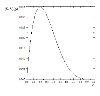
Refer to caption
Figure 10: Difference between the five qubit stabilizer code entropies 𝒮symmetric[[5,1,3]](p)superscriptsubscript𝒮symmetricdelimited-[]513𝑝\mathcal{S}_{\text{symmetric}}^{\left[\left[5,1,3\right]\right]}\left(p\right) and 𝒮asymmetric[[5,1,3]](p)superscriptsubscript𝒮asymmetricdelimited-[]513𝑝\mathcal{S}_{\text{asymmetric}}^{\left[\left[5,1,3\right]\right]}\left(p\right) in the absence of correlations (μ=0𝜇0\mu=0) with αx=αy=14subscript𝛼𝑥subscript𝛼𝑦14\alpha_{x}=\alpha_{y}=\frac{1}{4} and αz=12subscript𝛼𝑧12\alpha_{z}=\frac{1}{2}.

From an analytical point of view, (111) can be readily understood by noticing that 𝒮symmetric[[5,1,3]](μp)superscriptsubscript𝒮symmetricdelimited-[]513𝜇𝑝\mathcal{S}_{\text{symmetric}}^{\left[\left[5,1,3\right]\right]}\left(\mu\text{, }p\right) in (109) and 𝒮asymmetric[[5,1,3]](μpαXαYαZ)superscriptsubscript𝒮asymmetricdelimited-[]513𝜇𝑝subscript𝛼𝑋subscript𝛼𝑌subscript𝛼𝑍\mathcal{S}_{\text{asymmetric}}^{\left[\left[5,1,3\right]\right]}\left(\mu\text{, }p\text{; }\alpha_{X}\text{, }\alpha_{Y}\text{, }\alpha_{Z}\right) in (110) are sums of terms that are nonlinear in the functions (amplitude square probabilities of the correctable error operators) fj(μp)subscript𝑓𝑗𝜇𝑝f_{j}\left(\mu\text{, }p\right) and fj(μpαXαYαZ)superscriptsubscript𝑓𝑗𝜇𝑝subscript𝛼𝑋subscript𝛼𝑌subscript𝛼𝑍f_{j}^{\prime}\left(\mu\text{, }p\text{; }\alpha_{X}\text{, }\alpha_{Y}\text{, }\alpha_{Z}\right), respectively. As a matter of fact it turns out that,

k=015fk=k=015fk,superscriptsubscript𝑘015subscript𝑓𝑘superscriptsubscript𝑘015superscriptsubscript𝑓𝑘,\sum_{k=0}^{15}f_{k}=\sum_{k=0}^{15}f_{k}^{\prime}\text{,} (112)

with f0=f0=p004p0superscriptsubscript𝑓0subscript𝑓0superscriptsubscript𝑝004subscript𝑝0f_{0}^{\prime}=f_{0}=p_{00}^{4}p_{0}, f1++f6=f1++f6superscriptsubscript𝑓1superscriptsubscript𝑓6subscript𝑓1subscript𝑓6f_{1}^{\prime}+...+f_{6}^{\prime}=f_{1}+...+f_{6}, f7++f15=f7++f15superscriptsubscript𝑓7superscriptsubscript𝑓15subscript𝑓7subscript𝑓15f_{7}^{\prime}+...+f_{15}^{\prime}=f_{7}+...+f_{15} and, fifjsuperscriptsubscript𝑓𝑖superscriptsubscript𝑓𝑗f_{i}^{\prime}\neq f_{j}^{\prime} for i𝑖i, j=1𝑗1j=1,…, 666; f7=f8=f9=p002p01p0p10superscriptsubscript𝑓7superscriptsubscript𝑓8superscriptsubscript𝑓9superscriptsubscript𝑝002subscript𝑝01subscript𝑝0subscript𝑝10f_{7}^{\prime}=f_{8}^{\prime}=f_{9}^{\prime}=p_{00}^{2}p_{01}p_{0}p_{10}; f10=f11=f12=p002p01p0p20superscriptsubscript𝑓10superscriptsubscript𝑓11superscriptsubscript𝑓12superscriptsubscript𝑝002subscript𝑝01subscript𝑝0subscript𝑝20f_{10}^{\prime}=f_{11}^{\prime}=f_{12}^{\prime}=p_{00}^{2}p_{01}p_{0}p_{20} and f13=f14=f15=p002p01p0p30superscriptsubscript𝑓13superscriptsubscript𝑓14superscriptsubscript𝑓15superscriptsubscript𝑝002subscript𝑝01subscript𝑝0subscript𝑝30f_{13}^{\prime}=f_{14}^{\prime}=f_{15}^{\prime}=p_{00}^{2}p_{01}p_{0}p_{30}. However, the constraint in (112) together with the nonlinearity in f𝑓f and fsuperscript𝑓f^{\prime} characterizing the expressions of the code entropies in (109) and (110) imply that,

k=015fklog2fkk=015fklog2fk.superscriptsubscript𝑘015subscript𝑓𝑘subscript2subscript𝑓𝑘superscriptsubscript𝑘015superscriptsubscript𝑓𝑘subscript2superscriptsubscript𝑓𝑘.\sum_{k=0}^{15}f_{k}\log_{2}f_{k}\neq\sum_{k=0}^{15}f_{k}^{\prime}\log_{2}f_{k}^{\prime}\text{.} (113)

In conclusion, since the entanglement fidelity is a linear combination of the amplitude square probabilities of the correctable error operators, Eq. (112) holds true, and the equality in (108) is proven. On the contrary, the code entropy is a nonlinear combination of the amplitude square probabilities and the use of (113) leads naturally to the inequality in (111).

Therefore, we conclude that the performance of the five-qubit stabilizer code, when quantified by the code entropy and not by the entanglement fidelity, does remain affected by the asymmetry of the depolarizing error probabilities. Our finding provides a neat quantitative manifestation of the conceptual fact kribs that no single code performance quantifier holds all the information on a code.

V Final Remarks

In this article, we studied the properties of error correcting codes for noise models in the presence of asymmetries and/or correlations by means of the entanglement fidelity and the code entropy. We considered a dephasing Markovian memory channel (Model I) and both symmetric and asymmetric depolarizing quantum memory channels (Model II). For each model, we presented both an entanglement fidelity-based and a code entropy-based analyses. For Model I, we used three codes: the repetition code 𝒞RCsubscript𝒞𝑅𝐶\mathcal{C}_{RC}, the DFS 𝒞DFSsubscript𝒞𝐷𝐹𝑆\mathcal{C}_{DFS} and the concatenated code 𝒞DFS𝒞RCsubscript𝒞𝐷𝐹𝑆subscript𝒞𝑅𝐶\mathcal{C}_{DFS}\circ\mathcal{C}_{RC}. For Model II, we employed the five qubit stabilizer code 𝒞[[5,1,3]]subscript𝒞delimited-[]513\mathcal{C}_{\left[\left[5,1,3\right]\right]}.

For Model I, the entanglement fidelity-based analysis allows to find out the parametric regions where the chosen error correction schemes are effective (see Figure 1). This analysis is also suitable to determine where, within such parametric regions, one code outperforms the other (see Figure 2). In particular, we showed that the concatenated code quantified by the entanglement fidelity is useful to combat partially correlated phase-flip errors (see Figure 3). The code entropy-based analysis for Model I leads to the conclusion that the effort required for recovering the quantum state corrupted by correlated phase-flip errors increases when the memory parameter μ𝜇\mu decreases and the error probability p𝑝p increases (see Figures 4 and 6). Furthermore, it turns out that only 𝒞DFSsubscript𝒞𝐷𝐹𝑆\mathcal{C}_{DFS} is a unitarily correctable code for the noise model considered in the limiting case of μ=1𝜇1\mu=1 (see Figure 5). When applied to the concatenated code, the code entropy-based analysis is not as enlightening as the entanglement-fidelity based analysis. It is not particularly useful for drawing performance comparisons with the repetition code (see Figure 7).

For Model II, the entanglement fidelity-based analysis allows us to find out that the five qubit stabilizer code only works for small values of μ𝜇\mu (see Figure 8). Furthermore, the performance of this code applied to symmetric and asymmetric correlated depolarizing errors is lowered by increasing values of the memory parameter μ𝜇\mu and increasing values of the error probability p𝑝p (see Figure 9). Finally, the code entropy-based analysis applied to Model II leads to an interesting result. While asymmetry in the depolarizing errors does not affect in any case the performance of the five qubit stabilizer code quantified by means of the entanglement fidelity, it may affect positively the performance of 𝒞[[5,1,3]]subscript𝒞delimited-[]513\mathcal{C}_{\left[\left[5,1,3\right]\right]} by lowering the effort required for recovering the code subjected to asymmetric depolarizing errors (see Figure 10).

Although our work is limited to only few error models in the presence of correlations and asymmetry and we only perform error correction by means of few quantum codes, we feel we have gathered enough evidence to draw the following conclusions on the code performance quantifiers employed: a) while the code entropy may capture new undetected features of a code with respect to those encoded into the entanglement fidelity and deserves further investigations, it is certainly harder to compute for realistic physical models and non-trivial quantum codes; b) the code entropy seems to lack the reliability and practicality characterizing the entanglement fidelity.

In summary, the entropy of a code appears to be an interesting auxiliary tool for quantifying the code performances. In particular, it is our intention to explore in future investigations the possibility of devising a hybrid code performance quantifier whose nonlinear structure in the amplitude square probabilities of the correctable error operators may not be necessarily characterized by the logarithmic behavior which identifies the code entropy. For the time being, motivated by our analysis and in agreement with nielsen-fidel ; cory ; knill-exp , we believe that the entanglement fidelity remains the most relevant tool to maximize in schemes for quantum error correction.

Acknowledgements.
The research leading to these results has received funding from the European Commission’s Seventh Framework Programme (FP7/2007–2013) under grant agreements no. 213681.

References

  • (1) Gottesman, D., An Introduction to Quantum Error Correction and Fault-Tolerant Quantum Computation, in Quantum Information Science and Its Contributions to Mathematics, Proceedings of Symposia in Applied Mathematics, Amer. Math. Soc., Providence, Rhode Island, 2010, 13-58.
  • (2) Lidar, D. A. and Whaley, K. B., Decoherence-Free Subspaces and Subsystems, in: F. Benatti and R. Floreanini, (eds.), Irreversible Quantum Dynamics, Springer Lecture Notes in Physics, Berlin, 2003, 83-120.
  • (3) Garg, A., Phys. Rev. Lett. 77 (1996), 964.
  • (4) Loss, D. and Di Vincenzo, D. P., Phys. Rev. A 57 (1998), 120.
  • (5) Hwang, W. Y., Ahn, D. and Hwang, S. W., Phys. Rev. A 63 (2001), 022303.
  • (6) Clemens, J. P., Siddiqui, S. and Gea-Banacloche, J., Phys. Rev. A 69 (2004), 062313.
  • (7) Klesse, R. and Frank, S., Phys. Rev. Lett. 95 (2005), 230503.
  • (8) Shabani, A. Phys. Rev. A 77 (2008), 022323.
  • (9) D’Arrigo, A., De Leo, E., Benenti, G., Falci, G., Int. J. Quantum Inf. 6 (2008), 651.
  • (10) Cafaro, C. and Mancini, S., Phys. Lett. A 374 (2010), 2688.
  • (11) Cafaro, C. and Mancini, S., Phys. Rev. A 82 (2010), 012306.
  • (12) Astafiev, O., Pashkin, Yu. A., Nakamura, Y., Yamamoto, T. and Tsai, J. S., Phys. Rev. Lett. 93 (2004), 267007.
  • (13) Ioffe, L. and Mezard, M. Phys. Rev. A 75 (2007), 032345.
  • (14) Evans, Z. W. E., Stephens, A. M., Cole, J. H., Hollenberg, L. C. L., arXiv:quant-ph/0709.3875 (2007).
  • (15) Stephens, A. M., Evans, Z. W. E., Devitt, S. J. and Hollenberg, L. C. L. Phys. Rev. A 77 (2008), 062335.
  • (16) Sarvepalli, P. K., Roetteler, M., Klappenecker, A., arXiv:quant-ph/0804.4316 (2008).
  • (17) Aly, S. A., arXiv:quant-ph/0803.0764 (2008).
  • (18) Gottesman, D., arXiv:quant-ph/9607027 (1996).
  • (19) Calderbank, R. A., Rains, E., Shor, P. and Sloane, N., IEEE Trans. Inf. Theor. 44 (1998), 1369.
  • (20) Forney, G. D. Jr., Concatenated Codes, MIT Press, Cambridge, 1966.
  • (21) Gottesman, D., Stabilizer codes and quantum error correction, Caltech Ph.D. Thesis (1997), arXiv:quant-ph/9705052.
  • (22) Knill, E. and Laflamme, R., arXiv:quant-ph/9608012 (1996).
  • (23) Nielsen, M. A. and Chuang, I. L. Quantum Computation and Information, Cambridge University Press, Cambridge, 2000.
  • (24) Nielsen, M. A., arXiv: quant-ph/9606012 (1996).
  • (25) Schumacher, B., Phys. Rev. A 54 (1996), 2615.
  • (26) Kribs, D.W., Pasieka, A., Zyczkowski, K., Open Syst. Inf. Dyn. 15 (2008), 329.
  • (27) Majgier, K., Maassen, H., Zyczkowski, K., Quantum Inf. Process. 3 (2010), 343.
  • (28) Lindblad, G., Quantum entropy and quantum measurements, Lecture Notes in Physics 378 (1991), 36.
  • (29) Kaye, P., Laflamme R., Mosca, M., An Introduction to Quantum Computing, Oxford University Press, Oxford, 2007.
  • (30) Knill, E., Laflamme, R., Ashikhmin, A., Barnum, H., Viola, L., Zurek, W.H., arXiv:quant-ph/020717 (2002).
  • (31) Knill, E. and Laflamme, R., Phys. Rev. A 55 (1997), 900.
  • (32) Gaitan, F., Quantum Error Correction and Fault Tolerant Quantum Computing, CRC Press, 2008.
  • (33) Cafaro, C. and Mancini, S., arXiv:quant-ph/1006.2051 (2010).
  • (34) Cory, D., Price, M. D., Maas, W., Knill, E., Laflamme, R., Zurek, W. H., Havel, T. F. and Somaroo, S. S., Phys. Rev. Lett. 81 (1998), 2152.
  • (35) Knill, E., Laflamme, R., Martinez, R. and Negrevergne, C., Phys. Rev. Lett. 86 (2001), 5811.