Three-body structure of low-lying ¹⁸Ne states

Abstract

We investigate to what extent ¹⁸Ne can be descibed as a three-body system made of an inert ¹⁶O-core and two protons. We compare to experimental data and occasionally to shell model results. We obtain three-body wave functions with the hyperspherical adiabatic expansion method. We study the spectrum of ¹⁸Ne, the structure of the different states and the predominant transition strengths. Two $0^{+}$, two $2^{+}$, and one $4^{+}$ bound states are found where they are all known experimentally. Also one $3^{+}$ close to threshold is found and several negative parity states, $1^{-}$, $3^{-}$, $0^{-}$, $2^{-}$, most of them bound with respect to the ¹⁶O excited $3^{-}$ state. The structures are extracted as partial wave components, as spatial sizes of matter and charge, and as probability distributions. Electromagnetic decay rates are calculated for these states. The dominating decay mode for the bound states is $E2$ and occasionally also $M1$.

1 Introduction

Nuclear cluster structures appear in various disguises especially in light nuclei. The cluster constituents are often nucleons and $\alpha$-particles, possibly combined with a core-nucleus. These structures, which appear both as ground and excited (resonance) states, are sometimes well described as three-body systems. The conventional wisdom is that prominent clusters are most likely to appear close to the threshold energy for fragmentation into the cluster constituents. This implies that cluster structures for ordinary bound nuclei are more likely to appear in excited states than in ground states, except for dripline nuclei where the ground state is close to the nucleon threshold and dominating one or two-nucleon structures appear jen04 ; tho04 ; fre07 ; bla08 .

Well-known three-body examples are the first $0^{+}$ resonance in ¹²C alv07 , the lowest $0^{+}$ and $2^{+}$ states in ⁶He, ⁶Be and ⁶Li gar06 , the $3/2^{-}$ ground state in ¹¹Li gar01 , three excited bound states in ¹²Be rom08 , the ground state and four resonances in ¹⁷Ne gar03 , the ground state and several resonances in ⁹Be alv08 , and three resonances in ⁵H die07 . Other nuclear states have significant admixtures of non-cluster structure (¹²C($2^{\pm}$)) alv08a while some states are far better described without any cluster structure (¹²C($1^{\pm}$)) alv07 . One line of investigation is to carry out the three-body computation for a given system and compare the computed observables with known measured values and then predict others.

If the computed bulk structure of a nuclear state matches measurements the description is an immediate success. However, even for cases where no traces of any three-body structure can be found the computation can be considered a necessary ingredient to describe the three-body decay of an underlying many-body resonance, examples are ¹²C($1^{\pm})$ alv08b . Resonances decaying into three clusters are now investigated accurately in details in complete kinematics fyn04 . Both structure and dynamic evolution from small to large distances are important in a description of the momentum distributions of the decay products. A few such decaying structures have been investigated theoretically and compared to available data gar06b ; alv08 .

Recently the decay products, two protons and ¹⁶O, from the 6.15 MeV $1^{-}$ state in ¹⁸Ne was measured gom01 ; ras08 . In the same nucleus the 4.522 MeV $1^{-}$ state received attention as a doorway state to produce the water molecule bel01 which has the same number of neutrons, protons and electrons as the ¹⁸Ne-atom. Also the first 3⁺ state of this nucleus plays an important role in astrophysics related to the abundance ratio between ¹⁸F and ¹⁷F bar00 . The ¹⁷F$(p,\gamma)^{18}$Ne cross section has been investigated in a two-cluster coupled-channel model duf04 , and recently also measured directly chi09 . The first question in this connection is obviously which structures have these, and perhaps other, ¹⁸Ne states. The low-energy spectrum of ¹⁸Ne is typical for a quadrupole vibration with an equidistant spacing between $0^{+}$, $2^{+}$, and a triplet of $0^{+},2^{+},4^{+}$ states til95 . Still higher at and above the two-proton threshold a $0^{+}$ and a $3^{+}$ appear with a number of other states without an obvious recognizable pattern, see Fig.1.

Figure 1: Measured spectra compared to computations with the interactions I,II,III (see text and table 1) relating to the $0^{+}$ ground state of the core and IV relates to the $3^{-}$ core excitation. The threshold of $E=0$ corresponds to infinite zero separation of the two protons and the oxygen core.

The different states may originate from separate structures described for example as vibrations, single-particle excitations, pairing correlations, or obtained in combinations of even more complicated few or many-body features. In particular the coupled two-body cluster model provides one type of structure information duf04 . Also a number of interacting shell model calculations have provided structure information about the low-lying excited states of the $A=18$ isobaric system, ¹⁸O ¹⁸F ¹⁸Ne, see e.g. she98 ; bro02 . The results are in general that many of the states are more complicated than two nucleons and the ¹⁶O-core. This is not surprising when the excitation energy is sufficiently large to accomodate core excitations. However, the shell model is designed to describe spatially confined bound state structures without strong cluster configurations beyond the chosen core-valence division. This means that large-distance structures are inaccessible or inaccurate in shell model calculations. This applies in particular to resonances and doorway states in reactions.

Specifically, three-body decays of resonances cannot be described by two-body cluster or shell models. The resonance structures necessarily change from the many-body short-distance behavior to three-body clusters at intermediate distances. In addition, the two-body structure is inadequate and the three-body structure itself often change dramatically from intermediate to large distances alv07 ; gar06 ; alv08 ; alv08a . The three-body structures must be accurately described to meet requirements of up-to-date measurements. In other words shell model calculations necessarily must be supplemented by few-body calculations as provided in the present paper.

To clear the road towards computing the three-body decays measured in gom01 ; ras08 we start with assuming few-body structures to see how far this will bring us in a quantitative description of the various states. Since ¹⁷Ne (¹⁵O+p+p) is Borromean an extra neutron suggest a four-body structure but a neutron and ¹⁵O form a strongly bound doubly magic nucleus, ¹⁶O, and a three-body structure of ¹⁶O+p+p is probably a better starting point. Unfortunately it is then unlikely that the $1^{-}$ states simultaneously are simple three-body structures maintaining an ¹⁶O ground state core. At least the $3^{-}$ state in the ¹⁶O core til95 can be expected to contribute.

In the present paper we attempt to describe the low-lying (bound and resonance) states in ¹⁸Ne as three-body states. If possible this is a huge simplification from the full problem of 18 interacting nucleons. These investigations are a generalization of the classical nucleon-core model and its extension to two mutually interacting particles occupying single-particle levels provided by a core but without additional nucleon-core interaction. In any case, the results are a prerequisite for description of three-body decaying resonances like the measured $1^{-}$ state ras08 ; gom01 . The paper is organized as follows. In section 2 we briefly describe the notation by sketching the three-body method and the constraints used to determine the crucial two-body interactions. The structures are shown in section 3, and the sizes and electromagnetic transitions are given in 4. Finally, section 5 contains a summary and the conclusions.

2 Method and interactions

The principal model assumption is that ¹⁸Ne can be described as a three-body system made by a ¹⁶O core and two protons. The wave functions for the different bound states are obtained with the hyperspherical adiabatic expansion method. A detailed description of the method can be found in nie01 .

2.1 Theoretical formulation

This method solves the Faddeev equations in coordinate space. The wave functions are computed as a sum of three Faddeev components $\psi^{(i)}(\mbox{\boldmath$x$}_{i},\mbox{\boldmath$y$}_{i})$ ($i$=1,2,3), each of them expressed in one of the three possible sets of Jacobi coordinates $\{\mbox{\boldmath$x$}_{i},\mbox{\boldmath$y$}_{i}\}$. Each component is then expanded in terms of a complete set of angular functions $\{\phi_{n}^{(i)}\}$

$$\psi^{(i)}={1\over\rho^{5/2}}\sum_{n}f_{n}(\rho)\phi_{n}^{(i)}(\rho,\Omega_{i});(\Omega_{i}\equiv\{\alpha_{i},\Omega_{x_{i}},\Omega_{y_{i}}\}),$$ (1)

where $\rho=\sqrt{x^{2}+y^{2}}$, $\alpha_{i}=\arctan({x_{i}/y_{i}})$, $\Omega_{x_{i}}$, and $\Omega_{y_{i}}$ are the angles defining the directions of $\mbox{\boldmath$x$}_{i}$ and $\mbox{\boldmath$y$}_{i}$. Writing the Faddeev equations in terms of these coordinates, they can be separated into angular and radial parts:

$$\hat{\Lambda}^{2}\phi_{n}^{(i)}+\frac{2m\rho^{2}}{\hbar^{2}}V_{jk}(x_{i})\left(\phi_{n}^{(i)}+\phi_{n}^{(j)}+\phi_{n}^{(k)}\right)=\lambda_{n}(\rho)\phi_{n}^{(i)}$$ (2)

$$\left[-\frac{d^{2}}{d\rho^{2}}+\frac{2m}{\hbar^{2}}(V_{3b}(\rho)-E)+\frac{1}{\rho^{2}}\left(\lambda_{n}(\rho)+\frac{15}{4}\right)\right]f_{n}(\rho)$$ (3)

$$+\sum_{n^{\prime}}\left(-2P_{nn^{\prime}}\frac{d}{d\rho}-Q_{nn^{\prime}}\right)f_{n^{\prime}}(\rho)=0$$

where $V_{jk}$ is the two-body interaction between particles $j$ and $k$, $\hat{\Lambda}^{2}$ is the hyperangular operator nie01 and $m$ is the normalization mass. In Eq.(3) $E$ is the three-body energy, and the coupling functions $P_{nn^{\prime}}$ and $Q_{nn^{\prime}}$ are given for instance in nie01 . The potential $V_{3b}(\rho)$ is used for fine tuning to take into account all those effects that go beyond the two-body interactions.

It is important to note that the set of angular functions used in the expansion (1) are precisely the eigenfunctions of the angular part of the Faddeev equations. Each of them are in practice obtained by expansion in terms of the hyperspherical harmonics. Obviously this infinite expansion has to be cut off at some point, maintaining only the most essential components. Specifically the contributing partial waves increase with energy and distance. We include sufficiently many higher partial waves to reach convergence.

The eigenvalues $\lambda_{n}(\rho)$ in Eq.(2) enter in the radial equations (3) as a basic ingredient in the effective radial potentials. Accurate calculation of the $\lambda$-eigenvalues requires, for each particular component, a sufficiently large number of hyperspherical harmonics. In other words, the maximum value of the hypermomentum ($K_{max}$) for each component must be large enough to assure convergence of the $\lambda$-functions in the region of $\rho$-values where the $f_{n}(\rho)$ wave functions are not negligible.

Finally, the last convergence to take into account is the one corresponding to the expansion in Eq.(1). Typically, for bound states, this expansion converges rather fast, and usually three or four adiabatic terms are already sufficient.

2.2 Proton-proton interactions

The two-body low-energy scattering properties are crucial in the description of weakly bound systems. The detailed short-distance behavior is relatively unimportant. Thus we adjust the parametrized two-body interactions to known low-energy properties. In the present case this means the nucleon-nucleon interaction or, to be specific, the proton-proton interaction. We use a simple short-range potential reproducing the experimental $s$- and $p$-wave proton-proton scattering lengths and effective ranges. This assumes that effects of the Coulomb interaction are removed from these scattering parameters. Obviously the Coulomb potential is then afterwards added in the final potential. We assume the protons are point-like particles and the Coulomb potential is then $e^{2}/r$.

The short-range nucleon-nucleon potential contains central, spin-orbit ($\mbox{\boldmath$\ell$}\cdot\mbox{\boldmath$s$}$), tensor ($S_{12}$) and spin-spin ($\mbox{\boldmath$s$}_{1}\cdot\mbox{\boldmath$s$}_{2}$) interactions, and is explicitly given as gar04

$$V_{NN}(r)=37.05e^{(-(r/1.31)^{2})}$$

$$-7.38e^{(-(r/1.84)^{2})}-23.77e^{(-(r/1.45)^{2})}\mbox{\boldmath$\ell$}\cdot\mbox{\boldmath$s$}$$

$$+ \left(49.40e^{(-(r/1.31)^{2})}+29.53e^{(-(r/1.84)^{2})}\right)\mbox{\boldmath$s$}_{1}\cdot\mbox{\boldmath$s$}_{2}$$ (4)

$$+7.16e^{(-(r/2.43)^{2})}S_{12},$$

where $\ell$ is the relative orbital angular momentum between the two protons, and $\mbox{\boldmath$s$}=\mbox{\boldmath$s$}_{1}+\mbox{\boldmath$s$}_{2}$ is the total spin. The strengths are in MeV and the ranges in fm. We shall refer to this potential as the gaussian proton-proton potential. In actual three-body computations we have tested, see e.g. rom08 ; gar03 , by using other nucleon-nucleon potentials like the Argonne and the Gogny potentials. The three-body results were always indistinguishable.

2.3 Proton-¹⁶O potential

The other two-body interaction is related to the proton-¹⁶O system. The core, ¹⁶O, has intrinsic spin and parity $0^{+}$ and the proton has spin $1/2$. The most general spin dependence is then of spin-orbit form and each orbital angular momentum potential has the form

$$V^{(\ell)}(r)=V^{(\ell)}_{c}(r)+V^{(\ell)}_{so}(r)\mbox{\boldmath$\ell$}\cdot\mbox{\boldmath$s$}_{p}+V_{C}(r)\;,$$ (5)

where $\ell$ is the proton-core relative orbital angular momentum and $\mbox{\boldmath$s$}_{p}$ is the spin of the proton. These potentials should be parametrized to reproduce low-energy scattering properties. We assume gaussians for the radial shapes of all terms, i.e. central, $V^{(\ell)}_{c}(r)$, and spin-orbit, $V^{(\ell)}_{so}(r)$. The range $b$ of the gaussians has to be related to the size of the ¹⁶O-core. We choose $b=2.60$ fm, as selected in gar03 for the proton-¹⁵O potentials. The strengths are then left as adjustable parameters. The Coulomb potential, $V_{C}(r)$, can be obtained either from ¹⁶O as a point particle or with a gaussian charge distribution. For our purpose it suffices to use the potential from a point charge as we did for the proton-proton Coulomb interaction.

The most prominent features in low-energy scattering data are reflected in properties of bound states and resonances, where the dominant features in turn are energies of these structures. We shall therefore first aim at reproducing these energies. The two-body system is ¹⁷F which has two proton bound states, i.e. a $1/2^{+}$-state at $-0.105$ MeV and a $5/2^{+}$-state at $-0.600$ MeV measured relative to the two-body threshold til95 . The $s$-wave has no spin-orbit term and the strength of $V^{(0)}_{c}(r)$ can be determined to reproduce the energy $-0.105$ MeV. This should be the second $s$-state as the first is occupied by core protons and consequently Pauli forbidden. To exclude the lowest $s$-state in three-body computations we can either use a shallow potential with only one bound $s$-state at $-0.105$ MeV, or construct a phase equivalent potential (P.E.P) with one less bound $s$-state gar99 . For the $d$-state we keep the same central potential strength we use for $s$-states while adjusting the strength of the spin-orbit term to give a $d_{5/2}$-state at $-0.600$ MeV.

These potentials now also lead to elastic cross sections, or equivalently, phase shifts for each set of quantum numbers. We compare in table 2 the computed phase shifts with measured values from tra67 . The $s_{1/2}$ and $d_{5/2}$ phase shifts are matching the data perfectly as expected because the positions of the bound states are well determined in our fits to match the measured values. On the other hand the $d_{3/2}$ phase shifts deviate by several degrees although both calculated and measured values are small. This partial wave is unimportant for the low-energy structures, and we have not attempted any adjustment to these observables. We also computed the differential cross section as measured for several angles in ami93 ; cho75 ; ram02 ; bra83 . As we can see in Fig. 2, they are in perfect agreement with results from calculations with our potentials including only $s$ and $d$-waves for energies up to $1$ MeV where the higher partial waves begin to contribute. This is sufficient as the present computations almost exclusively only need $s,p$ and $d$-waves. If more waves occasinally are needed we use the same potential parameters as for the $d$-waves.

To determine the $p$-wave two-body interaction the usual procedure would be to reproduce negative parity $1/2$ or $3/2$-states. Such two states are found above threshold in ¹⁷F at 2.504 MeV and 4.04 MeV for $1/2$ or $3/2$, respectively, see liu90 ; mil01 ; fuk04 . However, the sequence is opposite the established order from the spin-orbit splitting. Furthermore, these $p$-states should then correspond to single-particle excitations into the $p-f$ shell which first should appear at substantially higher energies. Two choices seem at first to be possible for the $p$-wave interaction. The first is to enforce a $p$-wave potential to reproduce a $p_{1/2}$-energy at 2.504 MeV with the opposite sign of the spin-orbit potential perhaps with a strength related to the $p_{3/2}$-energy at 4.04 MeV. The second is to believe that these observed negative parity states are complicated many-body states without any influence on the three-body structure. This could be implemented by using the established shallow $s$-potential with the spin-orbit term from the $d$-wave potential.

Table 1: Strengths in MeV of the central, $V_{c}^{(\ell)}(r)=S_{c}^{(\ell)}e^{-(r/b_{c}^{(\ell)})^{2}}$, spin-orbit, $V_{so}^{(\ell)}(r)=S_{so}^{(\ell)}e^{-(r/b_{so}^{(\ell)})^{2}}$, and spin-spin, $V_{ss}^{(\ell)}(r)=S_{ss}^{(\ell)}e^{-(r/b_{ss}^{(\ell)})^{2}}$, potentials entering in Eq.(5) for the four interactions used in the calculations. The ranges are $b_{c}=b_{so}=b_{ss}=2.60$ fm in all cases. For the deep $s$-wave potentials the lowest $s$ state is removed by construction of the phase equivalent potential (P.E.P.) from the central strength of the $d$-wave potential. The last column refers to potentials built on the $3^{-}$ excited state of ¹⁶O.

		$W_{I}$	$W_{II}$	$W_{III}$	$W_{IV}$
$s$-waves	$S_{c}^{(\ell=0)}$	P.E.P	P.E.P	$-27.26$	$-28.50$
	$S_{ss}^{(\ell=0)}$				$3.01$
$p$-waves	$S_{c}^{(\ell=1)}$	$-27.26$	$-40.89$	$-27.26$	$-28.50$
	$S_{so}^{(\ell=1)}$	$-16.97$	$5.89$	$-16.97$	$-10.00$
	$S_{ss}^{(\ell=1)}$				$3.01$
$d$-waves	$S_{c}^{(\ell=2)}$	$-87.27$	$-87.27$	$-87.27$	$-73.07$
	$S_{so}^{(\ell=2)}$	$-16.97$	$-16.97$	$-16.97$	$-10.00$
	$S_{ss}^{(\ell=2)}$				$3.01$

Table 2: Phase Shifts for $s$ and $d$-waves of ¹⁷F. For each energy the first row shows the experimental values from tra67 and the second row gives the computed phase shifts with potential I.

Ec.m.	$\delta_{s_{1/2}}$	$\delta_{d_{3/2}}$	$\delta_{d_{5/2}}$
2.32	145.0	2.4	179.2
	142.7	0.6	179.0
2.42	142.9	2.9	178.9
	140.7	0.7	178.9
2.55	140.1	3.6	178.6
	138.2	0.8	178.8
2.80	135.2	5.0	178.0
	133.6	1.2	178.5

Figure 2: Differential Cross Sections for ¹⁶O$(p,p)^{16}$O. The computed lines were calculated using $s$ and $d$-waves generated with the potentials in table 1.

There is also a third option, which relates these levels to the $3^{-}$ excited state of the ¹⁶O-core at 6.13 MeV above the ground state. This core-state coupled to a $5/2^{+}$ proton single-particle state could produce the two observed $1/2^{-}$ and $3/2^{-}$ states. A similar coupling to a $1/2^{+}$ proton state produce $5/2^{-}$ and $7/2^{-}$ states. The core excited $1^{-}$ state at $7.12$ MeV could also couple to the $5/2^{+}$ and $1/2^{+}$ single-particle states to give the $3/2^{-}$, $5/2^{-}$, $7/2^{-}$ and the $1/2^{-}$, $3/2^{-}$ states. Then the lowest-lying $1/2^{-}$ state would not be related to the lowest $d$-wave but to the higher lying $s$-wave. The $3/2^{-}$ would be a mixture of both $s$ and $d$-waves. We restrict ourselves to explore the simplest combination relating to the $3^{-}$ excited core state.

These negative parity states could then have contributions from both the core excited $3^{-}$ state and the $0^{+}$ ground state of the ¹⁶O core. To the degree that they are decoupled in the two-body states they would also be decoupled in the three-body states. Furthermore, the lowest possible partial waves for most of the low-energy three-body $J^{\pi}$ states correspond uniquely to either $3^{-}$ or $0^{+}$ core states. Other contributions are less favored by either relative energy or core excitation. Thus decoupling on the three-body level could be rather well fulfilled.

We have now established several options for the two-body proton-core potential. The strengths of the resulting different potentials are given in table 1. We include specific interactions for $s$, $p$, and $d$-waves. In all cases are the two bound state energies reproduced. Potentials I and II employ the same deep potential for both $s$ and $d$-waves, the phase equivalence is used for $s$-waves. Potential III maintain the $d$-wave from I and II, whereas a shallow potential with one bound state is used for $s$-waves. The $p$-wave potentials I and III use the central $s$-potential from III and the spin-orbit from I and II. In II the $p$-wave is adjusted to give the measured $p_{1/2}$ energy at $2.504$ MeV. The most likely candidate as spin-orbit partner of the 1/2^- state is a $3/2^{-}$ resonance at 4.04 MeV (above threshold). Therefore we adjust the central and spin-orbit depth to fit these energies while keeping the same configuration as I for $s$ and $d$-waves.

Potentials I, II, and III are based on the spin zero ground state of ¹⁶O. Potential IV is based on the $3^{-}$ excited state of ¹⁶O where the $d$-wave is the decisive component in the description of the low-lying states. This finite spin of the core requires the generalization of the potential to include the spin-spin term, i.e.

$$V^{(\ell)}(r)=V^{(\ell)}_{c}(r)+V^{(\ell)}_{so}(r)\mbox{\boldmath$\ell$}\cdot\mbox{\boldmath$s$}_{p}+V^{(\ell)}_{ss}(r)\mbox{\boldmath$s$}_{c}\cdot\mbox{\boldmath$j$}_{p}+V_{C}(r),$$ (6)

where we maintain the gaussian shapes of range $2.60$ fm of the radial potentials, and the Coulomb potential again is for point particles as for potentials I, II and III. We use the energies of the $1/2^{-}$ and $3/2^{-}$ states to determine the central and spin-spin strengths for the $d_{5/2}$-wave coupled to $3^{-}$ of the core. This leaves the spin-orbit strength as a free parameter which is chosen to be similar in size to the values of the other potentials. It only has to be large enough to place the $d_{3/2}$-waves at sufficiently high energies to make their effects negligibly small.

Coupling of $s_{1/2}$-waves and $3^{-}$ produce $5/2^{-}$ and $7/2^{-}$ states which however also arise from the $d_{5/2}$ couplings. These relatively high-lying states are expected to contribute very little to the low-lying three-body states. We use the energy, $3.257$ MeV above threshold, of the $5/2^{-}$ resonances to estimate the central strength of the $s$-wave potential while maintaining the spin-spin strength derived from the $d$-waves. Any $p$-wave would in principle mix into the positive parity states but both angular momentum and energy indicate negligibly small effect. We have kept the same potential as for $s$-waves adding the spin-orbit from $d$-waves.

We have not attempted to reproduce the widths of these resonances as that would require more parameters like variation of the range of the potentials.

3 Structure

The angular eigenvalues obtained from eq.(2) enter in the coupled set of radial equations eq.(3) as the crucial ingredient of the effective potentials $V^{(n)}_{eff}(\rho)=\frac{1}{\rho^{2}}\left(\lambda_{n}(\rho)+\frac{15}{4}\right)$. To solve the angular part of the Faddeev equations we use expansion of each Faddeev component on hyperharmonic wavefunctions. The angular wavefunctions are expressed in the Jacobi coordinates, $x$ and $y$, where the corresponding orbital angular momentum quantum numbers, $\ell_{x}$ and $\ell_{y}$, couple to the total orbital angular momentum $L$. The parity $\pi$ is then given by the odd or even character of $\ell_{x}+\ell_{y}$. The spins of the two particles connected by the $x$ coordinate couple to $s_{x}$, that in turn couples with the spin of the third particle to the total spin $S$. Finally $L$ and $S$ couple to the total angular momentum $J$ of the three-body system. The last quantum number of the basis is the hypermomentum $K=2n+\ell_{x}+\ell_{y}$ where the non-negative integer $n$ is the number of nodes. For each set of angular quantum numbers we include all $K$-values smaller than a given $K_{max}$ chosen to guarantee convergence for all necessary hyperradii.

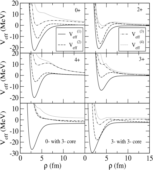
Figure 3: The four lowest adiabatic effective potentials $V^{(n)}_{eff}$ for positive parity states in ¹⁸Ne built on the $0^{+}$ core structure and with total angular momentum $J^{\pi}=0^{+},2^{+},3^{+},4^{+}$ and also $J^{\pi}=0^{-},3^{-}$ for $3^{-}$ core. The proton-core potential is I for the $0^{+}$ core cases and potential IV for the $3^{-}$ core case as given in table 1.

3.1 Effective potentials

The potentials in eq.(3) determine the structure of the ¹⁸Ne states. We show in Fig. 3 the lowest effective potentials for the bound states and resonances selected among the different structures we have investigated, i.e. $J^{\pi}=0^{\pm},1^{\pm},2^{\pm},3^{\pm},4^{+}$ built on both 0⁺ and 3^- core-structures. We see attractive pockets in the two lowest potentials for the positive parity states built on the 0⁺ core. These potentials are strongly influenced by the bound $s$ and $d$-states in the proton-core potentials. At larger distances they asymptotically approach the energies, $-0.6$ Mev or $-0.1$ Mev, of the ¹⁷F bound states. This reflects the large-distance structure of one proton far away from the ¹⁷F nucleus in the corresponding bound states, i.e. ground state, $d_{5/2}$, and first excited state, $s_{1/2}$.

For the total angular momentum, $0^{+}$, the last proton is in either $d$ or $s$-waves around the corresponding ¹⁷F structures. The $2^{+}$ potentials can have ¹⁷F nucleus in the $d_{5/2}$-state surrounded by the second proton with an angular momentum of either $0,2$ or $4$ in total allowing $5$ different couplings. We only include the three lowest of these potentials which approach $-0.6$ MeV. The fourth of the $2^{+}$ potentials in Fig. 3 approaches $-0.1$ MeV. It corresponds to the ¹⁷F nucleus in the $s_{1/2}$-state where the second proton has angular momentum $2$ around ¹⁷F subsystem. At small distances two of these potentials exhibit rather appreciable attraction.

The $4^{+}$ potentials allow proton angular momenta of $2,4,6$, and $4$ around the ¹⁷F nucleus in $d$ or $s$-states, respectively. We find that two of these potentials approach $-0.6$ MeV and one approaches $-0.1$ MeV at large distance. For the $3^{+}$ potentials the angualr momentum combinations are $2,4,6$, or $2,4$, for the bound $d$ and $s$-states, respectively. The lowest potentials again approach $-0.6$ MeV and $-0.1$ MeV. Most of the higher-lying potentials approach zero reflecting a genuine three-body continuum structure.

The lowest effective potentials for negative parity states built on the $0^{+}$ core structure can also be computed with the help of the single-particle $p$-waves. Using $p$-wave interaction from the $s$ and $d$-waves in potential I we find again relatively attractive pockets in the lowest adiabatic potentials for $1^{-}$ and $3^{-}$ but they are almost totally absent for $0^{-}$ and $2^{-}$. The large-distance approaches are found in all cases towards the $s$ and $d$-wave two-body structures. Bound states or resonances of corresponding structures may then arise for $1^{-}$ and $3^{-}$.

The potentials for the $0^{-}$ and $3^{-}$ states built on an excited $3^{-}$ ¹⁶O-core state are also shown in Fig.3. Similar but less attractive potentials are found for 1^- and $2^{-}$. The threshold energy for all these states is then with respect to this core excited state at $6.13$ MeV above the $0^{+}$ ground state of ¹⁶O. The two-body states used to adjust the interactions are bound with respect to this core excited state. These three-body potentials also exhibit attractive pockets at small distances. Their large-distance asymptotics also reflect these two-body “bound states” where the three lowest potentials approach $-3.6$ MeV, $-2.9$ MeV and $-2.1$ MeV. These values correspond to the proton-core “bound” states of $(\ell,S)=(2,5/2),(0,5/2),(2,7/2)$ where $\ell$ is the orbital angular momentum and $S$ the total spin quantum number including the $3^{-}$ from the core.

At small distances several attractive pockets appear. For $0^{-}$ only one deep and broad potential can bind with respect to the $3^{-}$ excited core state. This is essentially due to an even combination of the $(\ell,S)=(2,5/2),(0,5/2)$ partial waves. For $1^{-}$, $2^{-}$ and $3^{-}$ two attractive potentials are found with varying relative depths. They are mostly constructed from those combinations of $(\ell,S)=(2,5/2),(0,5/2),(2,7/2)$ which allow spatially overlapping antisymmetric two-proton states.

3.2 Three-body energies

For each set of adiabatic potentials we solve the coupled set of radial equations in eq.(3). The resulting eigenvalues are shown in tables 3 and 4 for bound and unbound solutions, respectively. If the energies are decisive for applications, as for breakup and decaying resonances, we can fine tune by use of the effective three-body potentials, $V_{3b}(\rho)$, in eq.(3). This would maintain the structure essentially completely unchanged. Such adjustments are not included in the eigenvalue tables.

Table 3: Spectrum of the positive parity bound states in ¹⁸Ne for the different proton-core interactions in table 1. The numerical results have been obtained without inclusion of a three-body potential in Eq.(3). The two-proton separation energies are given in MeV. The last column gives the available experimental energies from til95 .

	$W_{I}$	$W_{II}$	$W_{III}$	$E_{exp}$
$0^{+}_{1}$	$-4.30$	$-5.06$	$-5.32$	$-4.52$
$2^{+}_{1}$	$-2.81$	$-3.19$	$-3.32$	$-2.63$
$4^{+}$	$-1.24$	$-1.17$	$-1.14$	$-1.14$
$0^{+}_{2}$	$-0.46$	$-0.49$	$-1.38$	$-0.94$
$2^{+}_{2}$	$-0.89$	$-0.91$	$-0.88$	$-0.90$
$3^{+}$	$-0.08$	$-0.11$	$-0.02$	$+0.04$

The unbound states are decaying resonances with a width arising from cluster, or equivalently two-proton, emission. To compute such continuum states complex scaling could be applied. States built on the excited $3^{-}$ core state with energies less than 6.13 MeV are bound states in the computation and complex scaling is not needed. They can only decay electromagnetically, or by the neglected coupling to the $0^{+}$ ground state. In any case we focus in this paper only on the real part of the energies which above their respective thresholds are computed in two steps. First a sufficiently attractive three-body potential is added to bind the state. Second the strength of that potential is varied and the resulting energy is extrapolated to the estimated energy obtained for zero strength. This is the so called analytic continuation of the coupling constant method tan97 , which is especially relevant for states arising from the potentials for negative parity states based on the $0^{+}$ core.

The bound states shown in table 3 for different potentials are quite stable independent of choice of potential. In all cases the level ordering is reproduced and the energies are also rather close to the measured values. We only adjusted the potentials to two-body bound state and resonance properties with the simplest possible radial shapes. Potential I leads in general to less binding but closer to measurements than the two other potentials. The deviations are less than $200$ keV except for the $500$ keV underbinding of the last $0^{+}$ state.

In potential I the phase equivalent $s$-wave potential produces a repulsive core at short distance and the valence protons are pushed away from the center. This implies that potential III should bind more when proton-core $s$-wave configurations are substantial as for the first $2^{+}$, the $3^{+}$, and both the $0^{+}$ states. The energies of both the second $2^{+}$ and the $4^{+}$ states do not depend on the chosen potential but matches almost perfectly the measured values. The $3^{+}$ state is weakly bound by less than about $100$ keV in the computation in agreement with the measured value close to the breakup threshold.

The results from potential I and II deviate surprisingly much for the two lowest states indicating that the $p$-wave components play a role. Then the description from potential II implies that these states have contributions of proton-core single-particle $p_{1/2}$ character. This is inconsistent with the shell structure of the core-nucleus. We prefer potentials I and III with the much weaker $p$-wave attraction. Potential I fits the experimental values better than potential II.

As shown in table 4 we find a $3^{-}_{2}$ resonance at about $3.10$ MeV and a low-lying $1^{-}_{1}$ resonance at about $0.2-0.4$ MeV. Both states are based on the $0^{+}$ core ground state. These values are more uncertain since they are obtained by extrapolation with a strongly attractive three-body potential. These structures are not present for $0^{-}$ and $2^{-}$ as already seen from the disappearance of attractive pockets in the lowest adiabatic potentials for negative parity states based on the $0^{+}$ core.

An alternative to potential II in descriptions of the negative parity states is potential IV. We show several of the resulting energies in table 4. In particular there appears a $1^{-}_{2}$ state built on the excited $3^{-}$ core state and bound compared to this state by $3.98$ MeV implying that it is an observable resonance at about $2.12$ MeV. Since the energies of the two $1^{-}$ states differ by $2$ MeV they may be decoupled in practice. The $0^{-}$ energy is about $-5.45$ MeV with respect to the core excited state and therefore at an energy of $0.58$ MeV above the two-proton threshold.

We find another $3^{-}$ “bound” state at about $-3.09$ MeV corresponding to $1.33$ MeV. For $2^{-}$ we find two “bound states at about $-2.92$ MeV and $-2.00$ MeV corresponding to $3.41$ MeV and $4.13$ MeV. The second of these is a resonance in the two-body continuum of the bound proton-¹⁶O($3^{-}$) system and the other proton. There is no confining barrier and it easily leaks out corresponding to a large width. All these negative parity states can easily be matched to measured energies in the continuum. However, such a comparison is not very revealing due to the inevitable inaccuracy from the three-body approximations. At least more structure information is needed. Still we show some of the lowest measured values in table 4. Many higher-lying levels are found experimentally.

Table 4: Spectrum of the unbound, mostly negative parity, states in ¹⁸Ne for different proton-core interactions in table 1. The numerical results have been obtained without inclusion of a three-body potential in Eq.(3). The two-proton separation energies are given in MeV with respect to the threshold for separation into two protons and the core in its ground state. These energies are given below the potentials used in the computation. The fifth and sixth columns give the available experimental energies and spin and parities, if known, from til95 . The computations with potential IV are for a core-excited state at 6.13 MeV implying that these states with energies lower than 6.13 MeV behave as bound states.

$J^{\pi}$	$W_{I}$	$W_{III}$	$W_{IV}$	$E_{exp}$	$J^{\pi}_{exp}$
$1^{-}_{1}$	$0.44$	$0.20$		$0.00$	$1^{-}$
$0^{-}$			$0.58$	$0.57$	$(2^{+},3^{-})$
				$0.63$	$(2^{+},3^{-})$
$3^{-}_{1}$			$1.33$	$0.93$
$1^{-}_{2}$			$2.12$	$1.63$	$1^{-}$
$3^{-}_{2}$	3.10	3.10
$2^{-}_{1}$			$3.41$
$2^{-}_{2}$			$4.13$

3.3 Wavefunctions

The eigenfunctions are found as expansion coefficients on the hyperharmonic basis with quantum numbers for each of the Faddeev components, i.e. ($\ell_{x},\ell_{y},L,s_{x},S,J$). Each eigenfunction can be expressed in one set of Jacobi coordinates with corresponding probabilities depending on potential and quantum numbers. We shall in this section in details discuss the two bound 0⁺ states and the 1^- resonance located close to the threshold. For completeness we give the decompositions of the other states in the appendix.

Table 5: Components included in the calculations for the 0⁺ states. The upper part correspond to the first Jacobi set ($x$ between the two protons). The lower part corresponds to the second and third Jacobi sets ($x$ from core to proton). The 6^th column gives the maximum value of the hypermomentum used for each component. The last three columns give the contribution from each component to the 0⁺ wave functions for potentials I, II and III respectively. Only contributions larger than 0.1 is given. The two numbers for each component correspond to the $0^{+}_{1}$ and $0^{+}_{2}$ states, respectively.

$\ell_{x}$	$\ell_{y}$	$L$	$s_{x}$	$S$	$K_{max}$	$W_{I}$	$W_{II}$	$W_{III}$
0	0	0	0	0	120	80.7	81.0	78.9
						82.0	82.2	86.6
1	1	1	1	1	90	17.0	17.0	17.1
						8.9	8.5	9.7
2	2	0	0	0	90	2.3	2.1	3.9
						9.1	9.3	3.7
0	0	0	1/2	0	120	24.9	21.9	44.4
						74.3	76.0	53.1
1	1	0	1/2	0	90	5.0	13.2	0.4
						0.4	0.3	4.3
1	1	1	1/2	1	85	0.2	1.5	0.2
						0.2	0.3	0.1
2	2	0	1/2	0	100	52.6	47.5	37.4
						16.1	14.9	32.6
2	2	1	1/2	1	90	17.3	15.9	17.6
						9.1	8.5	9.8

3.3.1 Bound states

The available single-particle states for the two protons are $d_{5/2}$ and $s_{1/2}$ orbits. Two-particle states of both protons in $d_{5/2}$ produce the sequence of $0^{+}$, $2^{+}$, and $4^{+}$ states where the odd angular momenta are forbidden due to the antisymmetry requirement. Using two $s_{1/2}$ states we can only produce a $0^{+}$ state. One proton in each of the $d_{5/2}$ and $s_{1/2}$ states produce one $2^{+}$ and one $3^{+}$ state. As seen in Fig. 1 they all appear in the computed spectrum. The partial wave decomposition reveal the microscopic structure of the states.

We show the partial wave decomposition in table 5 for the two $0^{+}$ states. The upper part using the first Jacobi system, where the $x$-coordinate connects the two protons, exhibits only small variation between results from the different potentials, the $s$-waves of about $80$% dominate for both states in the three cases.

The picture is very different in the proton-core Jacobi system where the variation with potential is larger. The $0^{+}_{2}$ state with potential I has about $74\%$ in the $s_{1/2}^{2}$ configuration which essentially means that both protons are in $s_{1/2}$-states. With potential III the components $d_{5/2}$ and $s_{1/2}$ are more even, i.e. about $55\%$ $d_{5/2}^{2}$ in $0^{+}_{1}$ and $53\%$ $s_{1/2}^{2}$ in $0^{+}_{2}$. This reflects the lack of repulsion at short distance in the $s$-wave interaction which favor $s$-waves in the ground state. With potential II we still get about $76\%$ $s_{1/2}^{2}$ configuration in the $0^{+}_{2}$ state. We also included components with $\ell_{x}$ and $\ell_{y}$ larger than 2 although their contributions are found to be negligible after the computations as we already mentioned in section 2.3.

The configurations obtained here for the $0^{+}_{2}$ state essentially only contains $sd$-waves. Early shell model calculations of both mirror nucleus ¹⁸O law74 and ¹⁸Ne she98 gave about $33\%$ and collective motion the remaining $67\%$. Our computed energy only deviates from measurements by about $0.4$ MeV, see table 3, which is a typical deviation in such three-body calculations. This is therefore surprising if $2/3$ of the structure should have a completely different origin. It is more likely that the $sd$-configurations contribute by more than $1/3$ to the $0^{+}_{2}$ structure. This may be reconciled with the shell model results if part of the collective motion also is of $sd$-character.

The other four bound states of $J^{\pi}=2^{+},3^{+},4^{+}$ are also decomposed in partial wave configurations and shown as tables in the appendix. Both $2^{+}$ and $3^{+}$ states consist of proton-core $s$ and $d$-waves, and the $4^{+}$ state of solely $d$-waves.

3.3.2 Unbound states

With potential II it is a priori not excluded to find negative parity energies with resemblance to the measured spectrum. The corresponding structures are on the other hand not expected to reproduce measured properties. The basic problem is the assumption of a single-particle $p_{1/2}$-state in the low-lying spectrum of ¹⁷F. Potential IV, built on the core excited $3^{-}$ state is in general expected to provide better structure properties. Then a number of $0^{-},1^{-},2^{-},$ and $3^{-}$ states should arise as combinations of $d$ and $s$ states coupled to the $3^{-}$ core state. However, it is here worth emphasizing that there might be different, perhaps essentially uncoupled, structures of the same $J^{\pi}$ but built on different core states. We find such states with $J^{\pi}=1^{-}$ and $3^{-}$.

Table 6: The same as table 5 for the 1${}^{-}_{1}$ state in ¹⁸Ne with the 0⁺ core.

$\ell_{x}$	$\ell_{y}$	$L$	$s_{x}$	$S$	$K_{max}$	$W_{I}$	$W_{III}$
0	1	1	0	0	120	82.9	80.4
1	0	1	1	1	80	6.0	8.1
2	1	1	0	0	80	5.3	5.7
1	2	1	1	1	80	3.5	2.7
1	2	2	1	1	80	2.3	3.1
0	1	1	1/2	0	100	19.4	19.6
0	1	1	1/2	1	80	1.4	1.6
1	0	1	1/2	0	100	19.1	21.2
1	0	1	1/2	1	80	0.9	1.1
2	1	1	1/2	0	100	29.7	22.4
2	1	1	1/2	1	80	5.0	4.7
2	1	2	1/2	1	80	1.9	2.1
1	2	1	1/2	0	100	21.8	21.0
1	2	1	1/2	1	80	4.3	4.4
1	2	2	1/2	1	80	1.7	1.9

The first $1^{-}_{1}$ state is built on the $0^{+}$ core ground state. The cluster model ¹⁴O+$\alpha$ in duf04 cannot describe this state which is suggested as a candidate for burning ¹⁸Ne into water while releasing a lot of energy bel01 . The decomposition shown in table 6 is in the first Jacobi system seen to be dominated by $s$-wave components between the two protons. In the other Jacobi system both proton-core $s$ and $d$-waves contribute about $20\%$ and $p$-waves by twice that amount. In this way the attraction of the two interactions, $s_{1/2}$ and $d_{5/2}$, are optimized. The lowest adiabatic potential contributes by $93\%$.

Table 7: The same as table 5 for the second 1${}^{-}_{2}$ state in ¹⁸Ne with the 3^- core excited state.

$\ell_{x}$	$\ell_{y}$	$L$	$s_{x}$	$S$	$K_{max}$	$W_{IV}$
2	0	2	0	3	60	1.7
0	2	2	0	3	60	3.3
1	1	2	1	2	100	89.4
1	1	2	1	3	60	4.3
2	2	2	0	3	60	1.3
0	2	2	5/2	2	100	44.6
0	2	2	5/2	3	100	0.2
2	0	2	5/2	2	100	45.2
2	0	2	5/2	3	100	9.4
1	1	2	5/2	2	100	0.6

The second $1^{-}_{2}$ state is built on the $3^{-}$ excited core state. The three-body decay of this state into two protons and the ground state of ¹⁶O is measured and analysed in terms of sequential, virtual sequential and direct decay branching ratios ras08 ; gom01 . Such decay must take place through couplings to other states as this state is bound with respect to the $3^{-}$ core excited state. The decomposition in table 7 show dominance of $p$-waves in the first Jacobi system. In the other Jacobi systems this results in equal amounts of $s$ and $d$-waves in the proton-core subsystem. This implies that the proton-core spin has to be $5/2$. The lowest and second potential contribute by $88\%$ and $11\%$, respectively.

We find several differences with respect to the shell model results in bro02 where the structure of the different $1^{-}$ states in ¹⁸Ne are discussed in detail. The first five of these shell model $1^{-}$ states have for one choice of interactions respectively about $2\%$, $20\%$, $6\%$, $12\%$, $49\%$ of configurations with ¹⁶O in the ground state. For comparison our two $1^{-}$ states contain $100\%$ either ground or $3^{-}$ excited state of ¹⁶O. The shell model results strongly indicate mixing of different excited states of ¹⁶O coupled to the two protons. However, these shell model structures at most determine the short-distance behavior whereas the intermediate and large-distance structures can be completely different and hence also the resulting momentum distributions after decay.

The partial wave decomposition of all other computed unbound states are shown in the appendix. The $0^{-}$ and the two $2^{-}$ built on the core excited $3^{-}$ state all consist of proton-core $s$ and $d$-waves. The two $3^{-}$ states consist of proton-core $p$-waves and $p$ and $d$-waves when built on the $3^{-}$ and $0^{+}$ core states, respectively.

The partial wave decomposition focus on the angular structure. The structures can be further characterized by the overlaps between valence wavefunctions of negative and positive parity states. Here it is necessary to remember that the core structure differs, and true overlaps are zero. However, the valence part may have contributions of precisely the same partial waves which in turn has to be coupled to $0^{+}$ or $3^{-}$ to give the different total angular momenta. The overlaps can be estimated from the partial wave decompositions in the tables. These angular overlaps should be multiplied by radial overlap functions which in general are rather similar for low-lying states. The orbital and spin angular momentum couplings introduce in some cases another substantial reduction factor. It is in this way easily seen that the two $0^{+}$ states and the $3^{-}$ state have the largest overlaps both exceeding $0.6$. Also the $3^{+}$ and the $0^{-}$ states seem to overlap by more than $0.4$ similar to the first $2^{+}$ and the first $2^{-}$ states. All other overlaps are rather small.

4 Moments and transition probabilities

The expectation values of the operators provide observables for each state. The most interesting are those related to sizes and lifetimes. We give details in the next two subsections.

4.1 Relative sizes

The sizes are observable quantities, where the simplest are the second moments of charge and matter distributions. These are the root mean square radii which often only are available for the ground state. The charge radius is most accurately obtained by electromagnetic probes like electrons. The matter radius is for light nuclei derived from measurements of interaction cross sections. The excited states are closer to the threshold for breakup and therefore more likely to develop a spatially extended halo structure. This would have observable implications for breakup cross sections. Effects of binding energy and angular momentum are both important jen04 . The three-body results are related to observables by including the finite extension of core distribution for matter and charge. In the present case we have for the matter distribution

$$\langle r^{2}\rangle = \frac{16}{18}r^{2}_{core}+\frac{1}{18}\langle\rho^{2}\rangle\;,$$ (7)

$$\langle\rho^{2}\rangle = \frac{1}{2}\langle r^{2}_{pp}\rangle+\frac{32}{18}\langle r^{2}_{c,pp}\rangle=\frac{16}{17}\langle r^{2}_{pc}\rangle+\frac{17}{18}\langle r^{2}_{p,cp}\rangle\;,$$

where $r^{2}_{core}$ is the mean-square radius of the core. For the charge distribution we get

$$\langle r^{2}\rangle_{ch} = \frac{8}{10}r^{2}_{core,ch}+\frac{1}{20}\langle r^{2}_{pp}\rangle+\frac{136}{810}\langle r^{2}_{c,pp}\rangle\;,$$ (8)

$$\frac{\langle r^{2}\rangle_{ch}}{\langle r^{2}\rangle} = \frac{9}{10}\frac{r^{2}_{core,ch}+\langle r^{2}_{pp}\rangle/16+17\langle r^{2}_{c,pp}\rangle_{ch}/81}{r^{2}_{core}+\langle r^{2}_{pp}\rangle/32+\langle r^{2}_{c,pp}\rangle_{ch}/9}\;,\;$$ (9)

where $r^{2}_{core,ch}$ is the mean-square radius of the core charge distributions. We assume that charge and matter distributions are identical for the core. With these expressions we can always insert a different value for the core moments if better parameters become available.

4.1.1 Bound states

The root-mean-square, charge and matter, radii for the computed bound states are given in table 8. The results are essentially independent of the core-proton potential but the trends reflect that smaller binding energies give larger radii and viceversa. This is especially clearly seen for the $0^{+}_{2}$ state where potential III gives more binding and smaller radius. Comparing the different $0^{+}$ and $2^{+}$ states the tendency is also clearly that the smallest binding lead to the largest radius. The trends for angular momentum is that $s$-waves easier extend to larger distances whereas $d$-waves and higher are confined by the centrifugal barrier. This is seen for the $3^{+}$ state which is weaker bound with smaller angular momenta than the $4^{+}$ state, and consequently also significantly larger.

When we assume equal matter and charge radius for the core we find that the charge radii are slightly larger than the corresponding matter radii. This is in spite of the “natural” reduction factor of $9/10$ in Eq.(9). The reason is found in a core radius which is substantially smaller than both the proton-proton distance as well as the distance from their center of mass and the core, see table 9. Combined with a smaller weight in Eq.(9) on these terms for matter compared to charge radii this results in these larger charge radii. Recent measurements confirm that the charge radius is larger than the matter radius gei08 ; oza01 . If we compare our values with FMD calculations gei08 we can see that our matter radius is bigger and closer to experimental data. On the other hand the FMD charge radius is in better agreement with the experimental value.

Table 8: Root mean square (rms) radii in fm for the different bound states in ¹⁸Ne with the three proton-core interactions. Charge and matter radii are shown in first and second row, respectively. They employ the root-mean square radius of $2.71$ fm for the ¹⁶O core. The only known experimental values for ¹⁸Ne are the root mean square charge radius, 2.971$\pm$0.020 fm gei08 , and matter radius, 2.81$\pm$0.14 fm oza01 , for the ground state. In gei08 we can also find FMD calculations that give 2.93 fm and 2.70 fm for the charge and matter radii of the ground state.

	$W_{I}$	$W_{II}$	$W_{III}$
$0^{+}_{1}$	$2.82$	$2.80$	$2.74$
	$2.78$	$2.77$	$2.73$
$2^{+}_{1}$	$2.86$	$2.84$	$2.78$
	$2.80$	$2.79$	$2.75$
$4^{+}$	$2.82$	$2.83$	$2.84$
	$2.78$	$2.78$	$2.79$
$0^{+}_{2}$	$3.08$	$3.30$	$2.80$
	$2.93$	$3.07$	$2.76$
$2^{+}_{2}$	$2.92$	$2.92$	$2.86$
	$2.84$	$2.83$	$2.80$
$3^{+}$	$3.47$	$3.44$	$3.30$
	$3.17$	$3.15$	$3.06$

The average size can be distributed between distances of the different constituents, i.e. in the present case the proton-core and proton-proton distances. These root mean square radii for the computed bound states are given in table 9 for the different potentials. These two-body distances within the three-body system also follow the general trends of binding energy and angular momentum. The distance between the two protons is in all cases larger than the proton-core distance. This is because the proton-core attraction is decisive for the binding of all three-body states. For the weakly bound $3^{+}$ state this difference is substantially larger due to the small binding energy. The sizes show that the protons are located substantially outside the surface of the core. This is obviously helping to decouple core and valence degrees of freedom, and validate the model assumptions in the treatment as a three-body system. In general the trends from the overall rms radii in table 8 are maintained.

Table 9: For the different computed states in ¹⁸Ne, and the different proton-core potentials, root mean square distances (in fm) $\langle r_{pp}\rangle^{1/2}$ and $\langle r_{cp}\rangle^{1/2}$, where $p$ and $c$ denote an external proton and the core, respectively.

		$W_{I}$	$W_{II}$	$W_{III}$
$0^{+}_{1}$	$\langle r^{2}_{pp}\rangle^{1/2}$	4.0	3.7	3.4
	$\langle r^{2}_{cp}\rangle^{1/2}$	3.4	3.3	3.0
$2^{+}_{1}$	$\langle r^{2}_{pp}\rangle^{1/2}$	4.3	4.0	4.0
	$\langle r^{2}_{cp}\rangle^{1/2}$	3.5	3.5	3.2
$4^{+}$	$\langle r^{2}_{pp}\rangle^{1/2}$	4.3	4.4	4.4
	$\langle r^{2}_{cp}\rangle^{1/2}$	3.4	3.4	3.5
$0^{+}_{2}$	$\langle r^{2}_{pp}\rangle^{1/2}$	6.0	6.6	4.5
	$\langle r^{2}_{cp}\rangle^{1/2}$	4.4	5.2	3.2
$2^{+}_{2}$	$\langle r^{2}_{pp}\rangle^{1/2}$	4.8	4.8	4.8
	$\langle r^{2}_{cp}\rangle^{1/2}$	3.8	3.8	3.5
$3^{+}$	$\langle r^{2}_{pp}\rangle^{1/2}$	8.2	8.1	7.5
	$\langle r^{2}_{cp}\rangle^{1/2}$	5.8	5.7	5.2

The average sizes in tables 8 and 9 are results of the probability distributions. They are shown in Fig.4 for the two $0^{+}$ states as functions of the distances between the two protons and their center-of-mass and the core. Both distributions have a tail in the proton-proton distance extending to about $10$ fm. The fall-off in $r_{c,pp}$ seems to be faster reaching no more than about $5$ fm. The ground state has two separated peaks around the points $(r_{pp},r_{c,pp})\approx$ $(1.5,2.7),$ $(5.0,0.8)$ (all in fm) where the last is much smaller and somewhat broader. In contrast the second $0^{+}$ state has only one peak at $(r_{pp},r_{c,pp})\approx(4.2,2.2)$. Since the angular momentum decompositions are rather similar these differences must arise from the interference between the adiabatic components. The prominent peak in $0^{+}_{1}$ is in $0^{+}_{2}$ moved to larger distances between the protons and the small peak is at the same time moved to somewhat larger distances in $r_{c,pp}$. The result is that $0^{+}_{2}$ has one broad peak.

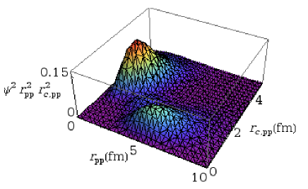
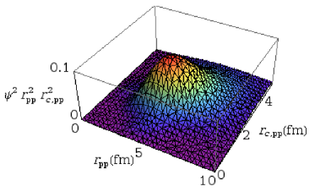
Figure 4: Contour diagram for the probability distribution of 0${}^{+}_{1}$ (upper) and 0${}^{+}_{2}$ (lower) states in ¹⁸Ne. The square of the three-body wave function is integrated over the directions of the two Jacobi coordinates.

The same pattern is found for the two $2^{+}$-states with two peaks for $2^{+}_{1}$ at $(r_{pp},r_{c,pp})\approx(1.9,2.7),(5.0,1.0)$ and one broad peak for $2^{+}_{2}$ at $(r_{pp},r_{c,pp})\approx(5.0,1.8)$. The positions are also almost the same as for the $0^{+}$-states where the latter position tends to be at smaller distances. The $4^{+}$-state has one peak at $(r_{pp},r_{c,pp})\approx(3.5,2.0)$ which is an almost equal sided triangle. The $3^{+}$-state has one peak at $(r_{pp},r_{c,pp})\approx(4.6,2.2)$.

4.1.2 Unbound states

The negative parity states are in principle all resonances but except for the $1^{-}_{1}$ $3^{-}_{2}$ states they are all computed as bound states with respect to the $3^{-}$ core excitation. Therefore the radial moments are for these ($3^{-}$ based) well defined and together with partial wave decomposition characteristic for the structures. In table 10 we give root mean square radii of matter and charge together with distances between protons and core for these states. Here in order to calculate matter and charge radii we have used the same radii for the core.

Table 10: Root mean square (rms) radii in fm for different negative parity resonances in ¹⁸Ne with proton-core interactions III (for the $1^{-}_{1}$ state) or IV (for the $1^{-}_{2}$, $0^{-}$, $3^{-}_{1}$, and $2^{-}$ states). Charge and matter radii are shown in second and third column. We used the root-mean square radius, $2.71$ fm, of the ¹⁶O ground state instead of the unknown value for the $3^{-}$ excitation. In the fourth and fifth column we show root mean square distances (in fm) $\langle r_{pp}\rangle^{1/2}$ and $\langle r_{cp}\rangle^{1/2}$, where $p$ and $c$ denote an external proton and the core, respectively.

	$\langle r_{c}^{2}\rangle^{1/2}$	$\langle r^{2}\rangle^{1/2}$	$\langle r_{pp}\rangle^{1/2}$	$\langle r_{cp}\rangle^{1/2}$
$1^{-}_{1}$	$3.00$	$2.88$	$5.80$	$4.12$
$1^{-}_{2}$	$2.86$	$2.80$	$4.36$	$3.26$
$0^{-}$	$2.77$	$2.75$	$4.11$	$3.10$
$3^{-}_{1}$	$2.72$	$2.72$	$3.64$	$2.88$
$2^{-}_{1}$	$3.01$	$2.90$	$4.37$	$3.87$

As for the positive parity bound states the charge radii are usually slightly larger than matter radii, see table 10. In general the positive and negative parity states are almost of the same size even though the binding to the $3^{-}$ core is larger by several MeV. Also the internal distances remain essentially the same with the proton distance as the largest. Not surprisingly the tendencies with binding energy and angular momentum follow the general rules explained for the positive parity states. Only the $1^{-}_{1}$ state of roughly zero energy has a sufficiently well defined radial structure to be included in table 10.

The probability distributions are all rather similar. Both $1^{-}$-states have only one well-defined peak at $(r_{pp},r_{c,pp})$ $\approx(1.9,2.7),(3.5,1.8)$. The first of these resemble the lowest $0^{+}$ and $2^{+}$state and the second more resembles the $4^{+}$ state. We also find one peak for both $0^{-}$, $2^{-}_{1}$ and $3^{-}_{1}$-states at $(r_{pp},r_{c,pp})\approx$ $(3.1,1.6),(1.9,2.2),$ $(2.3,1.6)$. For $2^{-}_{1}$ a second peak is indicated at the side of the main peak resulting in an intermediate structure between the two we have already seen for bound states (see Fig. 5). The $0^{-}$ state resemble the $4^{+}$ state with the two protons close to the core but rather far from each other.

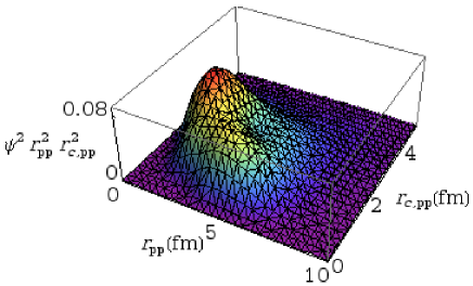
Figure 5: Contour diagram for the probability distribution of 2${}^{-}_{1}$ state in ¹⁸Ne. The square of the three-body wave function is integrated over the directions of the two Jacobi coordinates.

The probability distributions for the resonances built on the $0^{+}$ core ground state are not well defined since their energies are above threshold and the radial wavefunctions therefore spread out to infinitely large distances. However, they all have large amplitudes around the minimum in the corresponding adiabatic potentials.

4.2 Electromagnetic decays

The bound states can only decay electromagnetically. The corresponding observable transition probabilities are critically depending on the structures. Thus they provide experimental tests and we therefore compute the lifetimes for future comparison. The three-body states below $6.13$ MeV built on the core-excited $3^{-}$ state are also bound states. They can therefore only decay by $\gamma$-emission to lower lying states either by maintaining the same cluster structure or by $E3$-decay of the core excited state. In both cases we can compute the electromagnetic transition probabilities. The selection rules determine the dominating transitions which can be of both electric and magnetic origin.

The effective charge of the proton $e_{eff}$ is for these estimates determined by renormalizing the calculated $E2$-transition strength from first excited to ground state in ¹⁷F to the measured value of 25 Weisskopf units or $62.96$e² fm⁴ til95 . This gives a value amazingly close to unity $e_{eff}/|e|=0.99$ which is used in the three-body computations.

The structures are sufficiently similar for the different interactions to allow estimates with only one potential for each state. We choose potential I and IV for positive and negative parity states, respectively. The selection rules determine the dominating transitions which can be of both electric and magnetic origin. Transitions within the same parity are then dominated by $E2$ or $M1$ emissions, and between different parity states predominantly by $E1$. If $E1$ is forbidden the much weaker $M2$ or $E3$ transitions may determine the lifetime, but to this level of accuracy the neglected mixture of ground and excited core-states could contribute.

4.2.1 Multipole operators

The electric multiple operators are defined as:

$${\cal M}_{\mu}(E\lambda)=e\sum_{i=1}^{A}Z_{i}r_{i}^{\lambda}Y_{\lambda,\mu}(\hat{r}_{i})$$ (10)

where $A$ is the number of constituents in the system, each of them with charge $eZ_{i}$, and where $\mbox{\boldmath$r$}_{i}$ is the coordinate of each of them relative to the $A$-body center of mass.

The electric multipole strength functions are defined as:

$${\cal B}(E\lambda,I_{i}\rightarrow I_{f}) = \sum_{\mu M_{f}}|\langle I_{f}M_{f}|{\cal M}_{\mu}(E\lambda)|I_{i}M_{i}\rangle|^{2}$$ (11)

$$= \frac{1}{2I_{i}+1}|\langle I_{f}||{\cal M}(E\lambda)||I_{i}\rangle|^{2}$$

The ${\cal M}_{\mu}(E\lambda)$ operator in Eq.(10) can then be rewritten as:

$${\cal M}_{\mu}(E\lambda) = e\sum_{i=1}^{A-2}Z_{i}|\mbox{\boldmath$r$}_{c}+\mbox{\boldmath$r$}_{i}^{\prime}|^{\lambda}Y_{\lambda,\mu}(\widehat{\mbox{\boldmath$r$}_{c}+\mbox{\boldmath$r$}_{i}^{\prime}})$$ (12)

$$+ e\sum_{j=1}^{2}Z_{j}r_{j}^{\lambda}Y_{\lambda,\mu}(\hat{r}_{j})$$

where the index $i$ runs over the $A-2$ constituents in the core, and $j$ labels the two external nucleons.

As in rom08 we can rewrite into intrinsic core and external valence nucleon coordinates. The results turn out to have the form

$${\cal M}_{\mu}(E\lambda)=e\sum_{i=1}^{3}Z_{i}r^{\lambda}_{i}Y_{\lambda,\mu}(\hat{r}_{i})+{\cal M}_{\mu}(E\lambda,c)$$

$$+ \sum_{k=1}^{\lambda-1}\sum_{m=-k}^{k}f_{\lambda}(k,m,\mu)r_{c}^{k}Y_{k,m}(\hat{r}_{c}){\cal M}_{\mu-m}(E(\lambda-k),c)$$

where the two first terms refer to independent valence and core degrees of freedom, respectively. The last terms describe simultaneous transitions of core and valence particles where $f(m,\mu)$ is a well defined function of its indices. Then, since the only allowed core transition is ${\cal M}_{\mu}(E3)$, only the second term contributes to transitions between the two different core states. For transitions between the same core state the mixed terms may in principle contribute. However, these terms are accounted for by the effective charge of the proton which was adjusted to describe the $E2$-transition in ¹⁷F. Thus also these terms should not be included.

The magnetic multipole operator, ${\cal M}_{\mu}(M\lambda)$, has the opposite parity of ${\cal M}_{\mu}(E\lambda)$ and give rise to much smaller rates for the same $\lambda$. Thus ${\cal M}_{\mu}(M2)$ only is active between negative parity states where the $E3$ core transition is necessary in the present cases. The $(M2)$ transitions are then forbidden. On the other hand $(M1)$ conserves parity, allows unchanged core structure, and may compete with $(E2)$ transitions. We shall therefore only consider the $(M1)$ operator which is defined as:

$${\cal M}_{\mu}(M1)=\frac{e\hbar}{2Mc}\sqrt{\frac{3}{4\pi}}\sum_{i}(g^{(i)}_{s}\vec{s}_{i}+g^{(i)}_{\ell}\vec{\ell}_{i})_{\mu}\;,$$ (14)

where $\mu$ labels the spherical component of an operator, and the constants $g_{s}$ and $g_{\ell}$ depend on the constituent particles $i$. The magnetic multipole transition strength is defined as for the electric case (see Eq.(11)).

The core has a charge of $8$ units suggesting that $g_{\ell}^{(c)}=8$. For the positive parity states where the core angular momentum is zero we use a vanishing effective spin $g$-factor, i.e. $g_{s}^{(c)}=0$. For the negative parity states where the core angular momentum is $3$ the $g$-factor is unknown but also of little interest since the dominating decay probabilities are determined by other transitions. We use the free proton value of $g_{s}^{(p)}$=$5.586$ and we use again an effective proton charge $g_{\ell}^{(p)}$=$0.99$. The relevant transition operators are then defined and we can compute the observable transition strengths.

4.2.2 Transition strengths

The ${\cal B}(E2)$-transition for ¹⁷F from $1/2$ to $5/2$ amounts to about $63$e²fm⁴ corresponding to $25$ W.u. and a width of $1.6\times 10^{-6}$ eV til95 . This is within $1\%$ the same as computed from the relative two-body wavefunctions. This indicates that an effective charge of $1$ should be used for the low-energy sequence of states in ¹⁸Ne which all are dominated by $E2$ transitions. We collect in table 11 the four possible ${\cal B}(E2)$ values from first and second $2^{+}$ to the other positive low-lying parity states. As usual the reduced matrix element should be multiplied by $1/(2J_{i}+1)$ depending on initial and final states in the transition. The table values include this factor and reflect the chosen direction of the transition.

Table 11: $E2$-transition strengths from first and second $2^{+}$ states to neighboring $J^{+}$ states expressed in units of $e^{2}$ fm⁴. The first two rows (upper part) contain measured values from til95 . The next two rows (central part) correspond to our calculation. The last two rows (lower part) show computed values obtained in duf04 .

${\cal B}$	$0_{1}^{+}$	$0_{2}^{+}$	$2_{i}^{+}$	$4^{+}$
${\cal B}(E2,2^{+}_{1}\rightarrow J^{+})$	$48(5)$	$2.7(13)$	$-$	$43(6)$
${\cal B}(E2,2^{+}_{2}\rightarrow J^{+})$	$1.8(9)$	$-$	$-$	$-$
${\cal B}(E2,2^{+}_{1}\rightarrow J^{+})$	$21.53$	$2.199$	$2.445$	$31.71$
${\cal B}(E2,2^{+}_{2}\rightarrow J^{+})$	$0.322$	$7.154$	$2.445$	$1.179$
${\cal B}(E2,2^{+}_{1}\rightarrow J^{+})$	$32.09$	$-$	$-$	$59.26$
${\cal B}(E2,2^{+}_{2}\rightarrow J^{+})$	$0.084$	$-$	$-$	$-$

For potential I the computed table values (central part of table 11) are all systematically smaller than the measured results (upper part of table 11), i.e. smaller by factors of 2.2, 1.22, 1.36, respectively for the known $2^{+}_{1}$ transitions in the third row of table 11. For ${\cal B}(E2,2^{+}_{1}\rightarrow 0_{1}^{+})$ there are newer measurements resulting in $23\pm 4e^{2}fm^{4}$ and $27\pm 4e^{2}fm^{4}$ in ril00 which are in better agreement with our values. However, later on the same author published in ril03 the results of a measurement of the life time of this excited $2^{+}_{1}$ state which is more consistent with the value we used from til95 . The computed $2^{+}_{2}\rightarrow 0_{1}^{+}$ transition is smaller by a factor 5.5 but on top of the varying experimental results the measured value in til95 is given with a rather large uncertainty which could reduce this discrepancy to a factor of 2.7. The discrepancies are reduced if we correct all numbers by scaling the root mean square value of the ground state from the calculated $2.78$ fm to the measured value of $2.81$ fm as found in oza01 .

The remaining deviations are now within acceptable ranges for a model where core polarization is neglected. The largest discrepancy appears for the $0^{+}$ state which might have the strongest influence from the lowest core excitation of the same quantum number, $0^{+}$. The phenomenological procedure to correct for that effect is to use an effective charge larger than unity which then accounts for influence beyond the single-particle degrees of freedom. Most of the transitions are substantially larger than corresponding to one single particle unit. This usually is a signal of the need for an effective charge larger than unity which in turn implies that core degrees of freedom are important. On the other hand the transition probabilities are not consistent with collective vibrational motion as the spectrum of excited states otherwise could indicate. Furthermore, the main variation is picked up by the three-body model.

With the radius of $1.2A^{1/3}$ fm the single particle Weisskopf unit for ${\cal B}(E2)$ is 2.690$e^{2}$fm⁴ which indicates that the proton-core $E2$-transition of about $25$ W.u. is constructed by substantially more than a simple single-particle transition. On the other hand this $E2$ transition in ¹⁷F is reproduced with the proper wavefunctions and an effective proton charge of one. Then it is not unreasonable to expect that the three-body system should be approximately describable without active core degrees of freedom as well or perhaps rather with appropriate effective charges from the two-body subsystem.

The transition probability from $2_{2}^{+}$ to $2_{1}^{+}$ receives also a contribution from $M1$. We find ${\cal B}(M1,2^{+}_{2}\rightarrow 2_{1}^{+})=9.7\times 10^{-4}$ $e^{2}$fm² which is smaller than the measured value of $0.0017\pm 0.0007$ $e^{2}$fm² (0.088$\pm$0.038 W.u.) corresponding to a width of $9.5\times 10^{-3}$ eV til95 . The small computed value has the inherent uncertainty arising from spin polarization which can lead to a substantial correction. In any case this decay seems to be dominated by $M1$.

Table 12: $E2$ and $M1$-transition strengths from the second $3^{+}$ state to lower-lying $J^{+}$ states expressed in units of $e^{2}$ fm⁴ and $e^{2}fm^{2}$, respectively. The third row gives the ratio of partial widths for the two decay modes. The fourth and fifth rows shows the values from duf04

${\cal B}$	$2_{1}^{+}$	$4^{+}$	$2_{2}^{+}$
${\cal B}(E2,3^{+}\rightarrow J^{+})$	$0.0596$	$24.0$	$4.27$
${\cal B}(M1,3^{+}\rightarrow J^{+})$	$0.0240$	$1.76\times 10^{-7}$	$1.16\times 10^{-3}$
$\Gamma_{E2}/\Gamma_{M1}$	$1.35\times 10^{-5}$	147	0.00250
${\cal B}(E2,3^{+}\rightarrow J^{+})$	$0.107$	$5.89$	$14.4$
${\cal B}(M1,3^{+}\rightarrow J^{+})$	$1.54\times 10^{-3}$	$3.84\times 10^{-3}$	$1.35\times 10^{-4}$

The decay modes of lowest multipolarity for the $3^{+}$ state are $E2$ and $M1$ where the final state can be any of the three states shown in table 12. The corresponding decay widths are given by $\Gamma_{E2}=4\pi/75(E_{\gamma}/\hbar c)^{5}{\cal B}(E2)$ and $\Gamma_{M1}=16\pi/9(E_{\gamma}/\hbar c)^{3}{\cal B}(M1)$. The ratio of widths is then $\Gamma_{E2}/\Gamma_{M1}=0.03(E_{\gamma}/\hbar c)^{2}{\cal B}(E2)/{\cal B}(M1)$.

The $E2$ transition from $3^{+}$ is dominated by decay to the $4^{+}$ state. The $E2$ transitions to the two $2^{+}$ states are smaller by factors of about $6$ and 30, respectively. These decay probabilities are essentially completely arising from single-particle proton transitions between orbits around the ¹⁷F structure. The relative sizes correspond directly to the probabilities of the largest $E2$ allowed configurations in tables 13, 14 and 15.

The $M1$ transitions are also essentially due to proton transitions between orbits around the ¹⁷F structure. They are all very small but still varying by orders of magnitude. The sizes strongly indicate that the dominating parts of these transitions are forbidden by $M1$ selection rules due to the single particle character of the operator. The decisive selection rules are $\Delta\ell_{x}=\Delta\ell_{y}=0$, and $\Delta s_{x}=\Delta s_{y}=0$. For the $\ell$-part also $\Delta S=0$ and analogously $\Delta L=0$ for the $s$-part. The $3^{+}$ state is from table 15 seen to be dominated by $(\ell_{x},\ell_{y},L,s_{x},S)=(2,0,2,1/2,1),(0,2,2,1/2,1)$ in the second and third Jacobi coordinate system. The selection rules then prohibits $M1$ transitions to the $4^{+}$ state between the dominating components, see table 14, while much smaller components still contribute resulting in the small value in table 12. The transitions to the $2^{+}$ states can only proceed via small components, see table 13, and the contributions in table 12 are consistently also very small.

In any case the small $M1$ transition probabilities cannot be precise since admixtures of various kinds or changes of the already contributing components could change the numerical results completely. Assuming the values in table 12 it is interesting to see that decays into $2_{1}^{+}$ and $2^{+}_{2}$ are dominated by $M1$ while the $4^{+}$ state preferentially would be reached by $E2$.

In the $M1$ computations the effective values of the $g$-factors are rather uncertain and polarization effects could change them. The $M1$-transitions are particularly sensitive to spin polarization which is able to change $g_{s}^{(p)}$ significantly. The orbital $g$-factors can be expected to have less uncertainty on a level similar to the effective charges. Unfortunately, no values are available from the two-body subsystem which otherwise could have provided the basis for comparing two and three-body effective $g$-factors. More precisely, in this way be able to give an answer to which degree of adjustment to two-body data is necessary to reproduce the three-body transition properties.

The cluster model in duf04 has a very different structure with only two-body components, either $\alpha+^{14}$O or $p+^{17}$F. A number of transitions between positive parity states are computed. We give the transition strengths in the caption of table 11 and in table 12. The ${\cal B}(E2,2^{+}_{1}\rightarrow 0^{+}_{1})$ in duf04 is between our value and measurement, ${\cal B}(E2,2^{+}_{1}\rightarrow 4^{+})$ is larger than measured where our result is smaller, ${\cal B}(E2,2^{+}_{2}\rightarrow 0^{+}_{1})$ in ref duf04 deviate from experiment by a factor of 20 compared to our factor of about 5. The transition ${\cal B}(M1,2^{+}_{2}\rightarrow 0^{+}_{1})$ is also further away from measurements than ours but both values are very small. The transition from the $3^{+}$ state is the focus of the two-body cluster model in duf04 . No experimental values exist. For both E2 and M1 transitions to the $2^{+}$ states, duf04 obtains larger values than in the present work and vice versa for the $4^{+}$ state.

The negative parity states are more limited in their decay modes because they have to change three units of angular momentum on the core. This means that the transition has to be of order $E3$ or higher. The only contribution is then seen from Eq.(4.2.1) to be accompanied by the core-transition with ${\cal B}(E3)=259.5e^{2}$ fm⁶ (13.5 W.u.) corresponding to a width of $2.60\times 10^{-5}$ eV. This value has to be multiplied by the overlap of the valence wavefunctions. Therefore the results are proportional to the overlaps discussed in subsection 3.3.2 but in any case very small. Furthermore, any admixture of a $0^{+}$ component in the dominating $3^{-}$ core structure of these resonances would determine the decay probabilities.

These decays would proceed through the small admixtures of core-state $0^{+}$ in the negative parity states or by the presumably much smaller core-state $3^{-}$ admixture in the positive parity states. Let us assume a small mixing amplitude of $\epsilon$ of core-state $0^{+}$. Then the decay could be of much smaller multipolarity and the rate therefore much larger. If $E1$ is allowed it would dominate but should be reduced by the amplitude $\epsilon$. Thus the $E3$ core transition from $J^{-}$ has to compete with the $E1$ rate related to the matrix element:

$$\langle 0^{+}(core);J^{+}=|J^{-}\pm 1||{\cal M}(E1)|0^{+}(core);J^{-}\rangle.$$ (15)

The $E1$ rates should then be multiplied by $\epsilon^{2}$ indicating that even with a $0.1\%$ admixture the $E1$-transition would dominate.

5 Summary and conclusions

The properties of ¹⁸Ne have been investigated assuming a three-body structure with an ¹⁶O core and two protons. The aim is to establish these structures which are necessary ingredients in computations of momenta of protons and ¹⁶O from two-proton decays. We use the hyperspherical adiabatic expansion method for the Faddeev equations. The proton-proton interaction reproduce low-energy scattering data. The proton-core two-body interaction is adjusted to reproduce the bound $s$ and $d$-states of the proton-¹⁶O (¹⁷F) subsystem. The negative parity two-body ¹⁷F states are unbound but may still be used to constrain the $p$-wave interaction. The $p$-waves are then treated in different ways, i.e. first by using the same potential as for $s$ and $d$-waves and second by adjusting independently to the measured levels. Three different potentials are constructed with the ground state structure of the $0^{+}$ structure for ¹⁶O with different prescription to account for the Pauli blocking of the occupied core states.

The unbound negative parity states are relatively high-lying. They appear to be more related to core excited ¹⁶O states than to single-particle $p$-waves. We then use the ¹⁶O $3^{-}$ excited state as building block. The sequence and spacing of the low-lying ¹⁷F negative parity resonances support this interpretation as essentially uncoupled structures. The corresponding interactions are adjusted to reproduce the lowest-lying negative parity states of ¹⁷F with an inert $3^{-}$ excited ¹⁶O. We follow this conjecture and exploit the consequence of uncoupled three-body structures built on these different ¹⁶O structures.

The first results are energies and structures of the five lowest-lying bound states of ¹⁸Ne. The energies are reproduced with the usual accuracy in such three-body computations of about $200$ keV at least for our potential I and omitting the second 0⁺ state (around $500$ keV). We do not employ phenomenological three-body potentials to fine tune these energies. This is only necessary when precise decay properties are requested. The second series of results are bound excited states built on the $3^{-}$ core excited ¹⁶O state and decoupled from the first series of three-body states. The third series are higher-lying states arising from the $0^{+}$ structure of ¹⁶O but for potentials which only are adjusted to proton-core $s$ and $d$-waves. The $p$-waves are present and contribute without the relatively strong attraction necessary to reproduce the $p$-resonance. These states have energies below a few MeV above threshold where several states are known in the measured spectrum. Furthermore in most cases these states are separated by several MeV from the states of the same angular momentum and parity arising from the $3^{-}$ core excited ¹⁶O state. These structures may therefore still be essentially uncoupled.

The detailed structures of all these states are extracted and discussed in terms of the partial waves of the subsystems building these three-body states. These predictions would be ingredients in future tests involving transfer into these states or breakup or decay from them. We also provide root-mean square radii for all states for both matter and charge and division into proton-proton and proton-core distances. Not surprisingly the distributions are all peaked at distances corresponding to the minima in the adiabatic potentials. In some cases also a smaller peak appear nearby due to different contributing configurations.

The transitions between these states are rather sensitive to their electromagnetic structures. For the bound states E2 transitions dominate and we compute them and compare if possible to measured values. In all cases we find very large decay rates although systematically lower than experiments by a factor between 1.5 and 2. However in the $2^{+}_{2}\rightarrow 0_{1}^{+}$ transition we have a much larger difference with the experimental results although this value has a large uncertainty, as already mentioned, which could reduce this difference. The M1 transitions between bound states only contribute between the two $2^{+}$ states, and although almost forbidden also between the $3^{+}$ and the $2^{+},4^{+}$ states. The $M1$ transition rate between $2^{+}$ states is an order of magnitude smaller than the measured value. The widths for transitions between $2^{+}$ states and from $3^{+}$ to the $2^{+}_{1}$ and $2^{+}_{2}$ states are dominated by $M1$ while $3^{+}$ to $4^{+}$ is dominated by $E2$.

We compare to values from a two-body cluster model with very different structures of all the investigated states. For the lowest positive parity $0,2,4$ states the $E2$-transitions are in both models within factors of about 2 from experiments. The transition from second $2^{+}$ to ground state is improved by a factor of 4 in our model, still missing about a factor of 5 compared to the measurement. Transitions involving the $3^{+}$ state are very different in the two models, and here especially the very small M1-values.

Electromagnetic Transitions between states related to different core structures are in the schematic model determined by the E3-transitions between the core states. However, in reality even very small admixtures of $0^{+}$ core structure in the wavefunctions of dominating $3^{-}$ core structure could easily enhance these transitions by many orders of magnitude by allowing lower multipolarity. Furthermore, such small admixtures would lead to three-body decay widths of these resonances completely dominating over the electromagnetic decays. These decays would then proceed through the small component of the $0^{+}$ core structure and decisive as determined only by the strong interaction.

In summary, we have in details investigated the three-body structure of the low-lying states of ¹⁸Ne. The bound state energies are rather well reproduced by properties of the two-body subsystems. The resonances can not be compared directly to measured values due to lack of detailed information. These resonances fall in two groups related to two different structures ($0^{+}$ and $3^{-}$) of the ¹⁶O core. The small experimental widths of many of the ¹⁸Ne negative parity resonances can be explained by their main structure as bound states with an ¹⁶O excited $3^{-}$ state. Their decay is then through small admixtures of the ¹⁶O ground state in their wavefunctions. The E2-transitions between bound states are systematically smaller than the measured values but within the range of moderate values of effective charges and $g$-factors. These investigations are necessary for computations of three-body decays of ¹⁸Ne resonances but useful directly by providing detailed information about the structure of low-lying ¹⁸Ne states.

ACKNOWLEDGMENTS

This work was partly supported by funds provided by the DGI of MEC (Spain) under Contract No. FIS2008-01301. J.A.L. acknowledges a Ph.D. grant from the University of Seville and C.R.R. acknowledges support by a predoctoral I3P grant from CSIC and the European Social Fund.

APPENDIX

Appendix A Wavefunctions Components

We give the contributions larger than $0.1\%$ of each Faddeev component for a number of computed states as discussed in section 3.3. Results for both the two different Jacobi coordinates are given for each state.

Table 13: The same as table 5 for the 2⁺ states in ¹⁸Ne.

$\ell_{x}$	$\ell_{y}$	$L$	$s_{x}$	$S$	$K_{max}$	$W_{I}$	$W_{II}$	$W_{III}$
2	0	2	0	0	90	27.6	22.1	25.8
						9.9	9.4	14.4
1	1	1	1	1	90	11.8	10.9	5.5
						27.1	27.8	31.4
1	1	2	1	1	80	8.2	8.0	12.9
						9.4	9.1	8.1
0	2	2	0	0	120	51.4	58.2	54.9
						13.0	13.4	16.8
2	2	2	0	0	100	1.0	0.9	0.8
						40.7	40.3	29.2
1	1	2	1/2	0	70	2.6	7.2	2.8
						0.1	0.2	0.1
1	1	2	1/2	1	60	1.3	0.1	0.1
						0.1	0.1	0.1
2	2	1	1/2	1	100	10.7	9.7	5.3
						22.8	23.5	28.6
2	2	2	1/2	0	120	25.5	23.3	15.7
						31.4	32.1	40.5
2	2	3	1/2	1	80	3.2	2.9	1.9
						4.9	5.1	6.1
2	0	2	1/2	0	100	22.3	22.3	30.2
						12.9	12.3	7.8
2	0	2	1/2	1	80	7.1	6.7	7.6
						7.6	7.3	4.4
0	2	2	1/2	0	100	21.5	20.7	28.9
						12.5	12.0	7.7
0	2	2	1/2	1	80	6.9	6.7	7.4
						7.4	7.1	4.3
1	1	1	1/2	1	60	0.1	0.3	0.0
						0.3	0.3	0.3

Table 14: The same as table 5 for the 4⁺ state in ¹⁸Ne.

$\ell_{x}$	$\ell_{y}$	$L$	$s_{x}$	$S$	$K_{max}$	$W_{I}$	$W_{II}$	$W_{III}$
0	4	4	0	0	80	16.6	17.7	17.3
1	3	3	1	1	100	34.0	32.7	33.3
2	2	4	0	0	60	7.2	7.2	7.3
3	1	3	1	1	100	32.7	33.4	32.4
4	0	4	0	0	60	9.4	9.0	9.7
4	0	4	1/2	0	40	0.1	0.1	0.1
3	1	4	1/2	0	60	0.9	1.0	0.9
3	1	3	1/2	1	60	0.2	0.2	0.2
1	3	4	1/2	0	40	0.0	0.1	0.1
1	3	3	1/2	1	60	0.1	0.2	0.2
2	2	4	1/2	0	100	31.8	32.1	32.6
2	2	4	1/2	1	60	0.1	0.1	0.1
2	2	3	1/2	1	120	66.7	66.2	65.9

Table 15: The same as table 5 for the 3⁺ state in ¹⁸Ne.

$\ell_{x}$	$\ell_{y}$	$L$	$s_{x}$	$S$	$K_{max}$	$W_{I}$	$W_{II}$	$W_{III}$
1	1	2	1	1	120	54.2	54.1	77.9
1	3	2	1	1	120	19.4	19.2	8.2
1	3	3	1	1	40	0.0	0.1	0.0
3	1	2	1	1	120	19.8	20.2	8.2
3	1	3	1	1	40	0.0	0.1	0.0
3	3	2	1	1	100	6.6	6.4	5.7
1	1	2	1	1	100	1.2	1.1	1.2
1	3	2	1/2	1	40	1.8	1.8	1.4
3	1	2	1/2	1	40	0.0	0.1	0.0
2	0	2	1/2	1	120	50.1	50.0	49.9
0	2	2	1/2	1	120	46.8	40.9	47.4
2	2	2	1/2	1	40	0.1	0.1	0.1

Table 16: The same as table 5 for the 0^- state in ¹⁸Ne with the 3^- core excited state.

$\ell_{x}$	$\ell_{y}$	$L$	$s_{x}$	$S$	$K_{max}$	$W_{IV}$
1	1	2	1	2	100	83.1
1	3	2	1	2	80	7.7
1	3	3	1	3	60	0.1
3	1	2	1	2	80	7.7
3	1	3	1	3	60	0.1
1	1	2	5/2	2	60	0.1
2	2	3	5/2	3	80	2.3
2	0	2	5/2	2	100	49.1
0	2	2	5/2	2	100	48.3
1	3	2	5/2	2	60	0.1
3	1	2	5/2	2	60	0.1

Table 17: The same as table 5 for the first 3${}^{-}_{1}$ state in ¹⁸Ne built on the 3^- core state.

$\ell_{x}$	$\ell_{y}$	$L$	$s_{x}$	$S$	$K_{max}$	$W_{IV}$
0	0	0	0	3	120	97.4
1	1	0	1	3	100	1.5
1	1	1	1	2	60	0.1
2	2	0	0	3	100	1.0
0	0	0	5/2	3	100	42.0
0	0	0	7/2	3	100	55.7
1	1	0	5/2	3	60	1.1
1	1	0	7/2	3	60	1.2

Table 18: The same as table 5 for the 3${}^{-}_{2}$ state in ¹⁸Ne with the 0⁺ core ground state using potential I.

$\ell_{x}$	$\ell_{y}$	$L$	$s_{x}$	$S$	$K_{max}$	$W_{I}$	$W_{III}$
0	3	3	0	0	120	54.8	55.7
1	2	2	1	1	100	31.0	31.3
1	2	3	1	1	60	1.0	0.9
2	1	3	0	0	80	11.1	10.0
3	0	3	1	1	60	2.1	2.1
1	2	2	1/2	1	80	15.6	15.7
1	2	3	1/2	0	100	27.9	27.9
1	2	3	1/2	1	60	2.2	2.1
2	1	2	1/2	1	80	17.4	17.4
2	1	3	1/2	0	100	33.3	33.1
2	1	3	1/2	1	60	2.3	2.2
0	3	3	1/2	0	60	0.3	0.3
3	0	3	1/2	0	60	0.9	1.1

Table 19: The same as table 5 for the 2^- states in ¹⁸Ne with the 3^- core excited state.

$\ell_{x}$	$\ell_{y}$	$L$	$s_{x}$	$S$	$K_{max}$	$W_{IV}$
1	1	2	1	2	80	19.8
						75.2
1	1	2	1	3	80	9.6
						18.9
1	1	2	1	4	80	2.6
						0.6
2	0	2	0	3	100	24.8
						2.4
0	2	2	0	3	100	43.2
						2.9
2	0	2	5/2	2	100	11.5
						34.8
2	0	2	5/2	3	100	25.8
						7.4
2	0	2	7/2	3	100	11.7
						7.9
2	0	2	7/2	4	80	1.5
						0.7
0	2	2	5/2	2	100	11.4
						39.0
0	2	2	5/2	3	100	7.6
						8.9
0	2	2	7/2	3	100	29.0
						4.7
0	2	2	7/2	4	80	1.5
						0.6

References

- (1) A.S. Jensen, K. Riisager, D.V. Fedorov and E. Garrido, Rev. Mod. Phys. 76 (2004) 215.
- (2) M. Thoennesen, Rep. Prog. Phys. 67 (2004) 1187.
- (3) M. Freer, Rep. Prog. Phys. 70 (2007) 2149.
- (4) B. Blank and M. Ploszajczak, Rep. Prog. Phys. 71 (2008) 046301
- (5) R. Álvarez-Rodriguez, E. Garrido, A.S. Jensen, D.V. Fedorov, and H.O.U. Fynbo, Eur. Phys. J. A 31 (2007) 303.
- (6) E. Garrido, D.V. Fedorov, H.O.U. Fynbo and A.S. Jensen, Nucl. Phys. A781 (2007) 387.
- (7) E. Garrido, D.V. Fedorov and A.S. Jensen, Nucl. Phys. A700, (2002) 117.
- (8) C. Romero-Redondo, E. Garrido, D.V. Fedorov and A.S. Jensen, Phys. Rev. C 77 (2008) 054313.
- (9) E. Garrido, D.V. Fedorov and A.S. Jensen, Nucl. Phys. A733, (2004) 85.
- (10) R. Álvarez-Rodríguez, H.O.U. Fynbo, A.S. Jensen, E. Garrido, Phys. Rev. Lett. 100 (2008) 192501.
- (11) R. de Diego, E. Garrido, D.V. Fedorov, A.S. Jensen, Nucl. Phys. A786 (2007) 71.
- (12) R. Álvarez-Rodriguez, E. Garrido, A.S. Jensen, D.V. Fedorov, and H.O.U. Fynbo, J. Phys. G 35 (2008) 014010.
- (13) R. Álvarez-Rodríguez, A.S. Jensen, E. Garrido, D.V. Fedorov, H.O.U. Fynbo, Phys. Rev. C 77, (2008) 064305.
- (14) H.O.U. Fynbo et al., Nucl. Phys. A736 (2004) 39.
- (15) E. Garrido, D.V. Fedorov, H.O.U. Fynbo and A.S. Jensen, Phys. Lett. B648 (2007) 274.
- (16) G. Rasciti, G. Cardalla, M. deNapoli, E.Rapisarda, F.Amorini and C. Sfienti, Phys. Rev. Lett. 100 (2008) 192503
- (17) J. Gomez del Campo et al., Phys. Rev. Lett. 86 (2001) 43.
- (18) V. B. Belyaev, A. K. Motovilov, M. B. Miller, A. V. Sermyagin, I. V. Kuznetzov, Yu. G. Sobolev, A. A. Smolnikov, A. A. Klimenko, S. B. Osetrov, S. I. Vasiliev, Phys. Lett. B522 (2001) 222.
- (19) D.W. Bardayan et al., Phys. Rev. C 62 (2000) 055804.
- (20) M. Dufour, P. Descouvement, Nucl. Phys. A730 (2004) 316.
- (21) K.A. Chipps et al., Phys. Rev. Lett. 102 (2009) 1552502.
- (22) D. R. Tilley, H. R. Weller, C. M. Cheves, R. M. Chasteler, Nucl. Phys. A595 (1995) 1.
- (23) R. Sherr and H.T. Fortune, Phys. Rev. C 58 (1998) 3292.
- (24) B.A. Brown, F.C. Barker, and D.J. Millener, Phys. Rev. C 65 (2002) 051309(R).
- (25) E. Nielsen, D.V. Fedorov, A.S. Jensen and E. Garrido, Phys. Rep. 347 (2001) 373.
- (26) E. Garrido, D.V. Fedorov, and A.S. Jensen, Phys. Rev. C 69 (2004) 024002.
- (27) E. Garrido, D.V. Fedorov, and A.S. Jensen, Nucl. Phys. A650 (1999) 247.
- (28) W. Trächslin and L. Brown, Nucl. Phys. A101 (1967) 273.
- (29) R. Amirikas et al., Nucl. Instrum. Meth. B77 (1993) 110.
- (30) H.C. Chow et al., Can. J. Phys. 53 (1975) 1672.
- (31) A.R. Ramos et al., Nucl. Instrum. Meth. B190 (2002) 95.
- (32) M. Braun et al., Z. Phys. A 311 (1983) 173.
- (33) G.-B. Liu and H.T. Fortune, Phys. Rev. C 42 (1990) 167.
- (34) D.J. Millener, Nucl. Phys. A693 (2001) 394.
- (35) N. Fukuda et al., Phys. Rev. C 70 (2004) 054606.
- (36) N. Tanaka, Y. Suzuki, and K. Varga, Phys. Rev. C 56 (1997) 562.
- (37) W. Geitner et al., Phys. Rev. Lett. 101 (2008) 252502.
- (38) A. Ozawa et al., Nucl. Phys. A693 (2001) 32.
- (39) R.L. Lawson, F.J.D. Serduke, and H.T. Fortune, Phys. Rev. C 14 (1974) 1245.
- (40) L.A. Riley et al., Phys. Rev. C 62 (2000) 034306.
- (41) L.A. Riley et al., Phys. Rev. C 68 (2003) 044309.