Simultaneous model-based clustering and
visualization in the Fisher discriminative subspace

Abstract

Clustering in high-dimensional spaces is nowadays a recurrent problem in many scientific domains but remains a difficult task from both the clustering accuracy and the result understanding points of view. This paper presents a discriminative latent mixture (DLM) model which fits the data in a latent orthonormal discriminative subspace with an intrinsic dimension lower than the dimension of the original space. By constraining model parameters within and between groups, a family of 12 parsimonious DLM models is exhibited which allows to fit onto various situations. An estimation algorithm, called the Fisher-EM algorithm, is also proposed for estimating both the mixture parameters and the discriminative subspace. Experiments on simulated and real datasets show that the proposed approach performs better than existing clustering methods while providing a useful representation of the clustered data. The method is as well applied to the clustering of mass spectrometry data.
Keywords: high-dimensional clustering, model-based clustering, discriminative subspace, Fisher criterion, visualization, parsimonious models.

1 Introduction

In many scientific domains, the measured observations are nowadays high-dimensional and clustering such data remains a challenging problem. Indeed, the most popular clustering methods, which are based on the mixture model, show a disappointing behavior in high-dimensional spaces. They suffer from the well-known curse of dimensionality [6] which is mainly due to the fact that model-based clustering methods are over-parametrized in high-dimensional spaces. Furthermore, in several applications such as mass spectrometry or genomics, the number of available observations is small compared to the number of variables and such a situation increases the difficulty of the problem.

Hopefully, since the dimension of observed data is usually higher than their intrinsic dimension, it is theoretically possible to reduce the dimension of the original space without loosing any information. Therefore, dimension reduction methods are traditionally used before the clustering step. Feature extraction methods such as principal component analysis (PCA) or feature selection methods are very popular. However, these approaches of dimension reduction do not consider the classification task and provide a sub-optimal data representation for the clustering step. Indeed, dimension reduction methods imply an information loss which could be discriminative. Only few approaches combine dimension reduction with the classification aim but, unfortunately, those approaches are all supervised methods. Fisher discriminant analysis (FDA) (see Chap. 4 of [28]) is one of them in the supervised classification framework. FDA is a powerful tool for finding the subspace which best discriminates the classes and reveals the structure of the data. This subspace is spanned by the discriminative axes which maximize the ratio of the between class and the within class variances.

To avoid dimension reduction, several subspace clustering methods have been proposed in the past few years to model the data of each group in low-dimensional subspaces. These methods turned out to be very efficient in practice. However, since these methods model each group in a specific subspace, they are not able to provide a global visualization of the clustered data which could be helpful for the practitioner. Indeed, the clustering results of high-dimensional data are difficult to understand without a visualization of the clustered data. In addition, in scientific fields such as genomics or economics, original variables have an actual meaning and the practitioner could be interested in interpreting the clustering results according to the variable meaning.

In order to both overcome the curse of dimensionality and improve the understanding of the clustering results, this work proposes a method which adapts the traditional mixture model for modeling and classifying data in a latent discriminative subspace. For this, the proposed discriminative latent mixture (DLM) model combines the model-based clustering goals with the discriminative criterion introduced by Fisher. The estimation procedure proposed in this paper and named Fisher-EM has three main objectives: firstly, it aims to improve clustering performances with the use of a discriminative subspace, secondly, it avoids estimation problems linked to high dimensions through model parsimony and, finally, it provides a low-dimensional discriminative representation of the clustered data.

The reminder of this manuscript has the following organization. Section 2 reviews the problem of high-dimensional data clustering and existing solutions. Section 3 introduces the discriminative latent mixture model and its submodels. The link with existing approaches is also discussed in Section 3. Section 4 presents an EM-based procedure, called Fisher-EM, for estimating the parameters of the DLM model. Initialization, model selection and convergence issues are also considered in Section 4. In particular, the convergence of the Fisher-EM algorithm has been proved in this work only for one of the DLM models and the convergence for the other models should be investigated. In Section 5, the Fisher-EM algorithm is compared to existing clustering methods on simulated and real datasets. Section 6 presents the application of the Fisher-EM algorithm to a real-world clustering problem in mass-spectrometry imaging. Some concluding remarks and ideas for further works are finally given in Section 7.

2 Related works

Clustering is a traditional statistical problem which aims to divide a set of observations $\{y_{1},\dots,y_{n}\}$ described by $p$ variables into $K$ homogeneous groups. The problem of clustering has been widely studied for years and the reader could refer to [21, 30] for reviews on the clustering problem. However, the interest in clustering is still increasing since more and more scientific fields require to cluster high-dimensional data. Moreover, such a task remains very difficult since clustering methods suffer from the well-known curse of dimensionality [6]. Conversely, the empty space phenomenon [48], which refers to the fact that high-dimensional data do not fit the whole observation space but live in low-dimensional subspaces, gives hope to efficiently classify high-dimensional data. This section firstly reviews the framework of model-based clustering before exposing the existing approaches to deal with the problem of high dimension in clustering.

2.1 Model-based clustering and high-dimensional data

Model-based clustering, which has been widely studied by [21, 40] in particular, aims to partition observed data into several groups which are modeled separately. The overall population is considered as a mixture of these groups and most of time they are modeled by a Gaussian structure. By considering a dataset of $n$ observations $\{y_{1},\dots,y_{n}\}$ which is divided into $K$ homogeneous groups and by assuming that the observations $\{y_{1},...,y_{n}\}$ are independent realizations of a random vector $Y\in\mathbb{R}^{p}$ , the mixture model density is then:

$$f(y)=\sum_{k=1}^{K}\pi_{k}f(y;\theta_{k}),$$ (2.1)

where $f(.;\theta_{k})$ is often the multivariate Gaussian density $\phi(.;\mu_{k},\Sigma_{k})$ parametrized by a mean vector $\mu_{k}$ and a covariance matrix $\Sigma_{k}$ for the $k$th component. Unfortunately, model-based clustering methods show a disappointing behavior when the number of observations is small compared to the number of parameters to estimate. Indeed, in the case of the full Gaussian mixture model, the number of parameters to estimate is a function of the square of the dimension $p$ and the estimation of this potentially large number of parameters is consequently difficult with a small dataset. In particular, when the number of observations $n$ is of the same order than the number of dimensions $p$, most of the model-based clustering methods have to face numerical problems due to the ill-conditioning of the covariance matrices. Furthermore, it is not possible to use the full Gaussian mixture model without restrictive assumptions for clustering a dataset for which $n$ is smaller than $p$. Indeed, for clustering such data, it would be necessary to invert $K$ covariance matrices which would be singular. To overcome these problems, several strategies have been proposed in the literature among which dimension reduction and subspace clustering.

2.2 Dimension reduction and clustering

Earliest approaches proposed to overcome the problem of high dimension in clustering by reducing the dimension before using a traditional clustering method. Among the unsupervised tools of dimension reduction, PCA [32] is the traditional and certainly the most used technique for dimension reduction. It aims to project the data on a lower dimensional subspace in which axes are built by maximizing the variance of the projected data. Non-linear projection methods can also be used. We refer to [51] for a review on these alternative dimension reduction techniques. In a similar spirit, the generative topographic mapping (GTM) [9] finds a non linear transformation of the data to map them on low-dimensional grid. An other way to reduce the dimension is to select relevant variables among the original variables. This problem has been recently considered in the clustering context by [10] and [36]. In [45] and [38], the problem of feature selection for model-based clustering is recasted as a model selection problem. However, such approaches remove variables and consequently information which could have been discriminative for the clustering task.

2.3 Subspace clustering

In the past few years, new approaches focused on the modeling of each group in specific subspaces of low dimensionality. Subspace clustering methods can be split into two categories: heuristic and probabilistic methods. Heuristic methods use algorithms to search for subspaces of high density within the original space. On the one hand, bottom-up algorithms use histograms for selecting the variables which best discriminate the groups. The Clique algorithm [1] was one of the first bottom-up algorithms and remains a reference in this family of methods. On the other hand, top-down algorithms use iterative techniques which start with all original variables and remove at each iteration the dimensions without groups. A review on heuristic methods is available in [44]. Conversely, probabilistic methods assume that the data of each group live in a low-dimensional latent space and usually model the data with a generative model. Earlier strategies [46] are based on the factor analysis model which assumes that the latent space is related with the observation space through a linear relationship. This model was recently extended in [5, 41] and yields in particular the well known mixture of probabilistic principal component analyzers [49]. Recent works [11, 42] proposed two families of parsimonious and regularized Gaussian models which partially encompass previous approaches. All these techniques turned out to be very efficient in practice to cluster high-dimensional data. However, despite their qualities, these probabilistic methods mainly consider the clustering aim and do not take enough into account the visualization and understanding aspects.

2.4 From Fisher’s theory to discriminative clustering

In the case of supervised classification, Fisher poses, in his precursor work [18], the problem of the discrimination of three species of iris described by four measurements. The main goal of Fisher was to find a linear subspace that separates the classes according to a criterion (see [17] for more details). For this, Fisher assumes that the dimensionality $p$ of the original space is greater than the number $K$ of classes. Fisher discriminant analysis looks for a linear transformation $U$ which projects the observations in a discriminative and low dimensional subspace of dimension $d$ such that the linear transformation $U$ of dimension ${p\times d}$ aims to maximize a criterion which is large when the between-class covariance matrix ($S_{B}$) is large and when the within-covariance matrix ($S_{W}$) is small. Since the rank of $S_{B}$ is at most equal to $K-1$, the dimension $d$ of the discriminative subspace is therefore at most equal to $K-1$ as well. Four different criteria can be found in the literature which satisfy such a constraint (see [23] for a review). The criterion which is traditionally used is:

$$J(U)=\mathrm{trace}((U^{t}S_{W}U)^{-1}U^{t}S_{B}U),$$ (2.2)

where $S_{W}=\frac{1}{n}\sum_{k=1}^{K}\sum_{i\in C_{k}}(y_{i}-m_{k})(y_{i}-m_{k})^{t}$ and $S_{B}=\frac{1}{n}\sum_{k=1}^{K}n_{k}(m_{k}-\bar{y})(m_{k}-\bar{y})^{t}$ are respectively the within and the between covariance matrices, $m_{k}=\frac{1}{n_{k}}\sum_{i\in C_{k}}^{K}y_{i}$ is the empirical mean of the observed column vector $y_{i}$ in the class $k$ and $\bar{y}=\frac{1}{n}\sum_{k=1}^{K}n_{k}m_{k}$ is the mean column vector of the observations. The maximization of criterion (2.2) is equivalent to the generalized eigenvalue problem [34] $\left(S_{W}^{-1}S_{B}-\lambda I_{p}\right)U=0$ and the classical solution of this problem is the eigenvectors associated to the $d$ largest eigenvalues of the matrix $S_{W}^{-1}S_{B}$. From a practical point of view, this optimization problem can also be solved using generalized eigenvalue solvers [24] in order to avoid numerical problems when $S_{W}$ is ill-conditioned. Once the discriminative axes determined, linear discriminant analysis (LDA) is usually applied to classify the data into this subspace. The optimization of the Fisher criterion supposes the non-singularity of the matrix $S_{W}$ but it appears that the singularity of $S_{W}$ occurs frequently, particularly in the case of very high-dimensional space or in the case of under-sampled problems. In the literature, different solutions [22, 23, 27, 29, 31] are proposed to deal with such a problem in a supervised classification framework. In addition, since clustering approaches are sensitive to high-dimensional and noisy data, recent works [16, 35, 15, 53] focused on combining low dimensional discriminative subspace with one of the most used clustering algorithm: k-means. However, these approaches do not really compute the discriminant subspace and are not interested in the visualization and the understanding of the data.

3 Model-based clustering in a discriminative subspace

This section introduces a mixture model, called the discriminative latent mixture model, which aims to find both a parsimonious and discriminative fit for the data in order to generate a clustering and a visualization of the data. The modeling proposed in this section is mainly based on two key ideas: firstly, actual data are assumed to live in a latent subspace with an intrinsic dimension lower than the dimension of the observed data and, secondly, a subspace of $K-1$ dimensions is theoretically sufficient to discriminate $K$ groups.

3.1 The discriminative latent mixture model

Let $\{y_{1},\dots,y_{n}\}\in\mathbb{R}^{p}$ denote a dataset of $n$ observations that one wants to cluster into $K$ homogeneous groups, i.e. adjoin to each observation $y_{j}$ a value $z_{j}\in\{1,\dots,K\}$ where $z_{i}=k$ indicates that the observation $y_{i}$ belongs to the $k^{th}$ group. On the one hand, let us assume that $\{y_{1},\dots,y_{n}\}$ are independent observed realizations of a random vector $Y\in\mathbb{R}^{p}$ and that $\{z_{1},\dots,z_{n}\}$ are also independent realizations of a random vector $Z\in\{1,\dots,K\}$. On the other hand, let $\mathbb{E}\subset\mathbb{R}^{p}$ denote a latent space assumed to be the most discriminative subspace of dimension $d\leq K-1$ such that $\mathbf{0}\in\mathbb{E}$ and where $d$ is strictly lower than the dimension $p$ of the observed space. Moreover, let $\{x_{1},\dots,x_{n}\}\in\mathbb{E}$ denote the actual data, described in the latent space $\mathbb{E}$ of dimension $d$, which are in addition presumed to be independent unobserved realizations of a random vector $X\in\mathbb{E}$. Finally, for each group, the observed variable $Y\in\mathbb{R}^{p}$ and the latent variable $X\in\mathbb{E}$ are assumed to be linked through a linear transformation:

$$Y=UX+\varepsilon,$$ (3.1)

where $d<p$, $U$ is the $p\times d$ orthogonal matrix common to the $K$ groups, such as $U^{t}U=I_{d}$, and $\varepsilon\in\mathbb{R}^{p}$, conditionally to $Z$, is a centered Gaussian noise term with covariance matrix $\Psi_{k}$, for $k=1,...,K$:

$$\varepsilon_{|Z=k}\sim\mathcal{N}(\mathbf{0},\Psi_{k}).$$ (3.2)

Following the classical framework of model-based clustering, each group is in addition assumed to be distributed according to a Gaussian density function within the latent space $\mathbb{E}$. Hence, the random vector $X\in\mathbb{E}$ has the following conditional density function:

$$X|Z=k\sim\mathcal{N}(\mu_{k},\Sigma_{k}),$$ (3.3)

where $\mu_{k}\in\mathbb{R}^{d}$ and $\Sigma_{k}\in\mathbb{R}^{d\times d}$ are respectively the mean and the covariance matrix of the $k$th group. Conditionally to $X$ and $Z$, the random vector $Y\in\mathbb{R}^{d}$ has the following conditional distribution:

$$Y|X,Z=k\sim\mathcal{N}(UX,\Psi_{k}),$$ (3.4)

and its marginal distribution is therefore a mixture of Gaussians:

$$f(y)=\sum_{k=1}^{K}\pi_{k}\phi(y;m_{k},S_{k}),$$ (3.5)

where $\pi_{k}$ is the mixture proportion of the $k$th group and:

$$m_{k} =U\mu_{k},$$

$$S_{k} =U\Sigma_{k}U^{t}+\Psi_{k},$$

are respectively the mean and the covariance matrix of the $k$th group in the observation space. Let us also define $W=[U,V]$ a $p\times p$ matrix which satisfies $W^{t}W=WW^{t}=I_{p}$ and for which the $p\times(p-d)$ matrix $V$, is the orthonormal complement of $U$ defined above. We finally assume that the noise covariance matrix $\Psi_{k}$ satisfies the conditions $V\Psi_{k}V^{t}=\beta_{k}I_{d-p}$ and $U\Psi_{k}U^{t}=0_{d}$, such that $\Delta_{k}=W^{t}S_{k}W$ has the following form:

$$\Delta_{k}=\left(\begin{array}[]{c@{}c}\begin{array}[]{|ccc|}\hline\cr\nobreak\leavevmode\nobreak\leavevmode\hfil&\nobreak\leavevmode\nobreak\leavevmode\hfil&\nobreak\leavevmode\nobreak\leavevmode\hfil\\ &\Sigma_{k}&\\ &&\\ \hline\cr\end{array}&\mathbf{0}\\ \mathbf{0}&\begin{array}[]{|cccc|}\hline\cr\beta_{k}&&&0\\ &\ddots&&\\ &&\ddots&\\ 0&&&\beta_{k}\\ \hline\cr\end{array}\end{array}\right)\begin{array}[]{cc}\left.\begin{array}[]{c}\\ \\ \\ \end{array}\right\}&d\leq K-1\vspace{1.5ex}\\ \left.\begin{array}[]{c}\\ \\ \\ \\ \end{array}\right\}&(p-d)\end{array}$$

\psfrag{X}{$X$}\psfrag{Y}{$Y$}\psfrag{Z}{$Z$}\psfrag{pi}{$\pi=\{\pi_{1},...,\pi_{K}\}$}\psfrag{mu}{$\mu_{k}\in\mathbb{E}$}\psfrag{sig}{$\Sigma_{k}$}\psfrag{V}{$W=[U,V]$}\psfrag{e}{$\varepsilon$}\psfrag{psi}{$\Psi_{k}$}\includegraphics[width=216.81pt]{images/FEM_graphmodel_2ter}

Figure 1: Graphical summary of the $\mathrm{DLM}_{[\Sigma_{k}\beta_{k}]}$ model

This model, called the discriminative latent mixture (DLM) model and referred to by $\mathrm{DLM}_{[\Sigma_{k}\beta_{k}]}$ in the sequel, is summarized by Figure 1. The $\mathrm{DLM}_{[\Sigma_{k}\beta_{k}]}$ model is therefore parametrized by the parameters $\pi_{k}$, $\mu_{k}$, $U$, $\Sigma_{k}$ and $\beta_{k}$, for $k=1,...,K$ and $j=1,...,d$. On the one hand, the mixture proportions $\pi_{1},...,\pi_{K}$ and the means $\mu_{1},...,\mu_{K}$ parametrize in a classical way the prior probability and the average latent position of each group respectively. On the other hand, $U$ defines the latent subspace $\mathbb{E}$ by parametrizing its orientation according to the basis of the original space. Finally, $\Sigma_{k}$ parametrize the variance of the $k$th group within the latent subspace $\mathbb{E}$ whereas $\beta_{k}$ parametrizes the variance of this group outside $\mathbb{E}$. With these notations and from a practical point of view, one can say that the variance of the actual data is therefore modeled by $\Sigma_{k}$ and the variance of the noise is modeled by $\beta_{k}$.

3.2 The submodels of the $\mathrm{DLM}_{[\Sigma_{k}\beta_{k}]}$ model

Starting with the $\mathrm{DLM}_{[\Sigma_{k}\beta_{k}]}$ model presented in the previous paragraph, several submodels can be generated by applying constraints on parameters of the matrix $\Delta_{k}$. For instance, the covariance matrices $\Sigma_{1},\dots,\Sigma_{K}$ in the latent space can be assumed to be common across groups and this submodel will be referred to by $\mathrm{DLM}_{[\Sigma\beta_{k}]}$. Similarly, in each group, $\Sigma_{k}$ can be assumed to be diagonal, i.e. $\Sigma_{k}=\mathrm{{diag}}(\alpha_{k1},\dots,\alpha_{kd})$. This submodel will be referred to by $\mathrm{DLM}_{[\alpha_{kj}\beta_{k}]}$. In the same manner, the $p-d$ last values of $\Delta_{k}$ can be assumed to be common for the $k$ classes, i.e. $\beta_{k}=\beta$, $\forall k=1,...,K$, meaning that the variance outside the discriminant subspace is common to all groups. This assumption can be viewed as modeling the noise variance with a unique parameter which seems natural for data obtained in a common acquisition process. Following the notation system introduces above, this submodel will be referred to by $\mathrm{DLM}_{[\alpha_{kj}\beta]}$. The variance within the latent subspace $\mathbb{E}$ can also be assumed to be isotropic for each group and the associated submodel is $\mathrm{DLM}_{[\alpha_{k}\beta_{k}]}$. In this case, the variance of the data is assumed to be isotropic both within $\mathbb{E}$ and outside $\mathbb{E}$. Similarly, it is possible to constrain the previous model to have the parameters $\beta_{k}$ common between classes and this gives rise to the model $\mathrm{DLM}_{[\alpha_{k}\beta]}$. Finally, the variance within the subspace $\mathbb{E}$ can be assumed to be independent from the mixture component and this corresponds to the models $\mathrm{DLM}_{[\alpha_{j}\beta_{k}]}$, $\mathrm{DLM}_{[\alpha_{j}\beta]}$, $\mathrm{DLM}_{[\alpha\beta_{k}]}$ and $\mathrm{DLM}_{[\alpha\beta]}$. We therefore enumerate $12$ different DLM models and an overview of them is proposed in Table 1.

Model	Nb. of parameters	$K=4$ and $p=100$
$\mathrm{DLM}_{[\Sigma_{k}\beta_{k}]}$	$(K-1)+K(K-1)+(K-1)(p-K/2)+K^{2}(K-1)/2+K$	337
$\mathrm{DLM}_{[\Sigma_{k}\beta]}$	$(K-1)+K(K-1)+(K-1)(p-K/2)+K^{2}(K-1)/2+1$	334
$\mathrm{DLM}_{[\Sigma\beta_{k}]}$	$(K-1)+K(K-1)+(K-1)(p-K/2)+K(K-1)/2+K$	319
$\mathrm{DLM}_{[\Sigma\beta]}$	$(K-1)+K(K-1)+(K-1)(p-K/2)+K(K-1)/2+1$	316
$\mathrm{DLM}_{[\alpha_{kj}\beta_{k}]}$	$(K-1)+K(K-1)+(K-1)(p-K/2)+K^{2}$	325
$\mathrm{DLM}_{[\alpha_{kj}\beta]}$	$(K-1)+K(K-1)+(K-1)(p-K/2)+K(K-1)+1$	322
$\mathrm{DLM}_{[\alpha_{k}\beta_{k}]}$	$(K-1)+K(K-1)+(K-1)(p-K/2)+2K$	317
$\mathrm{DLM}_{[\alpha_{k}\beta]}$	$(K-1)+K(K-1)+(K-1)(p-K/2)+K+1$	314
$\mathrm{DLM}_{[\alpha_{j}\beta_{k}]}$	$(K-1)+K(K-1)+(K-1)(p-K/2)+(K-1)+K$	316
$\mathrm{DLM}_{[\alpha_{j}\beta]}$	$(K-1)+K(K-1)+(K-1)(p-K/2)+(K-1)+1$	313
$\mathrm{DLM}_{[\alpha\beta_{k}]}$	$(K-1)+K(K-1)+(K-1)(p-K/2)+K+1$	314
$\mathrm{DLM}_{[\alpha\beta]}$	$(K-1)+K(K-1)+(K-1)(p-K/2)+2$	311
Full-GMM	$(K-1)+Kp+Kp(p+1)/2$	20603
Com-GMM	$(K-1)+Kp+p(p+1)/2$	5453
Mixt-PPCA	$(K-1)+Kp+K(d(p-(d+1)/2)+d+1)+1$	1198 ($d=3$)
Diag-GMM	$(K-1)+Kp+Kp$	803
Sphe-GMM	$(K-1)+Kp+K$	407

Table 1: Number of free parameters to estimate when $d=K-1$ for the DLM models and some classical models (see text for details).

The table also gives the maximum number of free parameters to estimate (case of $d=K-1$) according to $K$ and $p$ for the 12 DLM models and for some classical models. The Full-GMM model refers to the classical Gaussian mixture model with full covariance matrices, the Com-GMM model refers to the Gaussian mixture model for which the covariance matrices are assumed to be equal to a common covariance matrix ($S_{k}=S$, $\forall k$), Diag-GMM refers to the Gaussian mixture model for which $S_{k}=\mathrm{diag}(s_{k1}^{2},...,s_{kp}^{2})$ with $s_{k}^{2}\in\mathbb{R}^{p}$ and Sphe-GMM refers to the Gaussian mixture model for which $S_{k}=s_{k}^{2}I_{p}$ with $s_{k}^{2}\in\mathbb{R}$. Finally, Mixt-PPCA denotes the subspace clustering model proposed by Tipping and Bishop in [49]. In addition to the number of free parameters to estimate, Table 1 gives this number for specific values of $K$ and $p$ in the right column. The number of free parameters to estimate given in the central column can be decomposed in the number of parameters to estimate for the proportions ($K-1$), for the means ($Kp$) and for the covariance matrices (last terms). Among the classical models, the Full-GMM model is a highly parametrized model and requires the estimation of 20603 parameters when $K=4$ and $p=100$. Conversely, the Diag-GMM and Sphe-GMM model are very parsimonious models since they respectively require the estimation of only 803 and 407 parameters when $K=4$ and $p=100$. The Com-GMM and Mixt-PPCA models appear to both have an intermediate complexity. However, the Mixt-PPCA model is a less constrained model compared to the Diag-GMM model and should be preferred for clustering high-dimensional data. Finally, the DLM models turn out to have a low complexity whereas their modeling capacity is comparable to the one of the Mixt-PPCA model. In addition, the complexity of the DLM models depends only on $K$ and $p$ whereas the Mixt-PPCA model depends from an hyper-parameter $d$.

3.3 Links with existing models

At this point, some links can be established with models existing in the clustering literature. The closest models have been proposed in [5], [11] and [42] and are all derived from the mixture of factor analyzer (MFA) model [41, 46]. First, in [11], the authors proposed a family of 28 parsimonious and flexible Gaussian models ranging from a very general model, referred to as $[a_{kj}b_{k}Q_{k}d_{k}]$, to very simple models. Compared to the standard MFA model, these parsimonious models assume that the noise variance is isotropic. In particular, this work can be viewed as an extension of the mixture of principal component analyzer (Mixt-PPCA) model [49]. Among this family of parsimonious models, 14 models assume that the orientation of the group-specific subspaces is common (common $Q_{k}$). The following year, McNicholas and Murphy [42] proposed as well a family of 8 parsimonious Gaussian models by extending the MFA model by constraining the loading and error variance matrices across groups. In this work, the noise variance can be isotropic or not. Let us remark that the two families of parsimonious Gaussian models share some models: for instance, the model UUC of [42] corresponds to the model $[a_{kj}b_{k}Q_{k}d]$ of [11]. Among the 8 parsimonious models presented in [42], 4 models have the loading matrices constrained across the groups. More recently, Beak et al. [5] proposed as well a MFA model with a common loading matrix. In this case, the noise variance is not constrained. Despite their differences, all these parsimonious Gaussian models share the assumption that the group subspaces have a common orientation and are therefore close to the DLM models presented in this work. However, these models with common loadings choose the orientation such as the variance of the projected data is maximum whereas the DLM models choose the latent subspace orientation such as it best discriminates the groups. This specific feature of the DLM models should therefore improve in most cases both the clustering and the visualization of the results. In particular, the DLM models should be able to better model situations where the axes carrying the greatest variance are not parallel to the discriminative axes than the other approaches (Figure 10.1 of [23] illustrates such a situation).

4 Parameter estimation: the Fisher-EM algorithm

Since this work focuses on the clustering of unlabeled data, this section introduces an estimation procedure which adapts the traditional EM algorithm for estimating the parameters of DLM models presented in the previous section. Due to the nature of the models described above, the Fisher-EM algorithm alternates between three steps:

• an E step in which posterior probabilities that observations belong to the $K$ groups are computed,

• a F step which estimates the orientation matrix $U$ of the discriminative latent space conditionally to the posterior probabilities,

• a M step in which parameters of the mixture model are estimated in the latent subspace by maximizing the conditional expectation of the complete likelihood.

This estimation procedure relative to the DLM models is called hereafter the Fisher-EM algorithm. We chose to name this estimation procedure after Sir R. A. Fisher since the key idea of the F step comes from his famous work on discrimination. The remainder of this section details the simple form of this procedure. Let us however notice that the Fisher-EM algorithm can be also used in combination with the stochastic [13] and classification versions [14] of the EM algorithm.

4.1 The E step

This step aims to compute, at iteration $(q)$, the expectation of the complete log-likelihood conditionally to the current value of the parameter $\theta^{(q-1)}$, which, in practice, reduces to the computation of $t_{ik}^{(q)}=E[z_{ik}|y_{i},\theta^{(q-1)}]$ where $z_{ik}=1$ if $y_{i}$ comes from the $k$th component and $z_{ik}=0$ otherwise. Let us also recall that $t_{ik}^{(q)}$ is as well the posterior probability that the observation $y_{i}$ belongs to the $k^{th}$ component of the mixture. The following proposition provides the explicit form of $t_{ik}^{(q)}$, for $i=1,...,n$, $k=1,...,K$, in the case of the model $\mathrm{DLM}_{[\Sigma_{k}\beta_{k}]}$. Demonstration of this result is detailed in Appendix A.1.

Proposition 1.

With the assumptions of the model $\mathrm{DLM}_{[\Sigma_{k}\beta_{k}]}$, the posterior probabilities $t_{ik}^{(q)}$, $i=1,...,n$, $k=1,...,K$, can be expressed as :

$$t_{ik}^{(q)}=\frac{1}{\sum_{l=1}^{K}\exp\left(\frac{1}{2}(\Gamma_{k}^{(q-1)}(y)-\Gamma_{l}^{(q-1)}(y))\right)},$$ (4.1)

with:

$$\begin{split}\Gamma_{k}^{(q-1)}(y_{i})=&\quad||P(y_{i}-m_{k}^{(q-1)})||_{\mathcal{D}_{k}}^{2}+\frac{1}{\beta_{k}^{(q-1)}}||(y_{i}-m_{k}^{(q-1)})-P(y_{i}-m_{k}^{(q-1)})||^{2}\\ &+\log\left(\left|\Sigma_{k}^{(q-1)}\right|\right)+(p-d)\log(\beta_{k}^{(q-1)})-2\log(\pi_{k}^{(q-1)})+\gamma,\end{split}$$ (4.2)

where $||.||_{\mathcal{D}_{k}}^{2}$ is a norm on the latent space $\mathbb{E}$ defined by $||y||_{\mathcal{D}_{k}}^{2}=y^{t}\mathcal{D}_{k}y$, $\mathcal{D}_{k}=\tilde{W}\Delta_{k}^{-1}\tilde{W}^{t}$, $\tilde{W}$ is a $p\times p$ matrix containing the $d$ vectors of $U^{(q-1)}$ completed by zeros such as $\tilde{W}=[U^{(q-1)},0_{p-d}]$, $P$ is the projection operator on the latent space $\mathbb{E}$, i.e. $P(y)=U^{(q-1)}U^{(q-1)t}y$, and $\gamma=p\log(2\pi)$ is a constant term.

Besides its computational interest, Proposition 1 provides as well a comprehensive interpretation of the cost function $\Gamma_{k}$ which mainly governs the computation of $t_{ik}$. Indeed, it appears that $\Gamma_{k}$ mainly depends on two distances: the distance between the projections on the discriminant subspace $\mathbb{E}$ of the observation $y_{i}$ and the mean $m_{k}$ on the one hand, and, the distance between the projections on the complementary subspace $\mathbb{E}^{\perp}$ of $y_{i}$ and $m_{k}$ on the other hand. Remark that the latter distance can be reformulated in order to avoid the use of the projection on $\mathbb{E}^{\perp}$. Indeed, as Figure 2 illustrates, this distance can be re-expressed according projections on $\mathbb{E}$. Therefore, the posterior probability $t_{ik}=P(z_{ik}=1|y_{i})$ will be close to $1$ if both the distances are small which seems quite natural. Obviously, these distances are also balanced by the variances in $\mathbb{E}$ and $\mathbb{E}^{\perp}$ and by the mixture proportions. Furthermore, the fact that the E step does not require the use of the projection on the complementary subspace $\mathbb{E}^{\perp}$ is, from a computational point of view, very important because it will provide the stability of the algorithm and will allow its use when $n\ll p$ (cf. paragraph 4.6).

Figure 2: Two groups and their $1$-dimensional discriminative subspace.

4.2 The F step

This step aims to determinate, at iteration $(q)$, the discriminative latent subspace of dimension $d\leq K-1$ in which the $K$ groups are best separated. Naturally, the estimation of this latent subspace has to be done conditionally to the current values of posterior probabilities $t_{ik}^{(q)}$ which indicates the current soft partition of the data. Estimating the discriminative latent subspace $\mathbb{E}^{(q)}$ reduces to the computation of $d$ discriminative axes. Following the original idea of Fisher [18], the $d$ axes which best discriminate the $K$ groups are those which maximize the traditional criterion $J(U)=tr((U^{t}S_{W}U)^{-1}U^{t}S_{B}U)$. However, the traditional criterion $J(U)$ assume that the data are complete (supervised classification framework). Unfortunately, the situation of interest here is that of unsupervised classification and the matrices $S_{B}$ and $S_{W}$ have therefore to be defined conditionally to the current soft partition. Furthermore, the DLM models assume that the discriminative latent subspace must have an orthonormal basis and, sadly, the traditional Fisher’s approach provides non-orthogonal discriminative axes.

To overcome both problems, this paragraph proposes a procedure which keeps the key idea of Fisher while providing orthonormal discriminative axes conditionally to the current soft partition of the data. The procedure follows the concept of the orthonormal discriminant vector (ODV) method introduced by [19] in the supervised case and then extended by [25, 26, 37, 52], which sequentially selects the most discriminative features in maximizing the Fisher criterion subject to the orthogonality of features. First, it is necessary to introduce the soft between-covariance matrix $S_{B}^{(q)}$ and the soft within-covariance matrix $S_{W}^{(q)}$. The soft between-covariance matrix $S_{B}^{(q)}$ is defined conditionally to the posterior probabilities $t_{ik}^{(q)}$, obtained in the E step, as follows:

$$S_{B}^{(q)}=\frac{1}{n}\sum_{k=1}^{K}n_{k}^{(q)}(\hat{m}_{k}^{(q)}-\bar{y})(\hat{m}_{k}^{(q)}-\bar{y})^{t},$$ (4.3)

where $n_{k}^{(q)}=\sum_{i=1}^{n}t_{ik}^{(q)}$, $\hat{m}_{k}^{(q)}=\frac{1}{n}\sum_{i=1}^{n}t_{ik}^{(q)}y_{i}$ is the soft mean of the $k$th group at iteration $q$ and $\bar{y}=\frac{1}{n}\sum_{i=1}^{n}y_{i}$ is the empirical mean of the whole dataset. Since the relation $S=S_{W}^{(q)}+S_{B}^{(q)}$ holds in this context as well, it is preferable from a computational point of view to use the covariance matrix $S=\frac{1}{n}\sum_{i=1}^{n}(y_{i}-\bar{y})(y_{i}-\bar{y})^{t}$ of the whole dataset in the maximization problem instead of $S_{W}^{(q)}$ since $S$ remains fixed over the iteration. The F step of the Fisher-EM therefore aims to solve the following optimization problem:

$$\left\{\begin{aligned} \max_{U}\quad&\quad\mathrm{trace}\left((U^{t}SU)^{-1}U^{t}S_{B}^{(q)}U\right),\\ \quad\text{wrt}\quad&\quad u_{j}^{t}u_{l}=0,\quad\forall j\neq l\in\{1,\dots,d\},\end{aligned}\right.$$ (4.4)

where $u_{j}$ is the $j$th column vector of $U$. Following the ODV procedure, the $d$ axes solution of this optimization problem are iteratively constructed by, first, computing an orthogonal complementary subspace to the current set of discriminative axes and, then, maximizing the Fisher criterion in this orthogonal subspace by solving the associated generalized eigenvalue problem. To initialize this iterative procedure, the first vector of $U$ is therefore the eigenvector associated with the largest eigenvalue of the matrix $S^{-1}S_{B}^{(q)}$. Then, assuming that the $r-1$ first orthonormal discriminative axes $\{u_{1},\dots,u_{r-1}\}$, which span the space $\mathcal{B}_{r-1}$, have been computed, the $r^{th}$ discriminative axis has to lie in the subspace $\mathcal{B}_{r-1}^{\perp}$ orthogonal to the space $\mathcal{B}_{r-1}$. The Gram-Schmidt orthonormalization procedure allows to find a basis $V^{r}=\{v_{r},v_{r+1},...,v_{d}\}$ for the orthogonal subspace $\mathcal{B}_{r-1}^{\perp}$ such that:

$$v_{l}=\alpha_{l}(I_{\ell-1}-\sum_{j=1}^{\ell-1}v_{j}v_{j}^{t})\psi_{l},\qquad\ell=r,\dots,p$$ (4.5)

where $v_{j}=u_{j}$ for $j=1,...,r-1$, $\alpha_{\ell}$ is normalization constant such that $||u_{\ell}||=1$ and $\psi_{\ell}$ is a vector linearly independent of $u_{j}\leavevmode\nobreak\ \forall j\in\{1,\dots,\ell-1\}$. Then, the $r$th discriminative axis is given by:

$$u_{r}=\frac{P_{r-1}u_{r}^{max}}{||u_{r}^{max}||},$$ (4.6)

where $P_{r-1}$ is the projector on $\mathcal{B}_{r-1}$, $u_{r}^{max}$ is the eigenvector associated with the largest eigenvalue of the matrix $S_{r}^{-1}S_{Br}^{(q)}$ with:

$$S_{r}= \quad V^{r^{{\scriptstyle t}}}SV^{r},$$

$$S_{Br}^{(q)}= \quad V^{r^{{\textstyle{\scriptstyle t}}}}S_{B}^{(q)}V^{r},$$

i.e. $S_{r}$ and $S_{Br}^{(q)}$ are respectively the covariance and soft between-covariance matrices of the data projected into the orthogonal subspace $\mathcal{B}_{r-1}^{\perp}$. This iterative procedure stops when the $d$ orthonormal discriminative axes $u_{j}$ are computed.

4.3 The M step

This third step estimates the model parameters by maximizing the conditional expectation of the complete likelihood. The following proposition provides the expression of the conditional expectation of the complete log-likelihood in the case of the $\mathrm{DLM}_{[\Sigma_{k}\beta_{k}]}$ model. A proof of this result is provided in Appendix A.2

Proposition 2.

In the case of the model $\mathrm{DLM}_{[\Sigma_{k}\beta_{k}]}$, the conditional expectation of complete log-likelihood $Q(y_{1},\dots,y_{n},\theta)$ has the following expression:

$$\begin{split}Q(y_{1},\dots,y_{n},\theta)=&-\frac{1}{2}\sum_{k=1}^{K}n_{k}\Bigl{[}-2\log(\pi_{k})+\mathrm{trace}(\Sigma_{k}^{-1}U^{t}C_{k}U)+\log(\left|\Sigma_{k}\right|)\\ &+(p-d)\log(\beta_{k})+\frac{1}{\beta_{k}}\left(\mathrm{trace}(C_{k})-\sum_{j=1}^{d}u_{j}^{t}C_{k}u_{j}\right)+\gamma\Bigr{]}.\end{split}$$ (4.7)

where $C_{k}$ is the empirical covariance matrix of the $k^{th}$ group, $u_{j}$ is the $j$th column vector of $U$, $n_{k}=\sum_{i=1}^{n}t_{ik}$ and $\gamma=p\log(2\pi)$ is a constant term.

At iteration $q$, the maximization of $Q$ conduces to an estimation of the mixture proportions $\pi_{k}$ and the means $\mu_{k}$ for the $K$ components by their empirical counterparts:

$$\hat{\pi}_{k}^{(q)} =\frac{n_{k}}{n},$$

$$\hat{\mu}_{k}^{(q)} =\frac{1}{n_{k}}\sum_{i=1}^{n}t_{ik}^{(q)}U^{(q)t}y_{i},$$

where $n_{k}=\sum_{i=1}^{n}t_{ik}^{(q)}$ and $U^{(q)}$ contains, as columns vectors, the $d$ discriminative axes $u_{j}^{(q)}$, $j=1,...,d$, provided by the F step at iteration $q$. The following proposition provides estimates for the remaining parameters for the 12 DLM models which have to be updated at each iteration of the FEM procedure. Proofs of the following results are given in Appendix A.2.

Proposition 3.

At iteration $q$, the estimates for variance parameters of the 12 DLM models are:

• Model $\mathrm{DLM}_{[\Sigma_{k}\beta_{k}]}$:

  $$\hat{\Sigma}_{k}^{(q)}=U^{(q)t}C_{k}^{(q)}U^{(q)}, \quad\hat{\beta}_{k}^{(q)}=\frac{\mathrm{trace}(C_{k}^{(q)})-\sum_{j=1}^{d}u_{j}^{(q)t}C_{k}^{(q)}u_{j}^{(q)}}{p-d},$$ (4.8)

• Model $\mathrm{DLM}_{[\Sigma_{k}\beta]}$:

  $$\hat{\Sigma}_{k}^{(q)}=U^{(q)t}C_{k}^{(q)}U^{(q)}, \quad\hat{\beta}^{(q)}=\frac{\mathrm{trace}(C^{(q)})-\sum_{j=1}^{d}u_{j}^{(q)t}C^{(q)}u_{j}^{(q)}}{p-d},$$ (4.9)

• Model $\mathrm{DLM}_{[\Sigma\beta_{k}]}$:

  $$\hat{\Sigma}^{(q)}=U^{(q)t}C^{(q)}U^{(q)}, \quad\hat{\beta}_{k}^{(q)}=\frac{\mathrm{trace}(C_{k}^{(q)})-\sum_{j=1}^{d}u_{j}^{(q)t}C_{k}^{(q)}u_{j}^{(q)}}{p-d},$$ (4.10)

• Model $\mathrm{DLM}_{[\Sigma\beta]}$:

  $$\hat{\Sigma}^{(q)}=U^{(q)t}C^{(q)}U^{(q)}, \quad\hat{\beta}^{(q)}=\frac{\mathrm{trace}(C^{(q)})-\sum_{j=1}^{d}u_{j}^{(q)t}C^{(q)}u_{j}^{(q)}}{p-d},$$ (4.11)

• Model $\mathrm{DLM}_{[\alpha_{kj}\beta_{k}]}$:

  $$\hat{\alpha}_{kj}^{(q)}=u_{j}^{(q)t}C_{k}^{(q)}u_{j}^{(q)}, \quad\hat{\beta}_{k}^{(q)}=\frac{\mathrm{trace}(C_{k}^{(q)})-\sum_{j=1}^{d}u_{j}^{(q)t}C_{k}^{(q)}u_{j}^{(q)}}{p-d},$$ (4.12)

• Model $\mathrm{DLM}_{[\alpha_{kj}\beta]}$:

  $$\hat{\alpha}_{kj}^{(q)}=u_{j}^{(q)t}C_{k}^{(q)}u_{j}^{(q)}, \quad\hat{\beta}^{(q)}=\frac{\mathrm{trace}(C^{(q)})-\sum_{j=1}^{d}u_{j}^{(q)t}C^{(q)}u_{j}^{(q)}}{p-d},$$ (4.13)

• Model $\mathrm{DLM}_{[\alpha_{k}\beta_{k}]}$:

  $$\hat{\alpha}_{k}^{(q)}=\frac{1}{d}\sum_{j=1}^{d}u_{j}^{(q)t}C_{k}^{(q)}u_{j}^{(q)}, \quad\hat{\beta}_{k}^{(q)}=\frac{\mathrm{trace}(C_{k}^{(q)})-\sum_{j=1}^{d}u_{j}^{(q)t}C_{k}^{(q)}u_{j}^{(q)}}{p-d},$$ (4.14)

• Model $\mathrm{DLM}_{[\alpha_{k}\beta]}$:

  $$\hat{\alpha}_{k}^{(q)}=\frac{1}{d}\sum_{j=1}^{d}u_{j}^{(q)t}C_{k}^{(q)}u_{j}^{(q)}, \quad\hat{\beta}^{(q)}=\frac{\mathrm{trace}(C^{(q)})-\sum_{j=1}^{d}u_{j}^{(q)t}C^{(q)}u_{j}^{(q)}}{p-d},$$ (4.15)

• Model $\mathrm{DLM}_{[\alpha_{j}\beta_{k}]}$:

  $$\hat{\alpha}_{j}^{(q)}=u_{j}^{(q)t}C^{(q)}u_{j}^{(q)}, \quad\hat{\beta}_{k}^{(q)}=\frac{\mathrm{trace}(C_{k}^{(q)})-\sum_{j=1}^{d}u_{j}^{(q)t}C_{k}^{(q)}u_{j}^{(q)}}{p-d},$$ (4.16)

• Model $\mathrm{DLM}_{[\alpha_{j}\beta]}$:

  $$\hat{\alpha}_{j}^{(q)}=u_{j}^{(q)t}C^{(q)}u_{j}^{(q)}, \quad\hat{\beta}^{(q)}=\frac{\mathrm{trace}(C^{(q)})-\sum_{j=1}^{d}u_{j}^{(q)t}C^{(q)}u_{j}^{(q)}}{p-d},$$ (4.17)

• Model $\mathrm{DLM}_{[\alpha\beta_{k}]}$:

  $$\hat{\alpha}^{(q)}=\frac{1}{d}\sum_{j=1}^{d}u_{j}^{(q)t}C^{(q)}u_{j}^{(q)}, \quad\hat{\beta}_{k}^{(q)}=\frac{\mathrm{trace}(C_{k}^{(q)})-\sum_{j=1}^{d}u_{j}^{(q)t}C_{k}^{(q)}u_{j}^{(q)}}{p-d},$$ (4.18)

• Model $\mathrm{DLM}_{[\alpha\beta]}$:

  $$\hat{\alpha}^{(q)}=\frac{1}{d}\sum_{j=1}^{d}u_{j}^{(q)t}C^{(q)}u_{j}^{(q)}, \quad\hat{\beta}^{(q)}=\frac{\mathrm{trace}(C^{(q)})-\sum_{j=1}^{d}u_{j}^{(q)t}C^{(q)}u_{j}^{(q)}}{p-d},$$ (4.19)

where the vectors $u_{j}^{(q)}$ are the discriminative axes provided by the F step at iteration $q$, $C_{k}^{(q)}=\frac{1}{n_{k}^{(q)}}\sum_{i=1}^{n}t_{ik}^{(q)}(y_{i}-\hat{m}_{k}^{(q)})(y_{i}-\hat{m}_{k}^{(q)})^{t}$ is the soft covariance matrix of the $k$th group, $\hat{m}_{k}^{(q)}=\frac{1}{n}\sum_{i=1}^{n}t_{ik}^{(q)}y_{i}$ and finally $C=\frac{1}{n}\sum_{k=1}^{K}n_{k}C_{k}$ is the soft within-covariance matrix of the $K$ groups.

4.4 Initialization and model selection

Since the Fisher-EM procedure presented in this work belongs to the family of EM-based algorithms, the Fisher-EM algorithm can inherit the most efficient strategies for initialization and model selection from previous works on the EM algorithm.

Initialization

Although the EM algorithm is widely used, it is also well-known that the performance of the algorithm is linked to its initial conditions. Several strategies have been proposed in the literature for initializing the EM algorithm. A popular practice [8] executes the EM algorithm several times from a random initialization and keep only the set of parameters associated with the highest likelihood. The use of k-means or of a random partition are also standard approaches for initializing the algorithm. McLachlan and Peel [40] have also proposed an initialization through the parameters by generating the mean and the covariance matrix of each mixture component from a multivariate normal distribution parametrized by the empirical mean and empirical covariance matrix of the data. In practice, this latter initialization procedure works well but, unfortunately, it cannot be applied directly to the Fisher-EM algorithm since model parameters live in a space different from the observation space. A simple way to adapt this strategy could be to first determine a latent space using PCA and then simulate mixture parameters in this initialization latent space.

Model selection

In model-based clustering, it is frequent to consider several models in order to find the most appropriate model for the considered data. Since a model is defined by its number of component $K$ and its parametrization, model selection allows to both select a parametrization and a number of components. Several criteria for model selection have been proposed in the literature and the famous ones are penalized likelihood criteria. Classical tools for model selection include the AIC [2], BIC [47] and ICL [7] criteria. The Bayesian Information Criterion (BIC) is certainly the most popular and consists in selecting the model which penalizes the likelihood by $\frac{\gamma(\mathcal{M})}{2}\log(n)$ where $\gamma(\mathcal{M})$ is the number of parameters in model $\mathcal{M}$ and $n$ is the number of observations. On the other hand, the AIC criterion penalizes the log-likelihood by $\gamma(\mathcal{M})$ whereas the ICL criterion add the penalty $\sum_{i=1}^{n}\sum_{k=1}^{K}t_{ik}\log(t_{ik})$ to the one of the BIC criterion in order to favor well separated models. The value of $\gamma(\mathcal{M})$ is of course specific to the model selected by the practitioner (cf. Table 1). In the experiments of the following sections, the BIC criterion is used because of its popularity but the ICL criterion should also be well adapted in our context.

4.5 Computational aspects

As all iterative procedures, the convergence, the stopping criterion and the computational cost of the Fisher-EM algorithm deserve to be discussed.

Convergence

Although the Fisher-EM algorithm presented in the previous paragraphs is an EM-like algorithm, it does not satisfy at a first glance to all conditions required by the convergence theory of the EM algorithm. Indeed, the update of the orientation matrix $U$ in the F step is done by maximizing the Fisher criterion and not by directly maximizing the expected complete log-likelihood as required in the EM algorithm theory. From this point of view, the convergence of the Fisher-EM algorithm cannot therefore be guaranteed. However, as demonstrated by Campbell [12] in the supervised case and by Celeux and Govaert [14] in the unsupervised case, the maximization of the Fisher criterion is equivalent to the maximization of the complete likelihood when all mixture components have the same diagonal covariance matrix ($S_{k}=\sigma^{2}\mathbf{I}_{p}$ for $k=1,...,K$). In our model, by considering the homoscedastic case with a diagonal covariance matrix, the conditional expectation of the complete log-likelihood can be rewritten as $-\frac{n}{2}\left[\mathrm{trace}\left(\left(U^{t}SU\right)^{-1}\left(U^{t}WU\right)\right)\right]+\gamma$ where $\gamma$ is a constant term according to $U$. Hence, with these assumptions, maximizing this criterion according to $U$ is equivalent to minimizing the Fisher criterion $\mathrm{trace}\left(\left(U^{t}SU\right)^{-1}\left(U^{t}WU\right)\right)$. Consequently, for the model $\mathrm{DLM}_{[\alpha\beta]}$ which assumes the equality and the diagonality of covariance matrices, the F step of the Fisher-EM algorithm satisfies the convergence conditions of the EM algorithm theory and the convergence of the Fisher-EM algorithm can be guaranteed in this case. For the other DLM models, although the convergence of the Fisher-EM procedure cannot be guaranteed, our practical experience has shown that the Fisher-EM algorithm rarely fails to converge with these models if correctly initialized.

Stopping criterion and convergence monitoring

To decide whether the algorithm has converged or not, we propose to use the Aitken’s criterion [39]. This criterion estimates the asymptotic maximum of the log-likelihood in order to detect in advance the algorithm convergence. Indeed, the convergence of the EM algorithm can be sometimes slow in practice due to its linear convergence rate and it is often not necessary to wait for the actual convergence to obtain a good parameter estimate under standard conditions. At iteration $q$, the Aitken’s criterion is defined by $A^{(q)}=\left(\ell^{(q+1)}-\ell^{(q)}\right)/\left(\ell^{(q)}-\ell^{(q-1)}\right)$ where $\ell^{(q)}$ is the log-likelihood value at iteration $q$. Then, asymptotic estimate of the log-likelihood maximum is given by:

$$\ell_{\infty}^{(q+1)}=\ell^{(q)}+\frac{1}{1-A^{(q)}}\left(\ell^{(q+1)}-\ell^{(q)}\right),$$ (4.20)

and the algorithm can be considered to have converged if $\left|\ell_{\infty}^{(q+1)}-\ell_{\infty}^{(q)}\right|$ is smaller than a small positive number (provided by the user). In practice, if the criterion is not satisfied after a maximum number of iterations (provided by the user as well), the algorithm stops. Afterward, it is possible to check whether the provided estimate is a local maximum by computing the Hessian matrix (using finite differentiation) which should be negative definite. In the experiments presented in the following section, the convergence of the Fisher-EM algorithm has been checked using such an approach.

Computational cost

Obviously, since the additional F step is iterative, the computational complexity of the Fisher-EM procedure is somewhat bigger than the one of the ordinary EM algorithm. The F step requires $d(d-2)/2$ iterations due to the Gram-Schmidt procedure used for the orthogonalization of $U$. However, since $d$ is at most equal to $K-1$ and is supposed to be small compared to $p$, the complexity of the F step is not a quadratic function of the data dimension which could be large. Furthermore, it is important to notice that the complexity of this step does not depend on the number of observations $n$. Although the proposed algorithm is more time consuming than the usual EM algorithm, it is altogether actually usable on recent PCs even for large scale problems. Indeed, we have observed on simulations that Fisher-EM appears to be $1.5$ times slower on average than EM (with a diagonal model). As an example, $24$ seconds are on average necessary for Fisher-EM to cluster a dataset of $1\,000$ observations in a $100$-dimensional space whereas EM requires $16$ seconds.

4.6 Practical aspects

The DLM models, for which the Fisher-EM algorithm has been proposed as an estimation procedure, presents several practical and numerical interests among which the ability to visualize the clustered data, to interpret the discriminative axes and to deal with the so-called $n\ll p$ problem.

Choice of $d$ and visualization in the discriminative subspace

The proposed DLM models are all parametrized by the intrisinc dimension $d$ of the discriminative latent subspace which is theoretically at most equal to $K-1$. Even though the actual value of $d$ is strictly smaller than $K-1$ for the dataset at hand, we recommand in practice to set $d=K-1$ when numerically possible in order to avoid stability problems with the Fisher-EM algorithm. Furthermore, it is always better to extract more discriminative axes than to miss relevant dimensions and $K-1$ is often in practice a small value compared to $p$. Besides, a natural use of the discriminative axes may certainly be the visualization of the clustered data. Indeed, it is nowadays clear that the visualization help human operators to understand the results of an analysis. With the Fisher-EM algorithm, it is easy to project and visualize the cluster data into the estimated discriminative latent subspace if $K\leq 4$. When $K>4$, the actual value of $d$ can be estimated by looking at the eigenvalue scree of $S_{W}^{-1}S_{B}$ and two cases have therefore to be considered. On the one hand, if the estimated value of $d$ is at most equal to $3$, the practitioner can therefore visualize his data by projecting them on the $d$ first discriminative axes and no discriminative information loss is to be deplored in this case. On the other hand, if the estimated value of $d$ is strictly larger than $3$, the visualization becomes obviously more difficult but the practitioner may simply use the $3$ first discriminative axes which are the most discriminative ones among the $K-1$ provided axes. Let us finally notice that the visualization quality is of course related to the clustering quality. Indeed, the visualization provided by the Fisher-EM algorithm may be disappointing if the clustering results are poor, due to a bad initialization for instance. A good solution to avoid such a situation may be to initialize the Fisher-EM algorithm with the “mini-EM” strategy or with the results of a classical EM algorithm.

Interpretation of the discriminative axes

Beyond the natural interest of visualization, it may also be useful from a practical point of view to interpret the estimated discriminative axes, i.e. $u_{1},...,u_{d}$ with the notations of the previous sections. The main interest for the practitioner would be to figure out which original dimensions are the most discriminative. This can be done by looking at the matrix $U$ which contains $u_{1},...,u_{d}$ as column vectors. In the classical framework of factor analysis, this matrix is known as the loading matrix (the discriminative axes $u_{1},...,u_{d}$ are the loadings). Thus, it is possible to find the most discriminative original variables by selecting the highest values in the loadings. A simple way to highlight the relevant variables is to threshold the loadings (setting to zero the values less than a given threshold). Let us finally remark that finding the most discriminative original variables is of particular interest in application fields, such as biology or economics, where the observed variables have an actual meaning.

Dealing with the $n\ll p$ problem

Another important and frequent problem when clustering high-dimensional data is known as high dimension and low sample size (HDSS) problem or the $n\ll p$ problem (we refer to [28, Chap. 18] for an overview). The $n\ll p$ problem refers to situations where the number of features $p$ is larger than the number of available observations $n$. This problem occurs frequently in modern scientific applications such as genomics or mass spectrometry. In such cases, the estimation of model parameters for generative clustering methods is either difficult or impossible. This task is indeed very difficult when $n\ll p$ since generative methods require, in particular, to invert covariance matrices which are ill-conditioned in the best case or singular in the worst one. In contrast with other generative methods, the Fisher-EM procedure can overcome the $n\ll p$ problem. Indeed, the E and M steps of Fisher-EM do not require the determination of the last $p-d$ columns of $W$ (see equations (4.2) and (4.18)–(4.19)) and, consequently, it is possible to modify the F step to deal with situations where $n\ll p$. To do so, let $\bar{Y}$ denote the centered data matrix and $T$ denote, as before, the soft partition matrix. We define in addition the weighted soft partition matrix $\tilde{T}$ where the $j$th column $\tilde{T}_{j}$ of $\tilde{T}$ is the $j$th column $T_{j}$ of $T$ divided by $n_{j}=\sum_{i=1}^{n}t_{ij}$. With these notations, the between covariance matrix $B$ can be written in its matrix form $B=\bar{Y}^{t}\tilde{T}^{t}\tilde{T}\bar{Y}$ and the F step aims to maximize, under orthogonality constraints, the function $f(U)=\mathrm{trace}\left((U^{t}\bar{Y}^{t}\bar{Y}U)^{-1}U^{t}\bar{Y}^{t}\tilde{T}^{t}\tilde{T}\bar{Y}U\right).$ It follows from the classical result of kernel theory, the Representer theorem [33], that this maximization can be done in a different space and that $U$ can be expressed as $U=\bar{Y}H$ where $H\in\mathbb{R}^{n\times p}$. Therefore, the F step reduces to maximize, under orthogonality constraints, the following function:

$$f(H)=\mathrm{trace}\left((H^{t}GGH)^{-1}H^{t}G\tilde{T}^{t}\tilde{T}GH\right),$$ (4.21)

where $G=\bar{Y}\bar{Y}^{t}$ is the $n\times n$ Gram matrix. The solution $U^{*}$ of the original problem can be obtained afterward from the solution $H^{*}$ of (4.21) by multiplying it by $\bar{Y}$. Thus, the F step reduces to the eigendecomposition under orthogonality constraints of a $n\times n$ matrix instead of a $p\times p$ matrix. This procedure is useful for the Fisher-EM procedure only because it allows to determine $d\leq n$ axes which are enough for Fisher-EM but not for other generative methods which require the computation of the $p$ axes.

5 Experimental results

This section presents experiments on simulated and real datasets in order to highlight the main features of the clustering method introduced in the previous sections.

5.1 An introductory example: the Fisher’s irises

Since we chose to name the clustering algorithm proposed in this work after Sir R. A. Fisher, the least we can do is to first apply the Fisher-EM algorithm to the iris dataset that Fisher used in [18] as an illustration for his discriminant analysis. This dataset, in fact collected by E. Anderson [4] in the Gaspé peninsula (Canada), is made of three groups corresponding to different species of iris (setosa, versicolor and virginica) among which the groups versicolor and virginica are difficult to discriminate (they are at least not linearly separable). The dataset consists of 50 samples from each of three species and four features were measured from each sample. The four measurements are the length and the width of the sepal and the petal. This dataset is used here as an introductory example because of the link with Fisher’s work but also of its popularity in the clustering community.

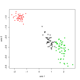
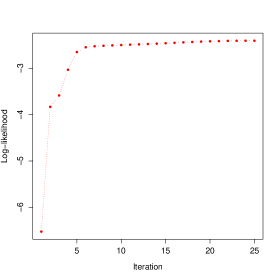
Figure 3: Projection of clustered Iris data into the latent discriminative subspace with Fisher-EM (left) and evolution of the associated log-likelihood (right).

OLDA Fisher-EM cluster cluster class 1 2 3 class 1 2 3 Setosa 50 0 0 Setosa 50 0 0 Versicolor 0 48 2 Versicolor 0 47 3 Virginica 0 1 49 Virginica 0 0 50 Misclassification rate = 0.02 Misclassification rate = 0.02

Table 2: Confusion tables for the iris data with OLDA method (supervised) and Fisher-EM (unsupervised).

	OLDA		Fisher-EM
	axis		axis
variable	1	2	1	2
sepal length	0.209	0.044	-0.203	-0.108
sepal width	0.386	0.665	-0.422	0.088
petal length	-0.554	-0.356	0.602	0.736
petal width	-0.707	0.655	0.646	-0.662

Table 3: Fisher axes estimated in the supervised case (OLDA) and in the unsupervised case (Fisher-EM).

In this first experiment, Fisher-EM has been applied to the iris data (of course, the labels have been used only for performance evaluation) and the Fisher-EM results will be compared to the ones obtained in the supervised case with the orthogonal linear analysis method (OLDA) [52]. The left panel of Figure 3 stands for the projection of the irises in the estimated discriminative space with Fisher-EM and the right panel shows the evolution of the log-likelihood on $25$ iterations until convergence. First of all, it can be observed that the estimated latent space discriminates almost perfectly the three different groups. For this experiment, the clustering accuracy has reached $98\%$ with the DLM${}_{[\alpha_{k}\beta]}$ model of Fisher-EM. Secondly, the right panel shows the monotonicity of the evolution of the log-likelihood and the convergence of the algorithm to a stationary state. Table 2 presents the confusion matrices for the partitions obtained with supervised and unsupervised classification methods. OLDA has been used for the supervised case (reclassification of the learning data) whereas Fisher-EM has provided the clustering results. One can observe that the obtained partitions induced by both methods is almost the same. This confirms that Fisher-EM has correctly modeled both the discriminative subspace and the groups within the subspace. It is also interesting to look at the loadings provided by both methods. Table 3 stands for the linear coefficients of the discriminative axes estimated, on the one hand, in the supervised case (OLDA) and, on the other hand, in the unsupervised case (Fisher-EM). The first axes of each approach appear to be very similar and the scalar product of these axes is $-0.996$. This highlights the performance of the Fisher-EM algorithm in estimating the discriminative subspace of the data. Furthermore, according to these results, the $3$ groups of irises can be mainly discriminated by the petal size meaning that only one axis would be sufficient to discriminate the $3$ iris species. Besides, this interpretation turns out to be in accordance with the recent work of Trendafilov and Joliffe [50] on variable selection in discriminant analysis via the LASSO.

5.2 Simulation study: influence of the dimension

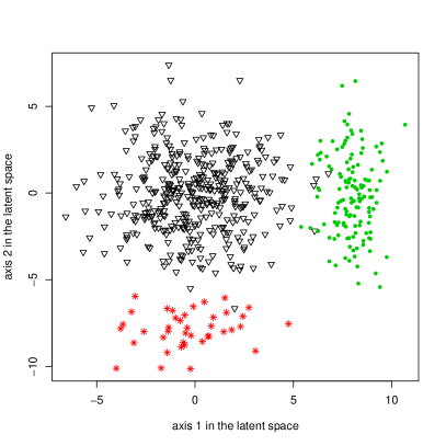
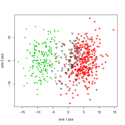
Figure 4: Visualization of the simulated data: data in their latent space (left) and data projected on the first principal components (right).

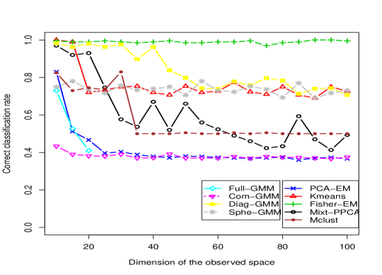
Figure 5: Influence of the dimension of the observed space on the correct classification rate for Full-GMM, PCA-EM, Com-GMM, Mixt-PPCA, k-means, Diag-GMM, Sphe-GMM and Fisher-EM algorithms.

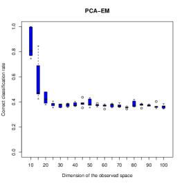
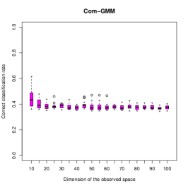
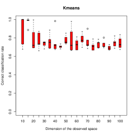
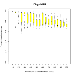
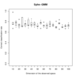
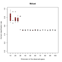
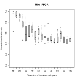
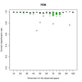
Figure 6: Boxplots of Full-GMM, PCA-EM, Com-GMM, Mixt-PPCA, k-means, Diag-GMM, Sphe-GMM and Fisher-EM algorithms.

This second experiment aims to compare with traditional methods the stability and the efficiency of the Fisher-EM algorithm in partitioning high-dimensional data. Fisher-EM is compared here with the standard EM algorithm (Full-GMM) and its parsimonious models (Diag-GMM, Sphe-GMM and Com-GMM), the EM algorithm applied in the first components of PCA explaining $90\%$ of the total variance (PCA-EM), the k-means algorithm and the mixture of probabilistic principal component analyzers (Mixt-PPCA). For this simulation, $600$ observations have been simulated following the $\mathrm{DLM}_{[\alpha_{kj}\beta_{k}]}$ model proposed in Section 3. The simulated dataset is made of $3$ unbalanced groups and each group is modeled by a Gaussian density in a $2$-dimensional space completed by orthogonal dimensions of Gaussian noise. The transformation matrix $W$ has been randomly simulated such as $W^{t}W=WW^{t}=I_{p}$ and, for this experience, the dimension of the observed space varies from $5$ to $100$. The left panel of Figure 4 shows the simulated data in their $2$-dimensional latent space whereas the right panel presents the projection of $50$-dimensional observed data on the two first axes of PCA in the observed space. As one can observe, the representation of the data on the two first principal components is actually not well suited for clustering these data while it exists a representation which discriminates perfectly the three groups. Moreover, to make the results of each method comparable, the same randomized initialization has been used for the $8$ algorithms. The experimental process has been repeated $20$ times for each dimension of the observed space in order to see both the average performances and their variances. Figure 5 presents the evolution of the clustering accuracy of each method (EM, PCA-EM, k-means, Mixt-PPCA, Fisher-EM, Diag-GMM, Sphe-GMM and Com-GMM) according to the data dimensionality and Figure 6 presents their respective boxplots. First of all, it can be observed that the Full-GMM, PCA-EM and Com-GMM have their performances which decrease quickly when the dimension increases. In fact, the Full-GMM model does not work upon the $15$th dimension and still remains unstable in a low dimensional space as well as the Com-GMM model. Similarly, the performances of PCA-EM fall down as the $10$th dimension. This can be explained by the fact that the latent subspace provided by PCA does not allow to well discriminate the groups, as already suggested by Figure 4. However, the PCA-EM approach can be used whatever the dimension is whereas Full-GMM cannot be used as the $20$th dimension because of numerical problems linked to singularity of the covariance matrices. Moreover, their boxplots show a large variation on the clustering accuracy. Secondly, Sphe-GMM, Diag-GMM and k-means present the same trend with high performances in low-dimensional spaces which decrease until they reach a clustering accuracy of $0.75$. Diag-GMM seems however to resist a little bit more than k-means to the dimension increasing. Mixt-PPCA and Mclust both follow the same tendency as the previous methods but from the $30$th dimension their performances fall down until the clustering accuracy reaches $0.5$. The poor performances of Mixt-PPCA can be explained by the fact that Mixt-PPCA models each group in a different subspace whereas the model used for simulating the observations assumes a common discriminative subspace. Finally, Fisher-EM appears to be more effective than the other methods and, more importantly, it remains very stable while the data dimensionality increases. Furthermore, the boxplot associated with the Fisher-EM results suggests that it is a steady algorithm which succeeds in finding out the discriminative latent subspace of the data even with random initializations.

5.3 Simulation study: model selection

This last experiment on simulations aims to study the performance of BIC for both model and component number selection. For this experiment, $4$ Gaussian components of $75$ observations each have been simulated according to the DLM${}_{[\alpha_{k}\beta]}$ model in a $3$-dimensional space completed by 47 orthogonal dimensions of Gaussian noise (the dimension of the observation space is therefore $p=50$). The transformation matrix $W$ has been again randomly simulated such as $W^{t}W=WW^{t}=I_{p}$. Table 4 presents the BIC values for the family of DLM models and, in a comparative purpose, the BIC values for 7 other methods already used in the last experiments: EM with the Full-GMM, Diag-GMM, Sphe-GMM and Com-GMM models, Mixt-PPCA, Mclust [20] (with model [EEE] which is the most appropriate model for these data) and PCA-EM. Moreover, BIC is computed for different partition numbers varying between 2 and 6 clusters. First of all, one can observe that the BIC values linked to the models which are different from the DLM model are very low compared to the DLM models. This suggests that the models which best fit the data are the DLM models. Secondly, 8 of the 12 DLM models select the right number of components ($K=4$). In particular, the DLM models which assume a common variance between each cluster outside the latent subspace (models DLM_[.β]) all select the 4 clusters. The other methods under-estimate the number of clusters. BIC has the largest value for the DLM${}_{[\alpha_{k}\beta]}$ model with $4$ components which is actually the model used for simulating the data. Finally, the right-hand side of Figure 7 presents the projection of the data on the discriminative subspace of $3$ dimensions estimated by Fisher-EM with the DLM${}_{[\alpha_{k}\beta]}$ model whereas the left-hand side figure represents the projection of the data on the $3$ first principal components of PCA. As one can observe, in the PCA case, the axes separate only 2 groups, which is in accordance with the model selection pointed out by BIC for this method. Conversely, in the Fisher-EM case, the 3 discriminative axes separate well the $4$ groups and such a representation could clearly help the practitioner in understanding the clustering results.

	number of components
methods	2	3	4	5	6
DLM${}_{[\Sigma_{k}\beta_{k}]}$	-114.6172	-114.5996	-115.4875	-115.6439	-116.7350
DLM${}_{[\Sigma_{k}\beta]}$	-116.9006	-117.4791	-115.0215	-116.0837	-116.8912
DLM${}_{[\Sigma\beta_{k}]}$	-116.9007	-116.9568	-118.5480	-119.3458	-120.0418
DLM[Σβ]	-120.9006	-120.2496	-119.8787	-120.6301	-120.6166
DLM${}_{[\alpha_{kj}\beta_{k}]}$	-116.5750	-114.9578	-114.7986	-115.6658	-116.5750
DLM${}_{[\alpha_{kj}\beta]}$	-121.8565	-117.4968	-115.1525	-115.8571	-117.7598
DLM${}_{[\alpha_{k}\beta_{k}]}$	-115.2290	-115.0808	-114.7934	-115.6603	-116.5027
DLM${}_{[\alpha_{k}\beta]}$	-121.8565	-117.6217	-114.1471	-115.7909	-116.6739
DLM${}_{[\alpha_{j}\beta_{k}]}$	-116.7295	-118.4031	-119.2610	-120.7783	-122.0415
DLM${}_{[\alpha_{j}\beta]}$	-123.3448	-120.9052	-120.4578	-121.1248	-121.9098
DLM${}_{[\alpha\beta_{k}]}$	-118.7295	-118.3865	-119.7309	-121.5124	-123.1506
DLM[αβ]	-123.3443	-120.8989	-120.4347	-121.7451	-123.2730
Full-GMM	-177.6835	-252.8908	-440.6805	-3005.531	-4367.653
Com-GMM	-150.0518	-193.0624	-231.4546	-270.2741	-309.7809
Mixt-PPCA	-151.1561	-176.3615	-201.5709	-226.7789	-251.9931
Diag-GMM	-189.8663	-262.7929	-419.360	-407.2755	-466.6955
Sphe-GMM	-190.9812	-258.3534	-302.8030	-382.7666	-433.3845
PCA-EM	-127.0857	-173.7174	-247.3894	-364.9811	-594.4000
Mclust[EII]	-229.3360	-229.3024	-230.0155	-230.8431	-231.5140

Table 4: BIC values for model selection.

Projection on the 3 first principal components	Projection on the discriminative axes estimated by Fisher-EM

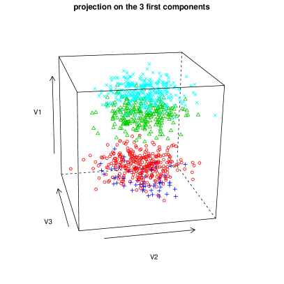
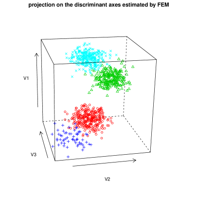
Figure 7: Projection of the data in the 3 first principal components of PCA (left) and in the discriminant subspace estimated by Fisher-EM with the DLM${}_{[\alpha_{k}\beta]}.$

5.4 Real data set benchmark

This last experimental paragraph will focus on comparing on real-world datasets the efficiency of Fisher-EM with several linear and nonlinear existing methods, including the most recent ones. On the one hand, Fisher-EM will be compared to the 8 already used clustering methods: EM with the Full-GMM, Diag-GMM, Sphe-GMM and Com-GMM models, Mixt-PPCA, Mclust (with its most adapted model for these data), PCA-EM and k-means. On the other hand, the new Fisher-EM challengers will be k-means computed on the two first components of PCA (PCA–k-means), an heteroscedastic factor mixture analyzer (HMFA) method [43] and three discriminative versions of k-means: LDA–k-means [16], Dis–k-means and DisCluster (see [53] for more details). The comparison has been made on $7$ different benchmark datasets coming mostly from the UCI machine learning repository:

• The chironomus data contain $148$ larvae which are split up into $3$ species and described by $17$ morphometric attributes. This dataset is described in detailed in [43].

• The wine dataset is composed by $178$ observations which are split up into $3$ classes and characterized by $13$ variables.

• The iris dataset which is made of $3$ different groups and described by $4$ variables. This dataset has been described in detail in Section 5.1.

• The zoo dataset includes $7$ families of $101$ animals characterized by $16$ variables.

• The glass data are composed by $214$ observations belonging to $6$ different groups and described by $7$ variables.

• The $4435$ satellite images are split up into $6$ classes and are described by $36$ variables.

• Finally, the last dataset is the USPS data where only the classes which are difficult to discriminate are considered. Consequently, this dataset consists of 1756 records (rows) and 256 attributes divided in $3$ classes (numbers 3, 5 and 8).

Table 5 presents the average clustering accuracies and the associated standard deviations obtained for the $12$ DLM models and for the methods already used in the previous experiments. The results for the $19$ first methods of the table have been obtained by averaging $20$ trials with random initializations except for Mclust which has its own deterministic initialization and this explains the lack of standard deviation for Mclust. Similarly, Table 6 provides the clustering accuracies found in the literature for the recent methods on the same datasets. It is important to notice that the results of Table 6 have been obtained in slightly different benchmarking situations. Missing values in Table 5 are due to non-convergence of the algorithms whereas missing values in Table 6 are due to the unavailability of the information for the concerned method. First of all, one can remark that Fisher-EM outperforms the other methods for most of the UCI datasets such as wine, iris, zoo, glass, satimage and usps358 datasets. Finally, it is interesting from a practical point of view to notice that some DLM models work well in most situations. In particular, the DLM_[.β] models, in which the variance outside the discriminant subspace is common to all groups, provide very satisfying results for all the datasets considered here.

Method	iris	wine	chironomus	zoo	glass	satimage	usps358
DLM${}_{[\Sigma_{k}\beta_{k}]}$	94.8$\pm 2.3$	96.1$\pm 0.0$	91.7$\pm 5.2$	-	39.5$\pm 1.8$	64.6$\pm 2.2$	77.9$\pm 7.1$
DLM${}_{[\Sigma_{k}\beta]}$	96.7$\pm 0.0$	95.5$\pm 0.0$	97.2$\pm 0.1$	-	39.9$\pm 1.4$	65.7$\pm 0.8$	70.0$\pm 8.5$
DLM${}_{[\Sigma\beta_{k}]}$	81.9$\pm 2.4$	94.1$\pm 1.3$	91.8$\pm 2.4$	73.3$\pm 5.5$	40.6$\pm 0.9$	62.7$\pm 1.9$	74.1$\pm 9.4$
DLM[Σβ]	77.8$\pm 3.7$	93.6$\pm 1.6$	89.1$\pm 6.3$	78.4$\pm 6.4$	38.5$\pm 1.9$	68.0$\pm 1.7$	66.4$\pm 8.7$
DLM${}_{[\alpha_{kj}\beta_{k}]}$	89.3$\pm 0.0$	95.5$\pm 0.0$	86.1$\pm 6.3$	73.7$\pm 3.5$	42.0$\pm 2.2$	65.5$\pm 2.0$	74.8$\pm 9.1$
DLM${}_{[\alpha_{kj}\beta]}$	91.1$\pm 1.4$	94.2$\pm 0.2$	96.3$\pm 7.0$	70.4$\pm 5.3$	40.1$\pm 3.3$	65.0$\pm 2.9$	68.7$\pm 11.1$
DLM${}_{[\alpha_{k}\beta_{k}]}$	96.1$\pm 2.2$	95.5$\pm 0.0$	87.5$\pm 3.9$	73.7$\pm 3.6$	39.2$\pm 3.7$	64.4$\pm 2.1$	76.2$\pm 7.6$
DLM${}_{[\alpha_{k}\beta]}$	98.0$\pm 0.0$	94.3$\pm 0.0$	96.2$\pm 6.8$	72.8$\pm 3.1$	40.1$\pm 2.0$	58.9$\pm 5.3$	74.1$\pm 10.6$
DLM${}_{[\alpha_{j}\beta_{k}]}$	79.3$\pm 3.6$	93.8$\pm 2.8$	83.7$\pm 3.9$	72.5$\pm 7.0$	39.4$\pm 0.9$	62.4$\pm 1.8$	77.8$\pm 8.2$
DLM${}_{[\alpha_{j}\beta]}$	72.7$\pm 6.5$	92.6$\pm 3.2$	89.7$\pm 6.3$	80.1$\pm 4.2$	39.5$\pm 1.5$	68.0$\pm 1.5$	74.2$\pm 11.2$
DLM${}_{[\alpha\beta_{k}]}$	80.3$\pm 4.3$	96.3$\pm 1.9$	83.6$\pm 8.5$	70.2$\pm 7.0$	39.1$\pm 2.4$	62.4$\pm 2.5$	81.2$\pm 6.5$
DLM[αβ]	79.8$\pm 4.0$	97.1$\pm 0.0$	89.8$\pm 6.6$	78.0$\pm 4.8$	38.4$\pm 1.3$	67.9$\pm 1.3$	72.8$\pm 9.8$
Full-GMM	79.0$\pm 5.7$	60.9$\pm 7.7$	44.8$\pm 4.1$	-	38.3$\pm 2.1$	35.9$\pm 3.1$	-
Com-GMM	57.6$\pm 18.3$	61.0$\pm 14.9$	51.9$\pm 10.9$	59.9$\pm 10.3$	38.3$\pm 3.1$	26.1$\pm 1.5$	38.2$\pm 1.1$
Mixt-PPCA	89.1$\pm 4.2$	63.1$\pm 7.9$	56.3$\pm 4.5$	50.9$\pm 6.5$	37.0$\pm 2.3$	40.6$\pm 4.7$	53.1$\pm 9.6$
Diag-GMM	93.5$\pm 1.3$	94.6$\pm 2.8$	92.1$\pm 4.2$	70.9$\pm 12.3$	39.1$\pm 2.4$	60.8$\pm 5.2$	45.9$\pm 9.1$
Sphe-GMM	89.4$\pm 0.4$	96.6$\pm 0.0$	85.9$\pm 9.9$	69.4$\pm 5.4$	37.0$\pm 2.1$	60.2$\pm 7.5$	78.7$\pm 11.2$
PCA-EM	66.9$\pm 9.9$	64.4$\pm 5.7$	66.1$\pm 4.0$	61.9$\pm 6.2$	39.0$\pm 1.7$	56.2$\pm 4.2$	67.6$\pm 11.2$
k-means	88.7$\pm 4.0$	95.9$\pm 4.0$	92.9$\pm 6.0$	68.0$\pm 7.4$	41.3$\pm 2.8$	66.6$\pm 4.1$	74.9$\pm 13.9$
Mclust	96.7	97.1	97.9	65.3	41.6	58.7	55.5
Model name	(VEV)	(VVI)	(EEE)	(EII)	(VEV)	(VVV)	(EEE)

Table 5: Clustering accuracies and their standard deviations (in percentage) on the UCI datasets averaged on 20 trials. No standard deviation is reported for Mclust since its initialization procedure is deterministic and always provides the same initial partition.

Method	wine	iris	chironomus	zoo	glass	satimage	usps358
PCA–k-means [16]	70.2	88.7	-	79.2	47.2	-	-
LDA–k-means [16]	82.6	98.0	-	84.2	51.0	-	-
Dis–k-means [53]	-	-	-	-	-	65.1	-
DisCluster [53]	-	-	-	-	-	64.2	-
HMFA [43]	-	-	98.7	-	-	-	-

Table 6: Clustering accuracies (in percentage) on UCI datasets found in the literature (these results have been obtained with slightly different experimental setups).

6 Application to mass spectrometry

In this last experimental section, the Fisher-EM procedure is applied to the problem of cancer detection using MALDI mass spectrometry. MALDI mass spectrometry is a non-invasive biochemical technique which is useful in searching for disease biomarkers, assessing tumor progression or evaluating the efficiency of drug treatment, to name just a few applications. In particular, a promising field of application is the early detection of the colorectal cancer, which is one of the principal causes of cancer-related mortality, and MALDI imaging could in few years avoid in some cases the colonoscopy method which is invasive and quite expensive.

6.1 Data and experimental setup

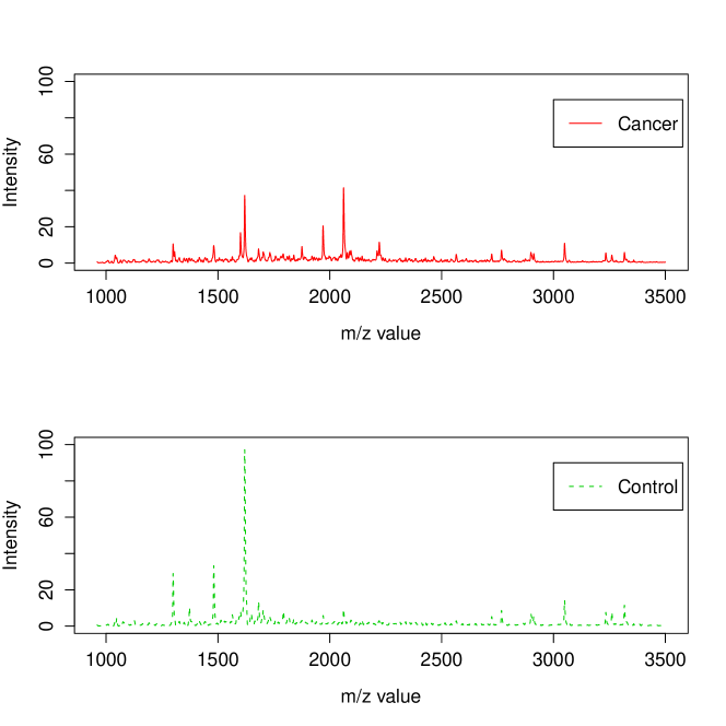
Figure 8: Estimated mean spectra of the cancer class (up) and of the control class (bottom) on the m/z interval 900–3500 Da.

The MALDI2009 dataset has been provided by Theodore Alexandrov from the Center for Industrial Mathematics (University of Bremen, Germany) and is made of 112 spectra of length 16 331. Among the 112 spectra, 64 are spectra from patients with the colorectal cancer (referred to as cancer hereafter) and 48 are spectra from healthy persons (referred to as control). Each of the 112 spectra is a high-dimensional vector of 16 331 dimensions which covers the mass-to-charge (m/z) ratios from 960 to 11 163 Da. For further reading, the dataset is presented in detail and analyzed in a supervised classification framework in [3].

Following the experimental protocol of [3], Fisher-EM was applied on the 6 168 dimensions corresponding to m/z ratios between 960 and 3 500 Da since there is no discriminative information on the reminder. Figure 8 shows the mean spectra of the cancer and control classes estimated by Fisher-EM on the m/z interval 900–3500 Da. To be able to compare the clustering results of Fisher-EM, PCA-EM and mixture of PPCA (Mixt-PPCA) have been applied to this subset as well. It has been asked to all methods to cluster the dataset into 2 groups. It is important to remark that this clustering problem is a $n\ll p$ problem and, among the model-based methods, only these three methods are able to deal with it (see Section 4.6).

6.2 Experimental results

PCA-EM
	Cluster
Class	Cancer	Control
Cancer	48	16
Control	1	47
Misclassification rate = 0.15

Mixt-PPCA
	Cluster
Class	Cancer	Control
Cancer	62	2
Control	10	38
Misclassification rate = 0.11

Fisher-EM
	Cluster
Class	Cancer	Control
Cancer	57	7
Control	3	45
Misclassification rate = 0.09

Table 7: Confusion tables for PCA-EM (left), mixture of PPCA (center) and Fisher-EM (right).

Table 7 presents the confusion tables computed from the clustering results of PCA-EM, mixture of PPCA and Fisher-EM. On the one hand, PCA-EM has selected $d=4$ principal axes with the 90% variance rule before to cluster the data in this subspace and mixture of PPCA has selected $d=2$ principal axes for each group. On the other hand, Fisher-EM has estimated the discriminative latent subspace with $d=K-1=1$ axis to cluster this high-dimensional dataset. It first appears that PCA-EM and mixture of PPCA provide satisfying clustering results on such a complex dataset. However, it is disappointing to see that the PCA-EM make a significant number of false negatives (cancers classified as non-cancers) since the classification risk is not symmetric here. Conversely, mixture of PPCA and Fisher-EM provide a better clustering results both from a global point of view (respectively 89% and 91% of clustering accuracy) and from a medical point of view since Fisher-EM makes significantly less false negatives with an acceptable number of false positives.

More importantly, Fisher-EM provides information which can be interpreted a posteriori to better understand both the data and the phenomenon. Indeed, the values of the estimated loading matrix $U$, which is a $6\,168\times 1$ matrix here, expressed the correlation between the discriminative subspace and the original variables. It is therefore possible to identify the original variables with the highest power of discrimination. It is important to highlight that Fisher-EM extracts this information from the data in a unsupervised framework. Figure 9 shows the correlation between each original variable and the discriminative subspace on an arbitrary scale. The peaks of this curve correspond to the original variables which have a high correlation with the discriminative axis estimated by Fisher-EM.

Figure 10 plots the difference between the mean spectra of the classes cancer and control (cancer - control) and indicates as well, using red triangles, the most discriminative original variables (m/z values). It is not surprising to see that original variables where the cancer and control spectra have a big difference are among the most discriminative. More surprisingly, Fisher-EM selects the original variables with m/z values equal to 2800 and 3050 as discriminative variables whereas the difference between cancer and control spectra is less for these variables than the difference on the variable with m/z value equal to 1350. Such information, which have extracted from the data in a unsupervised framework, may help the practitioner to understand the clustering results.

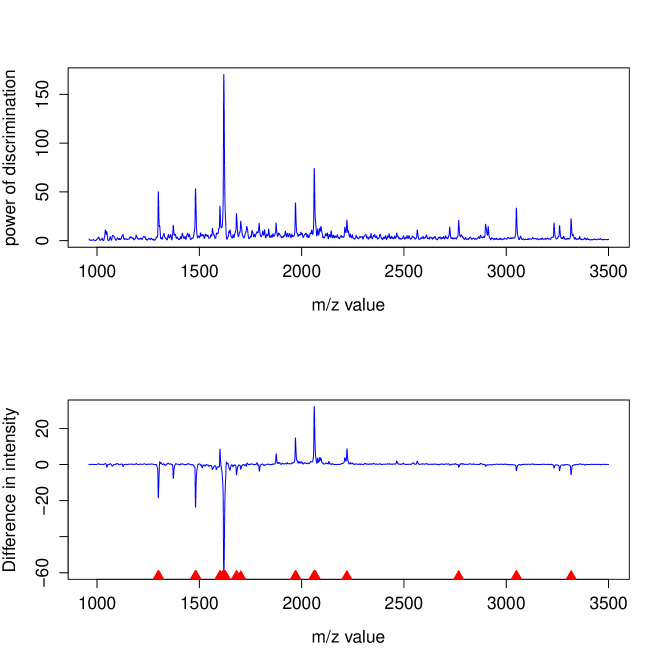
Figure 9: Discrimination power of the original variables: correlation between original variables and the discriminative subspace on an arbitrary scale.

Figure 10: Difference between the mean spectra of the classes cancer and control (cancer - control) and most discriminative variables (indicated by red triangles).

7 Conclusion and further works

This work has presented a discriminative latent mixture model which models the data in a latent orthonormal discriminative subspace with an intrinsic dimension lower than the dimension of the original space. A family of 12 parsimonious DLM models has been exhibited by constraining model parameters within and between groups. An estimation algorithm, called the Fisher-EM algorithm, has been also proposed for estimating both the mixture parameters and the latent discriminative subspace. The determination procedure for the discriminative subspace adapts the well-known Fisher criterion to the unsupervised classification context under an orthonormality constraint. Furthermore, when the number of groups is not too large, the estimated discriminative subspace allows a useful projection of the clustered data. Experiments on simulated and real datasets have shown that Fisher-EM performs better than existing clustering methods. The Fisher-EM algorithm has been also applied to the clustering of mass spectrometry data, which is a real-world and complex application. In this specific context, Fisher-EM has shown its ability to both efficiently cluster high-dimensional mass spectrometry data and give a pertinent interpretation of the results.

However, the convergence of the Fisher-EM algorithm has been proved in this work only for 2 of the DLM models and the convergence for other models should be investigated. We feel that the convergence could be proved for these models at least in a generalized EM context. Among the other possible extensions of this work, it could be interesting to find a way to visualize in 2D or 3D the clustered data when the estimated discriminative subspace has more than 4 dimensions. Another extension could be to consider a kernel version of Fisher-EM. For this, it would be necessary to replace the Gram matrix introduced in Section 4.6 by a kernel. Finally, it could be also interesting to introduce sparsity in the loading matrix through a $\ell_{1}$ penalty in order to ease the interpretation of the discriminative axes.

Appendix A Appendix

In order not to surcharge the notations, the index $q$ of the current iteration of the Fisher-EM algorithm is not indicated in the following proofs. We also define the matrices $\tilde{W}$ and $\bar{W}$ such that $W=\tilde{W}+\bar{W}$. The matrix $\tilde{W}$ is defined as a $p\times p$ matrix containing the $d$ first vectors of $W$ completed by zeros such as $\tilde{W}=[U,0_{p-d}]$ and $\bar{W}=W-\tilde{W}$ is defined by $\bar{W}=[0_{d},V]$.

A.1 E step

Proof of Proposition 1.

The conditional expectation $t_{ik}=E[P(z_{ik}|y_{i},\Theta)]$ can be viewed as well as the posterior probability of the observation $y_{i}$ given a group $k$ and, thanks to the Bayes’ formula, can be written:

$$t_{ik}=\frac{\pi_{k}\phi(y_{i},\theta_{k})}{\sum_{l=1}^{K}\pi_{l}\phi(y_{i},\theta_{l})},$$ (A.1)

where $\phi$ is the Gaussian density, and $\pi_{k}$ and $\theta_{k}$ are the parameters of the $k$th mixture component estimated in the previous iteration. This posterior probability $t_{ik}$ can also be formulated from the cost function $\Gamma_{k}$ such that:

$$t_{ik}=\frac{1}{\sum_{l=1}^{K}\exp\left(\frac{1}{2}(\Gamma_{k}(y_{i})-\Gamma_{l}(y_{i}))\right)},$$ (A.2)

where $\Gamma_{k}(y_{i})=-2\log(\pi_{k}\phi(y_{i},\theta_{k}))$. According to the assumptions of the model $\mathrm{DLM}_{[\Sigma_{k}\beta_{k}]}$ and given that $W=\tilde{W}+\bar{W}$, $\Gamma_{k}$ can be reformulated as:

$$\begin{split}\Gamma_{k}(y_{i})=&\quad(y_{i}-m_{k})^{t}\tilde{W}\Delta_{k}^{-1}\tilde{W}^{t}(y_{i}-m_{k})+(y_{i}-m_{k})^{t}\bar{W}\Delta_{k}^{-1}\bar{W}^{t}(y_{i}-m_{k})\\ &+\log(|\Delta_{k}|)-2\log(\pi_{k})+p\leavevmode\nobreak\ \log(2\pi),\end{split}$$ (A.3)

Moreover, since the relations $\tilde{W}(\tilde{W}^{t}\tilde{W})=\tilde{W}$ and $\bar{W}(\bar{W}^{t}\bar{W})=\bar{W}$ hold due to the construction of $\tilde{W}$ and $\bar{W}$, then:

$$\begin{split}\Gamma_{k}(y_{i})=&\quad\left(\tilde{W}\tilde{W}^{t}(y_{i}-m_{k})\right)^{t}\tilde{W}\Delta_{k}^{-1}\tilde{W}^{t}\left(\tilde{W}\tilde{W}^{t}(y_{i}-m_{k})\right)\\ &+\frac{1}{\beta_{k}}\left(\bar{W}\bar{W}^{t}(y_{i}-m_{k})\right)^{t}\left(\bar{W}\bar{W}^{t}(y_{i}-m_{k})\right)\\ &+\log(|\Delta_{k}|)-2\log(\pi_{k})+p\leavevmode\nobreak\ \log(2\pi).\end{split}$$ (A.4)

Let us now define $\vartheta_{k}=\tilde{W}\Delta_{k}^{-1}\tilde{W}^{t}$ and $||.||_{\vartheta_{k}}$, a norm on the latent space spanned by $\tilde{W}$, such that $||y||_{\vartheta_{k}}^{2}=y^{t}\vartheta_{k}y$. With these notations, and according to the definition of $\Delta_{k}$, $\Gamma_{k}$ can be rewritten as:

$$\begin{split}\Gamma_{k}(y_{i})=&\quad||\tilde{W}\tilde{W}^{t}(y_{i}-m_{k})||_{\vartheta_{k}}^{2}+\frac{1}{\beta_{k}}||\bar{W}\bar{W}^{t}(y_{i}-m_{k})||^{2}\\ &+\log(\left|\Sigma_{k}\right|)+(p-d)\leavevmode\nobreak\ \log(\beta_{k})-2\log(\pi_{k})+p\leavevmode\nobreak\ \log(2\pi).\end{split}$$ (A.5)

Let us also define the projection operators $P$ and $P^{\perp}$ on the subspaces $\mathbb{E}$ and $\mathbb{E}^{\perp}$ respectively:

• $P(y)=\tilde{W}\tilde{W}^{t}y$ is the projection of $y$ on the discriminative space $\mathbb{E}$,

• $P^{\perp}(y)=\bar{W}\bar{W}^{t}y$ is the projection of $y$ on the complementary space $\mathbb{E}^{\perp}$.

Consequently, the cost function $\Gamma_{k}$ can be finally reformulated as:

$$\begin{split}\Gamma_{k}(y_{i})=&\quad\left\|P(y_{i}-m_{k})\right\|{}_{\vartheta_{k}}^{2}+\frac{1}{\beta_{k}}\left\|P^{\perp}(y_{i}-m_{k})\right\|{}^{2}\\ &+\log(\left|\Sigma_{k}\right|)+(p-d)\leavevmode\nobreak\ \log(\beta_{k})-2\log(\pi_{k})+p\leavevmode\nobreak\ \log(2\pi).\end{split}$$ (A.6)

Since $P^{\perp}(y)=y-P(y)$, then the distance associated with the complementary subspace can be rewritten as $||P^{\perp}(y_{i}-m_{k})||^{2}=||(y_{i}-m_{k})-P(y_{i}-m_{k})||^{2}$ and this allow to conclude. ∎

A.2 M step

Proof of Proposition 2.

In the case of the model $\mathrm{DLM}_{[\Sigma_{k}\beta_{k}]}$, at iteration $q$, the conditional expectation of the complete log-likelihood $Q(y_{1},\dots,y_{n},\theta|\theta^{(q-1)})$ of the observed data $\{y_{1},\dots,y_{n}\}$ has the following form:

$$\begin{split}Q(\theta)=&\sum_{i=1}^{n}\sum_{k=1}^{K}t_{ik}\log(\pi_{k}\phi(y_{i},\theta_{k}))\\ =&\sum_{i=1}^{n}\sum_{k=1}^{K}t_{ik}\Bigl{[}-\frac{1}{2}\log(|S_{k}|)-\frac{1}{2}(y_{i}-m_{k})^{t}S_{k}^{-1}(y_{i}-m_{k})+\log(\pi_{k})-\frac{p}{2}\leavevmode\nobreak\ \log(2\pi)\Bigr{]},\end{split}$$ (A.7)

where $t_{ik}=E[z_{ik}|\theta^{(q-1)}]$. According to the definitions of the diagonal matrix $\Delta_{k}$ and of the orientation matrix $W$ for which $W^{-1}=W^{t}$, the inverse covariance matrix $S_{k}^{-1}$ of $Y$ can be written as $S_{k}^{-1}=(W\Delta_{k}W^{t})^{-1}=W^{-t}\Delta_{k}^{-1}W^{-1}=W\Delta_{k}^{-1}W^{t}$ and the determinant of $S_{k}$ can be also reformulated in the following way:

$$|S_{k}|=|\Delta_{k}|=\left|\Sigma_{k}\right|\beta_{k}^{p-d}.$$ (A.8)

Consequently, the complete log-likelihood $Q(\theta)$ can be rewritten as:

$$\begin{split}Q(\theta)=&-\frac{1}{2}\sum_{k=1}^{K}n_{k}\Bigl{[}-2\log(\pi_{k})+\log(\left|\Sigma_{k}\right|)+(p-d)\leavevmode\nobreak\ \log(\beta_{k})\\ &+\frac{1}{n_{k}}\sum_{i=1}^{n}t_{ik}(y_{i}-m_{k})^{t}W\Delta_{k}^{-1}W^{t}(y_{i}-m_{k})+\gamma\Bigr{]}.\end{split}$$ (A.9)

where $n_{k}=\sum_{i=1}^{n}t_{ik}$ and $\gamma=p\log(2\pi)$ is a constant term. At this point, two remarks can be done on the quantity $\sum_{i=1}^{n}t_{ik}(y_{i}-m_{k})^{t}W\Delta_{k}^{-1}W^{t}(y_{i}-m_{k})$. First, as this quantity is a scalar, it is equal to its trace. Secondly, this quantity can be divided in two parts since $W=[U,V]$ and $W=\tilde{W}+\bar{W}$. Then, the relation $W\Delta_{k}^{-1}W^{t}=\tilde{W}\Delta_{k}^{-1}\tilde{W}^{t}+\bar{W}\Delta_{k}^{-1}\bar{W}^{t}$ is stated and we can write:

$$\begin{array}[]{ccc}(y_{i}-m_{k})^{t}W\Delta_{k}^{-1}W^{t}(y_{i}-m_{k})&=&\mathrm{trace}\left((y_{i}-m_{k})^{t}\tilde{W}\Delta_{k}^{-1}\tilde{W}^{t}(y_{i}-m_{k})\right)\\ &&+\quad\mathrm{trace}\left((y_{i}-m_{k})^{t}\bar{W}\Delta_{k}^{-1}\bar{W}^{t}(y_{i}-m_{k})\right).\end{array}$$ (A.10)

Moreover, pointing out that $C_{k}=\frac{1}{n_{k}}\sum_{i=1}^{n}t_{ik}(y_{i}-m_{k})(y_{i}-m_{k})^{t}$ is the empirical covariance matrix the $k$th group, the previous quantity can be rewritten as:

$$\frac{1}{n_{k}}\sum_{i=1}^{n}t_{ik}(y_{i}-m_{k})^{t}W\Delta_{k}^{-1}W^{t}(y_{i}-m_{k})=\mathrm{trace}(\Delta_{k}^{-1}\tilde{W}^{t}C_{k}\tilde{W})+\mathrm{trace}(\Delta_{k}^{-1}\bar{W}^{t}C_{k}\bar{W})$$ (A.11)

and finally:

$$\frac{1}{n_{k}}\sum_{i=1}^{n}t_{ik}(y_{i}-m_{k})^{t}W\Delta_{k}^{-1}W^{t}(y_{i}-m_{k})=\quad\mathrm{trace}(\Sigma_{k}^{-1}U^{t}C_{k}U)\quad+\quad\sum_{j=1}^{p-d}\frac{v_{j}^{t}C_{k}v_{j}}{\beta_{k}},$$ (A.12)

where $v_{j}$, is the $j$th column vector of $V$. However, since $\bar{W}=W-\tilde{W}$ and $W=[U,V]$, it is also possible to write:

$$\begin{split}\frac{1}{\beta_{k}}\sum_{j=1}^{p-d}v_{j}^{t}C_{k}v_{j}=&\frac{1}{\beta_{k}}\left(\sum_{j=1}^{p}w_{j}^{t}C_{k}w_{j}-\sum_{j=1}^{d}u_{j}^{t}C_{k}u_{j}\right)\\ =&\frac{1}{\beta_{k}}\left(\sum_{j=1}^{p}\mathrm{trace}(w_{j}w_{j}^{t}C_{k})-\sum_{j=1}^{d}u_{j}^{t}C_{k}u_{j}\right)\\ =&\frac{1}{\beta_{k}}\Bigl{[}\mathrm{trace}(C_{k})-\sum_{j=1}^{d}u_{j}^{t}C_{k}u_{j}\Bigr{]}.\end{split}$$ (A.13)

Consequently, replacing this quantity in (A.9) provides the final expression of $Q(\theta)$. ∎

Proof of Proposition 3.

The maximization of $Q(\theta)$ conduces for the DLM models to the following estimates.

Estimation of $\mathbf{\pi_{k}}$

The prior probability $\pi_{k}$ of the group $k$ can be estimated by maximizing $Q(\theta)$ with respect to the constraint $\sum_{k=1}^{K}\pi_{k}=1$ which is equivalent to maximize the Lagrange function:

$$L=Q(\theta)+\lambda\left(\sum_{k=1}^{K}\pi_{k}-1\right),$$ (A.14)

where $\lambda$ is the Lagrange multiplier. Then, the partial derivative of $L$ with respect to $\pi_{k}$ is $\frac{\partial L}{\partial\pi_{k}}=\frac{n_{k}}{\pi_{k}}+\lambda.$ Consequently:

$$\forall k=1,\dots,K\qquad\frac{\partial L}{\partial\pi_{k}}=0\Longleftrightarrow\frac{n_{k}}{\pi_{k}}+\lambda=0\Longleftrightarrow n_{k}+\lambda\pi_{k}=0,$$ (A.15)

and:

$$\sum_{k=1}^{K}(n_{k}+\lambda\pi_{k})=n+\lambda=0\Longrightarrow\lambda=-n.$$ (A.16)

Replacing $\lambda$ by its value in the partial derivative conduces to an estimation of $\pi_{k}$ by:

$$\hat{\pi}_{k}=\frac{n_{k}}{n}.$$ (A.17)

Estimation of $\mathbf{\mu_{k}}$

The mean $\mu_{k}$ of the $k$th group in the latent space can be also estimated by maximizing the expectation of the complete log-likelihood (equation A.7), which can be written in the following way:

$$Q(\theta)=\sum_{i=1}^{n}\sum_{k=1}^{K}t_{ik}\Bigl{[}-\frac{1}{2}\log(|S_{k}|)-\frac{1}{2}(y_{i}-U\mu_{k})^{t}S_{k}^{-1}(y_{i}-U\mu_{k})+\log(\pi_{k})-\frac{p}{2}\log(2\pi)\Bigr{]}.$$ (A.18)

Consequently, the partial derivative of $Q$ with respect to $\mu_{k}$ is $\frac{\partial Q(\theta)}{\partial\mu_{k}}=-\frac{1}{2}\sum_{i=1}^{n}t_{ik}U^{t}(y_{i}-U\mu_{k}).$ Setting this quantity to $0$ gives:

$$\frac{\partial Q(\theta)}{\partial\mu_{k}}=0\Longleftrightarrow\sum_{i=1}^{n}t_{ik}U^{t}y_{i}=\sum_{i=1}^{n}t_{ik}\mu_{k}.$$ (A.19)

and conduces to:

$$\hat{\mu}_{k}=\frac{1}{n_{k}}\sum_{i=1}^{n}t_{ik}U^{t}y_{i}.$$ (A.20)

Model $\mathrm{DLM}_{[\Sigma_{k}\beta_{k}]}$

From Equation (4.7), the partial derivative of $Q(\theta)$ with respect to $\Sigma_{k}$ has the following form:

$$\frac{\partial Q(\theta)}{\partial\Sigma_{k}}=-\frac{n_{k}}{2}\frac{\partial}{\partial\Sigma_{k}}\left[\log(|\Sigma_{k}|)+\mathrm{trace}\left(\Sigma_{k}^{-1}U^{t}C_{k}U\right)\right].$$ (A.21)

Using the matrix derivative formula of the logarithm of a determinant, $\frac{\partial\log(|A|)}{\partial A}=\left(A^{-1}\right)^{t}$, and of the trace of a product, $\frac{\partial\mathrm{trace}(A^{-1}B)}{\partial A}=-\left(A^{-1}BA^{-1}\right)^{t}$, the equality of $\frac{\partial Q(\theta)}{\partial\Sigma_{k}}$ to the $d\times d$ zero matrix yields to the relation:

$$\Sigma_{k}^{-1}=\Sigma_{k}^{-1}U^{t}C_{k}U\Sigma_{k}^{-1},$$ (A.22)

and, by multiplying on the left and on the right by $\Sigma_{k},$ we find out the estimate of $\Sigma_{k}$:

$$\hat{\Sigma}_{k}=U^{t}C_{k}U.$$ (A.23)

The estimation of $\beta_{k}$ is also obtained by maximizing $Q$ subject to $\beta_{k}$:

$$\frac{\partial Q(\theta)}{\beta_{k}}=0\Longleftrightarrow\frac{p-d}{\beta_{k}}-\frac{\mathrm{trace}(C_{k})}{\beta_{k}^{2}}+\frac{1}{\beta_{k}^{2}}\sum_{j=1}^{d}u_{j}^{t}C_{k}u_{j}=0,$$ (A.24)

and it is possible to conclude:

$$\hat{\beta}_{k}=\frac{\mathrm{trace}(C_{k})-\sum_{j=1}^{d}u_{j}^{t}C_{k}u_{j}}{p-d}.$$ (A.25)

Model $\mathrm{DLM}_{[\Sigma_{k}\beta]}$

In this case, $Q$ has the following form:

$$\begin{split}Q(\theta)=&-\frac{1}{2}\Bigl{(}\sum_{k=1}^{K}n_{k}\Bigl{[}-2\log(\pi_{k})+\mathrm{trace}(\Sigma_{k}^{-1}U^{t}C_{k}U)+\log(\left|\Sigma_{k}\right|)\Bigr{]}\\ &+\sum_{k=1}^{K}n_{k}(p-d)\leavevmode\nobreak\ \log(\beta)+\sum_{k=1}^{K}\frac{n_{k}}{\beta}\Bigl{[}\mathrm{trace}(C_{k})-\sum_{j=1}^{d}u_{j}^{t}C_{k}u_{j}\Bigr{]}\Bigr{)},\\ =&-\frac{1}{2}\Bigl{(}\sum_{k=1}^{K}n_{k}\Bigl{[}-2\log(\pi_{k})+\mathrm{trace}(\Sigma_{k}^{-1}U^{t}C_{k}U)+\log(\left|\Sigma_{k}\right|)+\gamma\Bigr{]}\\ &+n(p-d)\leavevmode\nobreak\ \log(\beta)+\frac{1}{\beta}\Bigl{[}n\mathrm{\leavevmode\nobreak\ trace}(C)-n\sum_{j=1}^{d}u_{j}^{t}Cu_{j}\Bigr{]}\Bigr{)},\end{split}$$ (A.26)

where $C$ is the soft within covariance matrix of the whole dataset. Setting to $0$ the partial derivative of $Q(\theta)$ conditionally to $\beta$ implies $\frac{p-d}{\beta}-\frac{1}{\beta^{2}}\mathrm{trace}(C)+\frac{1}{\beta^{2}}\sum_{j=1}^{d}u_{j}^{t}Cu_{j}=0$ and this conduces to:

$$\hat{\beta}=\frac{1}{p-d}\left(\mathrm{trace}(C)-\sum_{j=1}^{d}u_{j}^{t}Cu_{j}\right),$$ (A.27)

and the estimation of $\Sigma_{k}$ is given by Equation (A.23).

Model $\mathrm{DLM}_{[\Sigma\beta_{k}]}$

The quantity $Q$ can be rewritten in this manner:

$$\begin{split}Q(\theta)=&-\frac{1}{2}\Bigl{(}\sum_{k=1}^{K}n_{k}\Bigl{[}-2\log(\pi_{k})\Bigr{]}+n\leavevmode\nobreak\ \log(\left|\Sigma\right|)+n\leavevmode\nobreak\ \mathrm{trace}(\Sigma^{-1}U^{t}CU)\Bigr{]}\\ &+\sum_{k=1}^{K}n_{k}\Bigl{[}(p-d)\leavevmode\nobreak\ \log(\beta_{k})+\frac{1}{\beta_{k}}\left(\mathrm{trace}(C_{k})-\sum_{j=1}^{d}u_{j}^{t}C_{k}u_{j}\right)+\gamma\Bigr{]}\Bigr{)},\end{split}$$ (A.28)

then, the partial derivative of $Q(\theta)$ with respect to $\Sigma$ is:

$$\frac{\partial Q(\theta)}{\partial\Sigma}=-\frac{n}{2}\frac{\partial}{\partial\Sigma}\left[\log(|\Sigma|)+\mathrm{trace}\left(\Sigma^{-1}U^{t}CU\right)\right]$$ (A.29)

and setting to $0$ provides the estimation of $\Sigma$:

$$\hat{\Sigma}=U^{t}CU.$$ (A.30)

Finally, the estimation of $\beta_{k}$ is provided by Equation (A.25).

Model $\mathrm{DLM}_{[\Sigma\beta]}$

The estimations of $\Sigma$ and $\beta$ have been already considered above and are given by Equations (A.30 and A.27).

Model $\mathrm{DLM}_{[\alpha_{kj}\beta_{k}]}$

In this case, $Q$ has the following form:

$$Q(\theta)=-\frac{1}{2}\sum_{k=1}^{K}n_{k}\Bigl{[}-2\log(\pi_{k})+\sum_{j=1}^{d}\left(\log(\alpha_{kj})+\frac{u_{j}^{t}C_{k}u_{j}}{\alpha_{jk}}\right)+(p-d)\leavevmode\nobreak\ \log(\beta_{k})+\frac{1}{\beta_{k}}\sum_{j=d+1}^{p}v_{j}^{t}C_{k}v_{j}+\gamma\Bigr{]}.$$ (A.31)

The partial derivative of $Q$ with respect to $\alpha_{kj}$ is $\frac{\partial Q(\theta)}{\partial\alpha_{kj}}=-\frac{1}{2n_{k}}\left(\frac{1}{\alpha_{kj}}-\frac{u_{j}^{t}C_{k}u_{j}}{\alpha_{kj}^{2}}\right)$ and setting to $0$ provides the estimate of $\alpha_{kj}$:

$$\hat{\alpha}_{kj}=u_{j}^{t}C_{k}u_{j}.$$ (A.32)

The estimation of $\beta_{k}$ is provided by Equation (A.25).

Model $\mathrm{DLM}_{[\alpha_{kj}\beta]}$

The estimations of $\alpha_{kj}$ and $\beta$ have been already considered above and are given by Equations (A.32 and A.27).

Model $\mathrm{DLM}_{[\alpha_{k}\beta_{k}]}$

For this model, the expectation of the complete log-likelihood $Q(\theta)$ has the following form:

$$\begin{split}Q(\theta)=&-\frac{1}{2}\sum_{k=1}^{K}n_{k}\Bigl{[}-2\log(\pi_{k})+\sum_{j=1}^{d}\left(\log(\alpha_{k})+\frac{u_{j}^{t}C_{k}u_{j}}{\alpha_{k}}\right)\\ &+(p-d)\leavevmode\nobreak\ \log(\beta_{k})+\frac{1}{\beta_{k}}\sum_{j=1}^{p-d}v_{j}^{t}C_{k}v_{j}+\gamma\Bigr{]},\\ Q(\theta)=&-\frac{1}{2}\sum_{k=1}^{K}n_{k}\Bigl{[}-2\log(\pi_{k})+d\leavevmode\nobreak\ \log(\alpha_{k})+\frac{1}{\alpha_{k}}\sum_{j=1}^{d}u_{j}^{t}C_{k}u_{j}\\ &+(p-d)\leavevmode\nobreak\ \log(\beta_{k})+\frac{1}{\beta_{k}}\sum_{j=1}^{p-d}v_{j}^{t}C_{k}v_{j}+\gamma\Bigr{]}.\end{split}$$ (A.33)

The partial derivative of $Q(\theta)$ with respect to $\alpha_{k}$ is $\frac{\partial Q(\theta)}{\partial\alpha_{k}}=-\frac{1}{2n_{k}}\left(\frac{d}{\alpha_{k}}-\frac{1}{\alpha_{k}^{2}}\sum_{j=1}^{d}u_{j}^{t}C_{k}u_{j}\right),$ and setting this quantity to $0$, provides:

$$\hat{\alpha}_{k}=\frac{1}{d}\sum_{j=1}^{d}u_{j}^{t}C_{k}u_{j}.$$ (A.34)

On the other hand, the estimation of $\beta_{k}$ is the same as in Equation (A.25).

Model $\mathrm{DLM}_{[\alpha_{k}\beta]}$

The estimations of $\alpha_{k}$ and $\beta$ are respectively provided by Equations (A.34) and (A.27).

Model $\mathrm{DLM}_{[\alpha_{j}\beta_{k}]}$

In this case, $Q(\theta)$ has the following form:

$$\begin{split}Q(\theta)=&-\frac{1}{2}\sum_{k=1}^{K}n_{k}\Bigl{(}-2\log(\pi_{k})+\sum_{j=1}^{d}\left(\log(\alpha_{j})+\frac{u_{j}^{t}C_{k}u_{j}}{\alpha_{j}}\right)\\ &+(p-d)\log(\beta_{k})+\frac{1}{\beta_{k}}\sum_{j=1}^{p-d}v_{j}^{t}C_{k}v_{j}+\gamma\Bigr{)},\\ Q(\theta)=&-\frac{1}{2}\Bigl{(}\sum_{k=1}^{K}n_{k}\Bigl{[}-2\log(\pi_{k})\Bigr{]}+n\sum_{j=1}^{d}\log(\alpha_{j})+n\sum_{j=1}^{d}\frac{u_{j}^{t}Cu_{j}}{\alpha_{j}}\\ &+\sum_{k=1}^{K}n_{k}\Bigl{[}(p-d)\leavevmode\nobreak\ \log(\beta_{k})+\frac{1}{\beta_{k}}\sum_{j=1}^{p-d}v_{j}^{t}C_{k}v_{j}+\gamma\Bigr{]}\Bigr{)}.\end{split}$$ (A.35)

The partial derivative of $Q(\theta)$ with respect to $\alpha_{j}$ is $\frac{\partial Q(\theta)}{\partial\alpha_{j}}=-\frac{n}{2}\left(\frac{1}{\alpha_{j}}-\frac{1}{\alpha_{j}^{2}}u_{j}^{t}Cu_{j}\right)$ and setting to $0$ implies:

$$\hat{\alpha}_{j}=u_{j}^{t}Cu_{j},.$$ (A.36)

and the estimation of $\beta_{k}$ is the same as in Equation (A.25).

Model $\mathrm{DLM}_{[\alpha_{j}\beta]}$

The estimations of $\alpha_{j}$ and $\beta$ are respectively provided by Equations (A.36) and (A.27).

Model $\mathrm{DLM}_{[\alpha\beta_{k}]}$

In this case, $Q(\theta)$ has the following form:

$$\begin{split}Q(\theta)=&-\frac{1}{2}\sum_{k=1}^{K}n_{k}\Bigl{(}-2\log(\pi_{k})+d\leavevmode\nobreak\ \log(\alpha)+\frac{1}{\alpha}\sum_{j=1}^{d}u_{j}^{t}C_{k}u_{j}+\\ &+(p-d)\log(\beta_{k})+\frac{1}{\beta_{k}}\sum_{j=1}^{p-d}v_{j}^{t}C_{k}v_{j}+\gamma\Bigr{)},\\ Q(\theta)=&-\frac{1}{2}\Bigl{(}\sum_{k=1}^{K}n_{k}[-2\log(\pi_{k})]+n\leavevmode\nobreak\ d\leavevmode\nobreak\ \log(\alpha)+\frac{n}{\alpha}\sum_{j=1}^{d}u_{j}^{t}Cu_{j}\\ &+\sum_{k=1}^{K}n_{k}\Bigl{[}(p-d)\log(\beta_{k})+\frac{1}{\beta_{k}}\sum_{j=1}^{p-d}v_{j}^{t}C_{k}v_{j}+\gamma\Bigr{]}\Bigr{)},\end{split}$$ (A.37)

The partial derivative of $Q(\theta)$ with respect to $\alpha$ is $\frac{\partial Q(\theta)}{\partial\alpha}=-\frac{n}{2}\left(\frac{d}{\alpha}-\frac{1}{\alpha^{2}}\sum_{j=1}^{d}u_{j}^{t}Cu_{j}\right),$ and setting this quantity to $0$, we end up with:

$$\hat{\alpha}=\frac{1}{d}\sum_{j=1}^{d}u_{j}^{t}Cu_{j}.$$ (A.38)

The estimation of $\beta_{k}$ is the same as in Equation (A.25).

Model $\mathrm{DLM}_{[\alpha\beta]}$

The estimations of $\alpha$ and $\beta$ have been already computed and are provided by Equations (A.38) and (A.27).∎

References

- [1] R. Agrawal, J. Gehrke, D. Gunopulos, and P. Raghavan. Automatic subspace clustering of high-dimensional data for data mining application. In ACM SIGMOD International Conference on Management of Data, pages 94–105, 1998.
- [2] H. Akaike. A new look at the statistical model identification. IEEE Transactions on Automatic Control, 19(6):716–723, 1974.
- [3] T. Alexandrov, J. Decker, B. Mertens, A.M. Deelder, R.A. Tollenaar, P. Maass, and H. Thiele. Biomarker discovery in MALDI-TOF serum protein profiles using discrete wavelet transformation. Bioinformatics, 25(5):643–649, 2009.
- [4] E. Anderson. The irises of the Gaspé Peninsula. Bulletin of the American Iris Society, 59:2–5, 1935.
- [5] J. Baek, G. McLachlan, and L. Flack. Mixtures of Factor Analyzers with Common Factor Loadings: Applications to the Clustering and Visualisation of High-Dimensional Data. IEEE Transactions on Pattern Analysis and Machine Intelligence, 32(7):1298 – 1309, 2009.
- [6] R. Bellman. Dynamic Programming. Princeton University Press, 1957.
- [7] C. Biernacki, G. Celeux, and G. Govaert. Assessing a mixture model for clustering with the integrated completed likelihood. IEEE Transactions on Pattern Analysis and Machine Intelligence, 22(7):719–725, 2001.
- [8] C. Biernacki, G. Celeux, and G. Govaert. Choosing starting values for the EM algorithm for getting the highest likelihood in multivariate Gaussian mixture models. Computational Statistics and Data Analysis, 41:561–575, 2003.
- [9] C. Bishop and M. Svensen. The Generative Topographic Mapping. Neural Computation, 10(1):215–234, 1998.
- [10] S. Boutemedjet, N. Bouguila, and D. Ziou. A Hybrid Feature Extraction Selection Approach for High-Dimensional Non-Gaussian Data Clustering. IEEE Trans. on PAMI, 31(8):1429–1443, 2009.
- [11] C. Bouveyron, S. Girard, and C. Schmid. High-Dimensional Data Clustering. Computational Statistics and Data Analysis, 52(1):502–519, 2007.
- [12] N. Campbell. Canonical variate analysis: a general model formulation. Australian journal of statistics, 28:86–96, 1984.
- [13] G. Celeux and J. Diebolt. The SEM algorithm: a probabilistic teacher algorithm from the EM algorithm for the mixture problem. Computational Statistics Quaterly, 2(1):73–92, 1985.
- [14] G. Celeux and G. Govaert. A Classification EM Algorithm for Clustering and Two Stochastic versions. Computational Statistics and Data Analysis, 14:315–332, 1992.
- [15] D. Clausi. K-means Iterative Fisher (KIF) unsupervised clustering algorithm applied to image texture segmentation. Pattern Recognition, 35:1959–1972, 2002.
- [16] C. Ding and T. Li. Adaptative dimension reduction using discriminant analysis and k-means clustering. ICML, 2007.
- [17] R. Duda, P. Hart, and D. Stork. Pattern classification. John Wiley & Sons, 2000.
- [18] R.A. Fisher. The use of multiple measurements in taxonomic problems. Annals of Eugenics, 7:179–188, 1936.
- [19] D.H. Foley and J.W. Sammon. An optimal set of discriminant vectors. IEEE Transactions on Computers, 24:281–289, 1975.
- [20] C. Fraley and A. Raftery. MCLUST: Software for Model-Based Cluster Analysis. Journal of Classification, 16:297–306, 1999.
- [21] C. Fraley and A. Raftery. Model-based clustering, discriminant analysis, and density estimation. Journal of the American Statistical Association, 97(458), 2002.
- [22] J.H. Friedman. Regularized discriminant analysis. The journal of the American statistical association, 84:165–175, 1989.
- [23] K. Fukunaga. Introduction to Statistical Pattern Recognition. Academic. Press, San Diego, 1990.
- [24] G. Golub and C. Van Loan. Matrix Computations. Second ed. The Johns Hopkins University Press, Baltimore, 1991.
- [25] Y-F. Guo, S-J. Li, J-Y. Yang, T-T. Shu, and L-D. Wu. A generalized Foley-Sammon transform based on generalized fisher discriminant criterion and its application to face recognition. Pattern Recognition letters, 24:147–158, 2003.
- [26] Y. Hamamoto, Y. Matsuura, T. Kanaoka, and S. Tomita. A note on the orthonormal discriminant vector method for feature extraction. Pattern Recognition, 24(7):681–684, 1991.
- [27] T. Hastie, A. Buja, and R. Tibshirani. Penalized discriminant analysis. Annals of Statistics, 23:73–102, 1995.
- [28] T. Hastie, R. Tibshirani, and J. Friedman. The elements of statistical learning. Springer, New York, second edition, 2009.
- [29] P. Howland and H. Park. Generalizing discriminant analysis using the generalized singular decomposition. IEEE transactions on pattern analysis and machine learning, 26(8):995–1006.
- [30] A. Jain, M. Marty, and P. Flynn. Data Clustering: a review. ACM Computing Surveys, 31(3):264–323, 1999.
- [31] Z. Jin, J.Y. Yang, Z.S. Hu, and Z. Lou. Face recognition based on the uncorrelated optimal discriminant vectors. Pattern Recognition, 10(34):2041–2047, 2001.
- [32] I. Jolliffe. Principal Component Analysis. Springer-Verlag, New York, 1986.
- [33] G. Kimeldorf and G Wahba. Some results on Tchebycheffian Spline Functions. Journal of Mathematical Analysis and Applications, 33(1):82–95, 1971.
- [34] W. Krzanowski. Principles of Multivariate Analysis. Oxford University Press, Oxford, 2003.
- [35] F. De la Torre Frade and T. Kanade. Discriminative cluster analysis. ICML, pages 241–248, 2006.
- [36] M. Law, M. Figueiredo, and A. Jain. Simultaneous Feature Selection and Clustering Using Mixture Models. IEEE Trans. on PAMI, 26(9):1154–1166, 2004.
- [37] K. Liu, Y-Q. Cheng, and J-Y. Yang. A generalized optimal set of discriminant vectors. Pattern Recognition, 25(7):731–739, 1992.
- [38] C. Maugis, G. Celeux, and M.-L. Martin-Magniette. Variable selection for Clustering with Gaussian Mixture Models. Biometrics, 65(3):701–709, 2009.
- [39] G. McLachlan and T. Krishnan. The EM algorithm and extensions. Wiley Interscience, New York, 1997.
- [40] G. McLachlan and D. Peel. Finite Mixture Models. Wiley Interscience, New York, 2000.
- [41] G. McLachlan, D. Peel, and R. Bean. Modelling high-dimensional data by mixtures of factor analyzers. Computational Statistics and Data Analysis, (41):379–388, 2003.
- [42] P. McNicholas and B. Murphy. Parsimonious Gaussian mixture models. Statistics and Computing, 18(3):285–296, 2008.
- [43] A. Montanari and C. Viroli. Heteroscedastic Factor Mixture Analysis. Statistical Modeling: An International journal (forthcoming), 10(4):441–460, 2010.
- [44] L. Parsons, E. Haque, and H. Liu. Subspace clustering for high dimensional data: a review. SIGKDD Explor. Newsl., 6(1):69–76, 1998.
- [45] A. Raftery and N. Dean. Variable selection for model-based clustering. Journal of the American Statistical Association, 101(473):168–178, 2006.
- [46] D. Rubin and D. Thayer. EM algorithms for ML factor analysis. Psychometrika, 47(1):69–76, 1982.
- [47] G. Schwarz. Estimating the dimension of a model. The Annals of Statistics, 6:461–464, 1978.
- [48] D. Scott and J. Thompson. Probability density estimation in higher dimensions. In Fifteenth Symposium in the Interface, pages 173–179, 1983.
- [49] E. Tipping and C. Bishop. Mixtures of Probabilistic Principal Component Analysers. Neural Computation, 11(2):443–482, 1999.
- [50] N. Trendafilov and I. T. Jolliffe. DALASS: Variable selection in discriminant analysis via the LASSO. Computational Statistics and Data Analysis, 51:3718–3736, 2007.
- [51] M. Verleysen and D. François. The curse of dimensionality in data mining and time series prediction. IWANN, 2005.
- [52] J. Ye. Characterization of a family of algorithms for generalized discriminant analysis on undersampled problems. Journal of Machine Learning Research, 6:483–502, 2005.
- [53] J. Ye, Z. Zhao, and M. Wu. Discriminative k-means for clustering. Advances in Neural Information Processing Systems 20, pages 1649–1656, 2007.