Measurable lattice effects on the charge and magnetic response in graphene

Abstract

The simplest tight-binding model is used to study lattice effects on two properties of doped graphene: i) magnetic orbital susceptibility and ii) regular Friedel oscillations, both suppressed in the usual Dirac cone approximation. i) An exact expression for the tight-binding magnetic susceptibility is obtained, leading to orbital paramagnetism in graphene for a wide range of doping levels which is relevant when compared with other contributions. ii) Friedel oscillations in the coarse-grained charge response are considered numerically and analytically and an explicit expression for the response to lowest order in lattice effects is presented, showing the restoration of regular 2d behavior, but with strong sixfold anisotropy.

Introduction. The recent experimental realization Novoselov et al. (2004) of graphene, the single layer honeycomb lattice of carbon atoms that forms graphite, has unleashed an explosion of activity. High expectations have been put on profiting from its peculiar electronic, mechanical, optical (and perhaps magnetic) properties, when tailored at the nanoscale Geim (2009). The existence of linearly dispersing bands around two nodal points (massless Dirac fermions with velocity $v\sim 10^{6}\;m/s$) form the basis of graphene’s most notable electronic properties Neto et al. (2009).

Many theoretical studies of graphene are done within scaling limit or Dirac cone approximation, that is, assuming strictly linear energy dispersion around the nodal points. Although this approach is successful in explaining many experimental facts, it has limitations too. Obvious examples are provided by magnitudes for which the Dirac cone approximation provides a null result. In this paper we are concerned with two such magnitudes: i) the magnetic susceptibility and ii) regular Friedel oscillations, both rendered zero at finite doping in the scaling limit.

i) Strong and peculiar diamagnetism characterizes graphene, as first discussed by McClure to explain graphite, Nature’s best diamagnet. He found that, for the two-dimensional Dirac model, the diamagnetic susceptibility was given by a delta-function of the chemical potential McClure (1956); *Koshino09; *Principi09. This result implies that there is no magnetic response when the chemical potential is shifted from the neutrality point. This is in clear contrast with recent experimental findings of paramagnetism in graphene Sepioni et al. (2010).

Here we will show that lattice effects, neglected in the scaling limit, render finite and sizable the magnetic response. We employ the formalism of Fukuyama Fukuyama (1971), whose original formula was first applied to graphite Sharma et al. (1974) and subsequently to graphite intercalated compounds Safran and DiSalvo (1979); Blinowski and Rigaux (1984), which is here extended by an additional term required to provide the exact susceptibility for a general tight-binding model. The magnetic response for arbitrary chemical potential is obtained, finding orbital paramagnetism (OP) over a wide range of fillings. Its value close to the neutrality point is compared with other sources (core diamagnetism, spin paramagnetism and interaction’s induced orbital paramagnetism) and shown to be a relevant contribution.

ii) Graphene’s charge response around localized perturbations is also peculiar Cheianov and Fal’ko (2006); Wunsch et al. (2006); Mariani et al. (2007); *Brey07; *Bena08. While ordinary 2d systems show the familiar Friedel $2k_{F}$ oscillations decaying as $1/r^{2}$, graphene’s coarse-grained response in the scaling limit does so but with an additional power. Graphene’s lack of regular 2d Friedel oscillations is linked to isospin (or chiral) conservation and thus provides the possibility of direct observation of the nature of graphene’s excitations Brihuega et al. (2008).

Here we show, numerically and analytically, that lattice effects restore the standard 2d behavior. An explicit expression for the charge response is obtained to lowest order in lattice effects, exhibiting the usual $1/r^{2}$ decay and a pronounced sixfold anisotropy, with maxima along the bond’s directions.

One might ask why we treat two at first sight such distinct topics on the same footing. The reason is that within the Dirac cone approximation the static transverse current-current as well as the charge-charge correlation function yield $\chi(q)=a+bq^{2}+...$ with $b\sim\delta(E_{F})$ and $E_{F}$ the Fermi level. Lattice contributions to the response, given by $\chi^{lattice}\sim q^{2}$ for finite filling factor, are thus suppressed in the same peculiar way.

Tight-binding model and Dirac cone approximation. We describe graphene by the simplest tight-binding Hamiltonian $H=-t\sum_{{\bm{R}},{\bm{\delta}}}a_{\bm{R}}^{\dagger}b_{{\bm{R}}+{\bm{\delta}}}+H.c.$ with hopping amplitude $-t$ between nearest neighbor atoms in A and B sublattices joined by vectors $\bm{\delta}_{1}=(0,a)$ and its $\pm 120^{o}$-rotated versions $\bm{\delta}_{2,3}$. The spectrum is $E^{\pm}(\bm{k})=\pm|tS(\bm{k})|$, where $S(\bm{k})=\sum_{i}\exp(i\bm{k}\cdot\bm{\delta}_{i})$. It develops a well-known linear dispersion $E^{\pm}(\bm{k})=\pm\hbar vk^{\prime}$ with $\bm{k}^{\prime}=\bm{k}-\bm{K}_{1,2}$ around two points in the Brillouin zone, $\bm{K}_{1,2}=\pm(\tfrac{4\pi}{3\sqrt{3}a},0)$.

For the orbital magnetic response, the Dirac cone approximation leads to a diamagnetic susceptibility depending on Fermi level $E_{F}$ as McClure (1956); Koshino et al. (2009); Principi et al. (2009)

$$\chi_{orb}^{Dirac}=-\mu_{o}\frac{g_{s}g_{v}}{6\pi}e^{2}v^{2}\delta(E_{F}),$$ (1)

with vacuum permeability $\mu_{o}$ (SI units), spin and valley degeneracies $g_{s}=g_{v}=2$, and unit charge $e$. The peculiar relation, known to be at the basis of graphite’s large diamagnetism Sharma et al. (1974), implies that doped graphene shows no magnetic orbital response at finite doping.

Also the charge response to a local impurity $V=u\delta({\bm{r}})$ shows peculiar behavior since the first $q$-derivative of its susceptibility is continuous at $q=2k_{F}$. This results in an anomalous decay of the Friedel oscillations which in terms of the electronic carrier density $\rho_{e}$ reads Cheianov and Fal’ko (2006)

$$\frac{\delta\rho(\bm{r})}{\rho_{e}}=\frac{u\rho_{e}}{E_{F}}\frac{\cos(2k_{F}r)}{(2k_{F}r)^{3}}\;,\;k_{F}r\gg 1\;.$$ (2)

In what follows, we will show that both results are substantially altered when lattice effects are included.

Magnetic response. Fukuyama Fukuyama (1971) has provided a convenient expression for the orbital magnetic susceptibility in non-interacting systems. The formula is exact only for a Hamiltonian of the canonical form $H=\frac{\bm{P}^{2}}{2m}+V(\bm{R})$. Here we adapt Fukuyama’s procedure to obtain the exact orbital response of a tight-binding Hamiltonian. Employing the current operator of the tight-binding model given in Ref. Stauber and Gómez-Santos (2010), linear response theory yields the following expression for the orbital susceptibility sup :

$$\chi_{orb}=-\mu_{o}\frac{e^{2}}{\hbar^{2}}\frac{g_{s}}{2\pi}\text{Im}\int\!\!dE\,n_{F}(E)\,\frac{1}{A}\sum_{\bm{k}}$$ (3)

$$\text{Tr}\{\hat{\gamma}^{x}\hat{\cal G}\hat{\gamma}^{y}\hat{\cal G}\hat{\gamma}^{x}\hat{\cal G}\hat{\gamma}^{y}\hat{\cal G}+\frac{1}{2}(\hat{\cal G}\hat{\gamma}^{x}\hat{\cal G}\hat{\gamma}^{y}+\hat{\cal G}\hat{\gamma}^{y}\hat{\cal G}\hat{\gamma}^{x})\hat{\cal G}\frac{\partial\hat{\gamma}^{y}}{\partial k_{x}}\}$$

with the $2\!\times\!2$ matrix $\hat{\cal G}_{\bm{k}}(E)=(E+i0^{+}-\hat{H}_{\bm{k}})^{-1}$, $\hat{\bm{\gamma}}_{\bm{k}}=\bm{\nabla}_{\bm{k}}\hat{H}_{\bm{k}}$, and $\hat{H}_{\bm{k}}$ given by

$$\hat{H}_{\bm{k}}=\begin{pmatrix}0&-t\;S(\bm{k})\\ -t\;(S(\bm{k}))^{*}&0\end{pmatrix}.$$ (4)

This expression for $\chi_{orb}$ transcends the model of the initial Hamiltonian, and turns out to be correct for any tight-binding system. Eq. (3) coincides with Fukuyama’s original result Fukuyama (1971) except for the second term. The difference stems from the standard isotropic $\bm{P}$-dependence in Fukuyama’s $H=\frac{\bm{P}^{2}}{2m}+V(\bm{R})$, where one has $\frac{\partial\hat{\gamma}^{y}}{\partial k_{x}}=0$. Such cancellation does not apply in a generic tight-binding case.

The above formula has been applied to numerically calculate the orbital susceptibility in graphene as a function of Fermi level $E_{F}$. The most prominent feature is, of course, the delta function at the band center of Eq. (1), which comes with the known analytical value. We can thus extract the lattice contribution from the numerical results by writing

$$\chi_{orb}=-\mu_{o}\frac{g_{s}g_{v}}{6\pi}e^{2}v^{2}\delta(E_{F})+\Delta\chi_{orb}.$$ (5)

The calculated lattice contribution $\Delta\chi_{orb}$ is plotted in Fig. 1 in units of $\chi_{o}=\mu_{o}\hbar^{-2}e^{2}|t|a^{2}$. The lattice origin of $\Delta\chi_{orb}$ becomes evident if one artificially sets $a\rightarrow 0$ and $t\to\infty$ while $at\propto v=$ constant (scaling limit): then $\Delta\chi_{orb}\rightarrow 0$, leaving the Dirac cone result (Eq. (1)) as the sole response.

Discussion. The orbital response is usually associated with diamagnetism, so a noteworthy aspect of the lattice contribution in Fig. 1 is its paramagnetic character over most of the band, even diverging at the van Hove points Vignale (1991). From Eq. (3), one finds the following sum rule: $\int\!dE_{F}\;\chi_{orb}(E_{F})=0$. The existence of OP is thus a necessary consequence to cancel the large diamagnetic contribution of the scaling limit at the band center, see Eq. (5). Only at the band edges Landau diamagnetism emerges, as expected.

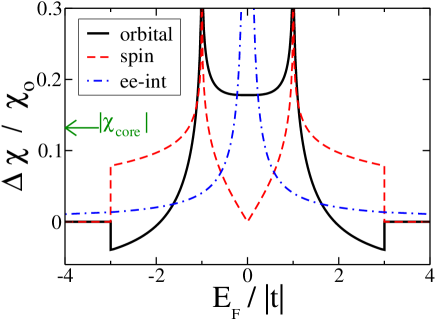
Figure 1: Continuous line: lattice contribution to the orbital magnetic susceptibility $(\Delta\chi_{orb})$ in units of $\chi_{o}=\mu_{o}\hbar^{-2}e^{2}|t|a^{2}$. Dashed line: Pauli’s spin paramagnetic contribution. Dashed-dotted line: orbital magnetic susceptibility from Coulomb electron-electron interactions (Eq. (6)). The arrow marks an estimate of the absolute value of the diamagnetic contribution from core electrons DiSalvo et al. (1979).

Now, we compare lattice’s OP with other contributions in the region $E_{F}\sim 0$, relevant for gate-doped graphene. Within our non-interacting model, the only remaining magnetic contribution is Pauli’s spin paramagnetism, given by $\chi_{spin}/\mu_{o}=2\mu_{B}^{2}\rho(E_{F})$ where $\mu_{B}$ is the Bohr magneton and $\rho(E_{F})$ is the density of states (per spin). This spin contribution is plotted in Fig. 1, where it is seen that it cannot compete with the dominant orbital contribution for low carrier densities $\rho_{e}$.

Core electrons, not considered in our $\text{pp}\pi$ band Hamiltonian, are another source of (dia)magnetic response. The estimate of Ref. DiSalvo et al. (1979), $\chi_{core}\sim-4.8\times 10^{-6}\text{emu/mol}$, translates into $\chi_{core}\sim-0.13\,\chi_{o}$, a value marked with an arrow in the scale of Fig. 1. Again, the orbital contribution for low $\rho_{e}$ is comparable or greater than this estimate of core diamagnetism.

Electron-electron interaction is the major ingredient left out in our model. Recently, its effect on the magnetic response has been calculated to first order within the Dirac cone approximation Principi et al. (2010). Two scenarios have been considered: Thomas-Fermi screened Coulomb interaction and contact (Hubbard-like) interaction, both leading to OP at finite doping. For the Coulomb case, the interaction’s contribution to the susceptibility can be written as Principi et al. (2010)

$$\chi_{ee}=\chi_{o}\frac{C}{E_{F}/|t|}\;,$$ (6)

with an interaction dependent constant $C\sim 0.04$, suitable for graphene over $\text{SiO}_{2}$. $\chi_{ee}$ is compared with the lattice contribution in Fig. 1. Graphene’s poor screening causes the divergence of $\chi_{ee}$ when $E_{F}\rightarrow 0$, making this contribution dominant. But even in this unfavorable case, the lattice contribution is not negligible. For instance, $\Delta\chi_{orb}\gtrsim\chi_{ee}$ for doping levels $n\!\gtrsim\!3.7\times 10^{13}\;\text{cm}^{-2}$, and for a typical doping $n\sim 4\times 10^{12}\;\text{cm}^{-2}$ one has $\chi_{ee}\sim 3\Delta\chi_{orb}$.

Finally, if (by some external means) screening were truly effective so that interactions could be described by a contact term $v_{o}$, Ref. Principi et al. (2010) provides the following expression for the interaction’s promoted orbital paramagnetism:

$$\chi_{ee}=g_{s}g_{v}\mu_{o}e^{2}\hbar^{-2}\frac{13}{256\pi^{2}}v_{o}\sim 0.027\;\chi_{o}\;\frac{U}{|t|},$$ (7)

where we have written the interaction as $v_{o}=UA_{c}/2$, with a Hubbard-like energy $U$, and area per unit cell $A_{c}=\tfrac{3\sqrt{3}a^{2}}{2}$. In order to compare this contribution with that of the lattice, we calculate the size of $U$ required for $\chi_{ee}$ of Eq. (7) to match the lattice contribution around $E_{F}\sim 0$. The answer turns out to be $U\sim 7|t|$, a value substantially larger than current estimates for graphene. This implies that, in any reasonable scenario of contact interactions, the lattice orbital contribution to paramagnetism would be the key player in the magnetic response of doped graphene.

Let us close with a remark on the effect of next-nearest neighbor hopping, temperature and disorder. As was already noted in Ref. Blinowski and Rigaux (1984), $t^{\prime}\approx 0.1t$ leads to a considerable electron-hole asymmetry in the magnetic response; the above qualitative discussion on the relevance of the several contributions, though, is not altered. Temperature and disorderKoshino and Ando (2007); *Nakamura broadens the diamagnetic delta-peak, such that lattice effects gradually lose relevance at a given temperature or disorder when the chemical potential decreases to zero.

Charge Response. The linear, static charge response of graphene is given by

$$\Pi(\bm{q})=\frac{1}{A}\!\!\!\sum_{\bm{k}_{1},s,s^{\prime}=\pm}\!\!\!f_{s\cdot s^{\prime}}(\bm{k}_{1},\bm{k}_{2})\frac{n_{F}(E^{s}(\bm{k}_{1}))-n_{F}(E^{s^{\prime}}(\bm{k}_{2}))}{E^{s}(\bm{k}_{1})-E^{s^{\prime}}(\bm{k}_{2})}\;,$$ (8)

with $\bm{k}_{1}=\bm{k}_{2}+\bm{q}$, and the prefactor $f_{\pm}$

$$f_{\pm}(\bm{k}_{1},\bm{k}_{2})=\frac{1}{2}\pm\frac{1}{2}\text{Re}\left(\frac{S(\bm{k}_{1})}{|S(\bm{k}_{1})|}\frac{S^{*}(\bm{k}_{2})}{|S(\bm{k}_{2})|}\right)\;.$$ (9)

Friedel oscillations are caused by intraband transitions ($+$-sign in Eq. (9)) with $q/2\sim k_{F}$, the Fermi wavevector (measured from the Dirac point). To understand graphene’s peculiarity, let us set $f_{+}=1$ in Eq. (8), and call the associated Lindhard-like response $\tilde{\Pi}$. Then, the dominant singularity in $\tilde{\Pi}$, corresponding to transitions across the Fermi surface, leads to the prototypical 2d square-root behavior

$$\tilde{\Pi}(q)\sim\frac{g_{s}g_{v}\sqrt{k_{F}}}{2\pi\hbar v}\sqrt{q-2k_{F}}\;\Theta(q-2k_{F}),$$ (10)

where $\Theta$ is Heaviside’s function and we have ignored any distortion of the isotropic Fermi surface around the two Dirac points. Within the Dirac cone approximation, the prefactor $f_{+}$ in Eq. (10) crucially vanishes for states on opposite sides of the Fermi surface. The physical interpretation is well known Cheianov and Fal’ko (2006): the involved states have opposite chirality and cannot be coupled by a perturbation diagonal in sublattice index. Nevertheless, this exact cancellation of $f_{+}$ holds true only in the scaling limit $k_{F}a\rightarrow 0$, and a finite value of $k_{F}a$ renders $f_{+}$ finite, something we generically label as lattice effect.

To see if this square root behavior is present also for the true prefactor $f_{+}$ as given in Eq. (8), we numerically analyze the response derivatives which we conveniently write as

$$\frac{\partial\Pi(\bm{q})}{\partial q_{\alpha}}=-\frac{g_{s}}{A2\pi}\text{Im}\int\!\!dE\,n_{F}(E)\sum_{\bm{k}}$$ (11)

$$\text{Tr}\{\hat{\cal G}_{\bm{k}}(E)\hat{\gamma}^{\alpha}_{\bm{k}}\hat{\cal G}_{\bm{k}}(E)(\hat{\cal G}_{\bm{k}-\bm{q}}(E)-\hat{\cal G}_{\bm{k}+\bm{q}}(E))\}\;.$$

We observe a clear anisotropy with a pronounced spike that hints at a singular behavior for the results in the y direction, absent in the x direction, where the behavior is closer to that of the (analytically known) Dirac cone approximation sup . The numerical results strongly suggest the restoration of a regular 2d response but with strong anisotropy. This is confirmed by the analytical treatment that follows.

Now we obtain analytically the charge response to lowest order in lattice effects. We start with the determination of the prefactor $f_{+}(\bm{q})$, that is, Eq. (9) for two states on opposite sides of the Fermi surface: $\bm{k}_{2}$ and $\bm{k}_{1}=\bm{k}_{2}+\bm{q}$, such that the vector $\bm{q}$ corresponds to the square-root singularity in the response. The latter condition requiring the $\bm{q}$-linked portions of the Fermi surface to be parallel. Upon a Jacobi-Anger expansion of the terms $\exp(i\bm{k}\cdot\bm{\delta}_{i})$, the structure factor can be written as $S(\bm{k})=3\sum_{n}J_{-1+3n}(k^{\prime}a)e^{i(-1+3n)\phi}$ where $J_{n}$ are Bessel functions of the first kind, and the separation from the Dirac point is $\bm{k}^{\prime}=\bm{k}-\bm{K}_{1}$, with polar coordinates $(k^{\prime},\phi)$. To lowest order in lattice effects, only $J_{-1}=-J_{1}$ and $J_{2}$ are to be retained. Then, the requirement $|S(\bm{k})|=\text{const}$ leads to the following expression for the Fermi surface in polar coordinates:

$$k^{\prime}_{F}(\phi)=k_{F}\left(1+\frac{k_{F}a}{4}\;\cos(3\phi)+{\cal O}(k_{F}a)^{2}\right),$$ (12)

where we have parametrized the Fermi energy by the would-be Fermi wave vector in the isotropic limit: $E_{F}=\hbar vk_{F}$.

To lowest order, the condition of parallel pieces of Fermi surface leads to the following relation between polar angles $(\phi_{1,2})$ of the involved ${\bm{k}}$-points: $\phi_{1}=\phi_{q}-\delta\phi$ and $\phi_{2}=\phi_{q}+\pi+\delta\phi$ with the lattice correction $\delta\phi=\frac{3}{4}\;(k_{F}a)\;\sin(3\phi_{q})$ and $\phi_{q}$ the polar angle of the joining vector $\bm{q}$ with modulus $q=2k_{F}(1+{\cal O}(k_{F}a)^{2})$. We can now write the phase of $S(\bm{k}^{\prime})$ as

$$\frac{S(\bm{k}^{\prime})}{|S(\bm{k}^{\prime})|}\sim-e^{-i(\phi+\theta)},$$ (13)

where $\phi$ is the polar angle of $\bm{k}^{\prime}$ and $\theta$ is the lattice correction to that phase given to lowest order by $\theta=\frac{1}{4}(k_{F}a)\;\sin(3\phi)$. This leads to the final expression for the prefactor

$$f_{+}(\bm{q})=\frac{(k_{F}a)^{2}}{8}(1-\cos(6\phi_{q}))+{\cal O}(k_{F}a)^{3}\;,$$ (14)

where $(2k_{F},\phi_{q})$ are the polar coordinates of $\bm{q}$ and which holds for both Dirac points. We note that the result of Eq. (14), although the lowest finite order in a $k_{F}$ expansion, already represents an excellent approximation for sizable Fermi levels well within the range of gate-voltage doped graphene’s samples sup .

Combining Eqs. (10) and (14), the dominant singularity of the true response is

$$\Pi\sim\frac{(k_{F}a)^{2}}{8}(1-\cos(6\phi_{q}))\frac{g_{s}g_{v}\sqrt{k_{F}}}{\pi\hbar v}\sqrt{q-2k_{F}}\;\Theta(q-2k_{F})\;.$$ (15)

We can now determine the density response associated to a local perturbing potential $V=u\delta(\bm{r})$ given by $\frac{\delta\rho(\bm{r})}{u}=\frac{1}{(2\pi)^{2}}\int d^{2}q\;e^{i\bm{q}\cdot\bm{r}}\Pi(\bm{q})$. The remaining integral is obtained from standard techniques Lighthill (1958), leading to the following asymptotic behavior for Friedel oscillations:

$$\frac{\delta\rho(\bm{r})}{\rho_{e}}=-\frac{(k_{F}a)^{2}}{2\sqrt{2}}(1-\cos(6\phi_{r}))\frac{u\rho_{e}}{E_{F}}\frac{\sin(2k_{F}r)}{(2k_{F}r)^{2}}\;.$$ (16)

While its $r^{-2}$ behavior is standard for a 2d system, its true origin as a lattice contribution to an otherwise null result (to order $r^{-2}$) is revealed by its amplitude, vanishing as $(k_{F}a)^{2}$ in the scaling limit $a\rightarrow 0$, and by its anisotropy reflecting the sixfold symmetry of the lattice.

Comparing Eq. (16) with the result coming from the Dirac cone approximation, Eq. (2), we first notice the phase shift of $\pi/2$. We further find for the crossover length between anomalous and regular Friedel oscillations $r_{c}\sim k_{F}^{-1}(k_{F}a)^{-2}$. For $k_{F}=1$nm^-1, we have $r_{c}\sim 100$nm which corresponds to an impurity concentration of $n_{i}\sim 10^{10}$cm^-2, recently found to be the intrinsic concentration of local impurities in graphene Ni et al. (2010). We thus expect Friedel oscillations to show anisotropic behavior and modify the RKKY-interactions for doping levels $E_{F}\lower 3.50006pt\hbox{$\stackrel{{\scriptstyle\textstyle>}}{{\textstyle\sim}}$}0.5$eV.

Summary. The simplest tight-binding model has been employed to study the lattice contribution to the magnetic susceptibility and (coarse-grained) charge response of doped graphene, for which the Dirac cone approximation produces a null result. The lattice magnetic response shows orbital paramagnetism for a wide range of filling factors, representing a relevant contribution when compared to other sources such as core diamagnetism, spin paramagnetism and electron-electron interaction induced orbital paramagnetism. Lattice effects restore the 2d regular behavior for the coarse-grained charge response, with Friedel oscillations decaying as $r^{-2}$ but with pronounced sixfold anisotropy, with maxima along bond’s directions. For clean samples with impurity concentrations of $n_{i}\sim 10^{10}$cm^-2 they become relevant for doping levels $E_{F}\lower 3.50006pt\hbox{$\stackrel{{\scriptstyle\textstyle>}}{{\textstyle\sim}}$}0.5$eV.

Acknowledgments. We are grateful to F. Guinea for useful discussions. This work has been supported by FCT under grant PTDC/FIS/101434/2008 and MIC under grant FIS2010-21883-C02-02.

References

- Novoselov et al. (2004) K. S. Novoselov et al., Science 306, 666 (2004).
- Geim (2009) A. K. Geim, Science 324, 1530 (2009).
- Neto et al. (2009) A. H. C. Neto et al., Rev. Mod. Phys. 81, 109 (2009).
- McClure (1956) J. W. McClure, Phys. Rev. 104, 666 (1956).
- Koshino et al. (2009) M. Koshino, Y. Arimura, and T. Ando, Phys. Rev. Lett. 102, 177203 (2009).
- Principi et al. (2009) A. Principi, M. Polini, and G. Vignale, Phys. Rev. B 80, 075418 (2009).
- Sepioni et al. (2010) M. Sepioni et al., Phys. Rev. Lett. 105, 207205 (2010).
- Fukuyama (1971) H. Fukuyama, Progr. Theor. Phys. 45, 704 (1971).
- Sharma et al. (1974) M. P. Sharma, L. G. Johnson, and J. W. McClure, Phys. Rev. B 9, 2467 (1974).
- Safran and DiSalvo (1979) S. A. Safran and F. J. DiSalvo, Phys. Rev. B 20, 4889 (1979).
- Blinowski and Rigaux (1984) J. Blinowski and C. Rigaux, J. Phys. (Paris) 45, 545 (1984).
- Cheianov and Fal’ko (2006) V. V. Cheianov and V. I. Fal’ko, Phys. Rev. Lett. 97, 226801 (2006).
- Wunsch et al. (2006) B. Wunsch et al., New J. Phys. 8, 318 (2006).
- Mariani et al. (2007) E. Mariani et al., Phys. Rev. B 76, 165402 (2007).
- Brey et al. (2007) L. Brey, H. A. Fertig, and S. Das Sarma, Phys. Rev. Lett. 99, 116802 (2007).
- Bena (2008) C. Bena, Phys. Rev. Lett. 100, 076601 (2008).
- Brihuega et al. (2008) I. Brihuega et al., Phys. Rev. Lett. 101, 206802 (2008).
- Stauber and Gómez-Santos (2010) T. Stauber and G. Gómez-Santos, Phys. Rev. B 82, 155412 (2010).
- (19) See supplementary material.
- Vignale (1991) G. Vignale, Phys. Rev. Lett. 67, 358 (1991).
- DiSalvo et al. (1979) F. J. DiSalvo et al., Phys. Rev. B 20, 4883 (1979).
- Principi et al. (2010) A. Principi et al., Phys. Rev. Lett. 104, 225503 (2010).
- Koshino and Ando (2007) M. Koshino and T. Ando, Phys. Rev. B 75, 235333 (2007).
- Nakamura (2007) M. Nakamura, Phys. Rev. B 76, 113301 (2007).
- Lighthill (1958) M. J. Lighthill, An Introduction to Fourier Analysis and Generalized Functions (Cambridge University Press, Cambridge, 1958).
- Ni et al. (2010) Z. H. Ni et al., Nano Lett. 10, 2868 (2010).