Rotated multifractal network generator

Abstract

The recently introduced multifractal network generator (MFNG), has been shown to provide a simple and flexible tool for creating random graphs with very diverse features. The MFNG is based on multifractal measures embedded in 2d, leading also to isolated nodes, whose number is relatively low for realistic cases, but may become dominant in the limiting case of infinitely large network sizes. Here we discuss the relation between this effect and the information dimension for the 1d projection of the link probability measure (LPM), and argue that the node isolation can be avoided by a simple transformation of the LPM based on rotation.

1 Introduction

The network approach for describing complex natural, social and technological phenomena has become very popular in the recent years. This can be accounted for the generality of its fundamental concept of representing the connections among the units (building blocks) of the system under study with a graph [1, 2]. Over the last decade it has turned out that networks corresponding to realistic systems can be highly non-trivial, characterised by a low average distance combined with a high average clustering coefficient [3], anomalous degree distributions [4, 5] and an intricate modular structure [6, 7, 8].

From the beginning of this new interdisciplinary field, network models have been playing a crucial role since they enable singling out the simplest aspects of complex structures and, thus, are extremely useful in understanding the underlying principles. Furthermore, models can also help testing hypotheses about measured data. In parallel with the discovery of the fine structure of real networks, many important and successful models have been introduced over the past 10 years for interpreting the different aspects of the studied systems. However, most of these models explain only a particular aspect of the network (clustering, a given degree distribution, etc.), and for each newly discovered feature a new model had to be constructed.

Due to this proliferation of network models, the concept of general network models and methods for generating graphs with desired properties has attracted great interest lately. A number of noteworthy methods have been proposed starting from the exponential random graph model [9, 10, 11, 12], through the hidden variable models [13, 14] (including the systematic study of the entropy of network ensembles [15]), the $dK$ series approach [16] and the use of $p$-adic randomised Parisi matrices [17, 18] to the Kronecker-graph approach [19, 20].

A very recently introduced approach along this line is the multifractal network generator (MFNG) [21], which was shown to be capable of generating a wide variety of network types with prescribed statistical properties, (e.g., with degree- or clustering coefficient distributions of various, very different forms). At the heart of this method lies a mapping between 2d measures defined on the unit square and random graphs. The main idea is to iterate a suitably chosen self similar multifractal (becoming singular in the limiting case) and enlarge the size of the generated graph (becoming infinite in the limiting case) in parallel. A very unique feature of this construction is that with the increasing system size the generated graphs become topologically more structured.

However, a slight drawback of the method is that when the size of the generated networks (and in parallel, the number of iterations in the multifractal) grow to infinity, isolated nodes overtake the majority of the graph in most settings, (see the SI of Ref.[21] for more details). Although this effect is usually not an issue when constructing graphs of sizes comparable to real networks, finding a way to circumvent it would still provide a noteworthy improvement, especially in the light of the non-trivial connections between convergent graph sequences in the infinite network size limit and 2d functions on the unit square [22, 23].

In this article we study the relation between the node isolation effect and the 1d projection of the link probability measure (LPM) used in the graph generation process. Furthermore, we propose a natural method to overcome the problem by a simple transformation based on rotation. The paper is organised as follows. In Sect.2. we overview the definition and most important properties of the multifractal network generator, while in Sect.3 we discuss the connection between node isolation and multifractality. We continue by proposing a modification of the original method avoiding the node isolation in Sect.4., which is tested in practise in Sect.5. Finally, we conclude in Sect.6.

2 The multifractal network generator

The multifractal network generator was inspired by earlier results from L. Lovász and co-workers proving that in the infinite network size limit, a dense graph’s adjacency matrix can be well represented by a continuous function $W(x,y)$ on the unit square [22, 23]. A similar approach was introduced by Bollobás et al. in Refs.[24, 25] and was used to obtain convergence and phase transition results for inhomogeneous random (including sparse) graphs. This two variable symmetric function (which can have a very simple form for a variety of interesting graphs, and was supposed to be either continuous or almost everywhere continuous) predicts the probability whether two nodes are connected or not.

In case of the MFNG the mentioned $W(x,y)$ is replaced by a self-similar multifractal [21]. We start by defining a generating measure on the unit square by dividing identically both the $x$ and $y$ axis to $m$ (not necessarily equal) intervals, splitting it to $m^{2}$ rectangles, and assigning a probability $p_{ij}$ to each rectangle ($i,j\in[1,m]$ denote the row and column indices). The probabilities are assumed to be normalised, $\sum p_{ij}=1$ and symmetric $p_{ij}=p_{ji}$. (Note that we normalize the probabilities of the generating measure instead of the integral of the latter because of the advantages of this choice to be discussed later.) Next, the LPM is obtained by recursively multiplying each rectangle with the generating measure $k$ times. This is in complete analogy with the standard process of generating a multifractal, resulting in $m^{2k}$ rectangles, each associated with a linking probability $p_{ij}(k)$ equivalent to a product of $k$ factors from the original generating $p_{ij}$ given as

$$p_{ij}(k)=\prod_{q=1}^{k}p_{i_{q}j_{q}}.$$ (1)

In our convention $k=1$ stands for the generating measure, thus, an LPM at $k=1$ is equivalent to the generating measure itself. The indices of the factors in (1) are given by

$$i_{q}=\left\lfloor\frac{(i-1)\prod_{r=1}^{q-1}\circ\,{\rm mod}\,m^{k-r}}{m^{k-q}}\right\rfloor+1,$$ (2)

where $\lfloor a/b\rfloor$ denotes the quotient (integer part) of $a/b$, the term $\prod_{r=1}^{q-1}\circ\,{\rm mod}\,m^{k-r}$ stands for subsequent calculation of the remainder after the division by $m^{k-r}$, and an analogous formula can be written for the indices $j_{q}$ as well. (For $q=1$, Eq.(2) simplifies to $i_{q}=\lfloor(i-1)/m^{k-1}\rfloor+1$). To obtain a network from the link probability measure, we distribute $N$ points independently, uniformly at random on the $[0,1]$ interval, and link each pair with a probability given by the $p_{ij}(k)$ at the given coordinates. (The above process is illustrated in Fig.1).

The diversity of the linking probabilities $p_{ij}(k)$ (and correspondingly, the structuredness of the generated graph) is increasing with the number of iterations, just like in case of a standard multifractal. When considering the “thermodynamic limit” of this construction ($k\rightarrow\infty$, $N\rightarrow\infty$) we would like to keep the generated networks sparse, i.e., ensure that the average degree of the nodes, $\left<d\right>$ remains constant. This can be achieved by an appropriate choice of the number of nodes as a function of $k$, using the following relation:

$$\left<d\right>=N(k)\sum_{i=1}^{m^{k}}\sum_{j=1}^{m^{k}}p_{ij}(k)a_{ij}(k),$$ (3)

where $a_{ij}(k)$ denotes the area of the box $i,j$ at iteration $k$. For simplicity, let us consider the special case of equal sized boxes $a_{ij}(k)=m^{-2k}$. Due to the normalisation of the linking probabilities in this case the above expression simplifies to $\left<d\right>=Nm^{-2k}$, thus, to keep the average degree constant when increasing the number of iterations for a given generating measure, the number of nodes have to be increased exponentially with $k$.

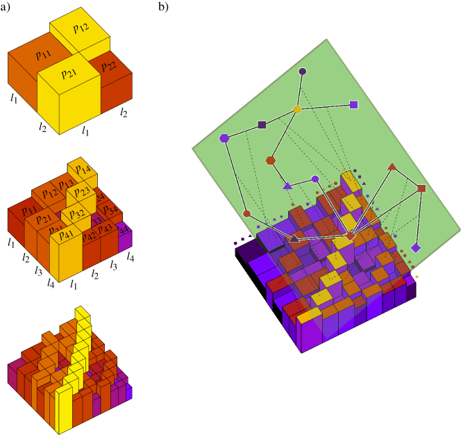
Figure 1: Schematic illustration of the multifractal graph generator. a) The construction of the link probability measure. We start from a symmetric generating measure on the unit square defined by a set of probabilities $p_{ij}=p_{ji}$ associated with $m\times m$ rectangles (shown on the left). The generating measure is iterated by recursively multiplying each box with the generating measure itself as shown in the centre and on the right. b) Drawing linking probabilities from the obtained LPM. We assign random coordinates in the unit interval to the nodes in the graph and link each node pair $I$, $J$ with a probability given by the probability measure at the corresponding coordinates, resulting in a graph drawn in the transparent green layer above the LPM.

The above construction could be made more general by replacing the “standard” multifractal with the $k$-th tensorial product of a symmetric 2d function $0\leq W(x,y)\leq 1$ defined on the unit square. Although the resulting $W_{k}(x_{1},...,x_{k},y_{1},...,y_{k})=W(x_{1},y_{1})\cdots W(x_{k},y_{k})$ function is $[0,1]^{2k}\rightarrow[0,1]$ instead of $[0,1]^{2}\rightarrow[0,1]$, with the help of a measure preserving bijection between $[0,1]$ and $[0,1]^{k}$ it could be used to generate random graphs in the same manner as with $p_{ij}(k)$.

At this point we also note that omitting the normalisation condition $\sum_{ij}p_{ij}=1$ for the generating measure gives the approach an additional flexibility which can come very handy in practical cases. Suppose that for a given setting of $k$, $N$ and the LPM we would like to increase the average degree in the obtained graph beside preserving the relative ratios of the linking probabilities (expected degrees) of nodes falling into the different rows of the LPM. A very natural idea in this case is to multiply each element in $p_{ij}(k)$ with the same factor $\eta>1$, and use the resulting matrix for generating a random graph in the same way. However, this multiplicative factor could be also introduced at the level of the generating measure instead, i.e., $\eta^{1/k}p_{ij}$ would also generate $\eta p_{ij}(k)$ for the LPM.

2.1 The degree distribution

An important property of the MFNG is that nodes with coordinates falling into the same row (column) of the LPM are statistically identical. This means that e.g., the expected degree or clustering coefficient of the nodes in a given row is the same. Consequently, the distributions related to the topology are composed of sub-distributions associated with the individual rows. The degree distribution can be expressed as

$$\rho^{(k)}(d)=\sum_{i=1}^{m^{k}}\rho_{i}^{(k)}(d)l_{i}(k),$$ (4)

where $\rho_{i}^{(k)}(d)$ denotes the sub-distribution of the nodes in row $i$, and $l_{i}(k)$ corresponds to the width of the row (giving the ratio of nodes in row $i$ compared to the number of total nodes). These $\rho_{i}^{(k)}$ take the form of [21]

$$\rho_{i}^{(k)}(d)=\frac{\left<d_{i}(k)\right>^{d}}{d!}e^{-\left<d_{i}(k)\right>},$$ (5)

where $\left<d_{i}(k)\right>$ denotes the average degree of nodes in row $i$. This is is given by $\left<d_{i}(k)\right>=N(k)p_{i}(k)$, where $p_{i}(k)$ corresponds to the linking probability in row $i$, given by

$$p_{i}(k)=\sum_{j}p_{ij}(k)l_{j}(k)$$ (6)

In more general, if the linking probability at iteration $k$ is described by $W_{k}(x,y)$, then the expected degree of a node having a position $x$ can be given as

$$\left<d(x)\right>=N(k)w_{k}(x),$$ (7)

where

$$w_{k}(x)\equiv\int dyW_{k}(x,y)$$ (8)

defines the 1d projection of $W_{k}(x,y)$ and is equivalent to the linking probability at position $x$. In case of the multifractal network generator this $w_{k}(x)$ has a simple step-wise constant form, showing a step-wise surface getting rougher and rougher with increasing $k$.

3 The isolated nodes and the multifractality of $w_{k}(x)$

According to Sect.2.1., the degree distribution and the fraction of isolated nodes depend on the projection of the link probability measure $p_{ij}(k)$ to the $x$ axis, (or equivalently, to the $y$ axis), given by $w_{k}(x)$. It is known that almost all projections of a multifractal such as $p_{ij}(k)$ with an information dimension larger than 1 to a 1d line result in measures with Euclidean support [26]. However, the projection to $w_{k}(x)$ is unfortunately a special case, belonging to the minority of projections yielding the “almost all” instead of “every” in the previous statement. As we shall see shortly, $w_{k}(x)$ is a multifractal itself with an information dimension smaller than 1, and this is the origin of the node isolation.

In Fig.2. we show $w_{k}(x)$ for $k=1$ and $k=2$ in a setting with equal sized boxes in the generating measure. For simplicity we shall assume equal sized boxes in the rest of this Section.

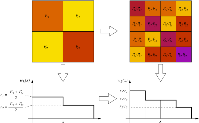
Figure 2: Projection of the LPM onto the edge of the unit square, resulting in a multifractal $w_{k}(x)$ function. For simplicity we assumed a 2 by 2 generating measure with equal box lengths.

Since the linking probability inside each box is constant, the shape of of $w_{k}(x)$ is step-wise, consisting of $m^{k}$ intervals (corresponding to the columns of the LPM), and the height of step $i$ is given by

$$r_{i}(k)\equiv\sum_{j=1}^{m^{k}}p_{ij}(k)l_{j}(k).$$ (9)

However, the multiplicative nature of the construction is inherited by $w_{k}(x)$ as well,

$$r_{i}(k)=\prod_{q=1}^{k}r_{i_{q}},$$ (10)

where

$$r_{i}\equiv\sum_{j=1}^{m}p_{ij}l_{j},$$ (11)

stand for the heights of the steps at the generating measure ($k=1$), and $i_{q}$ is given by (2). (This is demonstrated in Fig.2. for $k=2$). Thus, the evolution of $w_{k}(x)$ with $k$ is analogous to the standard construction of a multifractal embedded in the unit interval. Note however that if $\sum_{ij}p_{ij}=1$, then $w_{k}(x)$ is not normalised, e.g., for equal box lengths $\int w_{k}(x)dx=m^{-2k}$.

Multifractals are described by the $q$ ordered generalised fractal dimension $D(q)$ defined as follows (see e.g., Ref.[27]). Suppose that we divide the multifractal to boxes of size $\epsilon$, and the measure inside box $i$ is given by $p_{i}$. The function $\chi(q,\epsilon)$ is defined as

$$\chi(q,\epsilon)\equiv\sum_{i}p_{i}^{q}.$$ (12)

If $\epsilon$ is varied, $\chi(q,\epsilon)$ behaves as

$$\chi(q,\epsilon)\sim\epsilon^{D(q)(q-1)}.$$ (13)

Thus, $D(q)$ can be given as

$$D(q)=\lim_{\epsilon\rightarrow 0}\left[\frac{1}{q-1}\frac{\ln\sum_{i}p_{i}^{q}}{\ln\epsilon}\right].$$ (14)

In the special case of $q=1$ we have zero in the denominator, thus we take the $q\rightarrow 1$ limit and using l’Hospital’s rule we obtain

$$-\sum_{i}p_{i}\ln p_{i}\sim D_{1}\ln(1/\epsilon).$$ (15)

From the point of view of the degree distribution and the fraction of isolated nodes, the crucial $q$ value is $q=1$: When the number of iterations, $k\rightarrow\infty$, the fractal dimension of the support of the measure is given by $D(q=1)$. If it turns out that $D(q=1)<1$ for the $w_{k}(x)$ curve, then this means that the points giving the relevant contribution to the occurrence of links are concentrated on a fractal with a fractal dimension smaller than one, and thus, the majority of the nodes become isolated.

For a multifractal on the unit interval defined by a self-similar multiplication process such as in case of $w_{k}(x)$, (governed by Eqs.(9-11)), the $D(q)$ can be calculated analytically [27] as

$$D(q)=\frac{1}{(q-1)\ln(1/m)}\ln\left[\sum_{i=1}^{m}(r_{i}m)^{q}\right].$$ (16)

For $q=0$ the above expression yields $D(q=0)=1$, in agreement with the general picture of multifractals produced in a recursive multiplication process, where $D(q=0)$ equals the fractal dimension corresponding to a uniform generating object. For any multifractal in general, the $D(q)$ values monotonically decrease with increasing $q$. Thus, at $q=1$ in our case the $D(q)$ can reach $1$ only if $D(q)=1$ for any $q\in[0,1]$. According to (16), this can be achieved only if $r_{i}=1/m^{2}$ for all $i$. This means that unless the sum of probabilities in any row of the generating measure is the same, the $D(q=1)$ becomes smaller than 1, and the node isolation effect takes place.

4 Rotated measures

Our aim is to overcome the problem of the exact multifractality of $w_{k}(x)$ by modifying the construction in such a way that the projection of $W_{k}(x,y)$ determining the degree distribution has Euclidean support. Meanwhile, we want to keep the LPM a highly variable function so that very different distributions (leading to very different kinds of networks) could be still achieved. A simple idea is to rotate the LPM with a given angle $\alpha$ as shown in Fig.3., so that the direction of the projection determining the degree distribution no longer coincides with any of the special directions of the multifractal generation process. Thus, the construction of a random graph in this setting has the following main stages: we begin by generating a “standard” LPM for a chosen $k$, and “cut” a square rotated by an angle $\alpha$ from this measure as shown in Fig.3. Since the diagonal of this newly introduced square does not coincide with the diagonal of the original LPM, we have to symmetrise the measure inside the rotated square with respect to its diagonal. Finally, we distribute $N$ points uniformly at random along both sides of the rotated square and link each pair with a probability found at the given coordinates in the “rotated coordinate system”. (This last step is in complete analogy with the “standard” graph generation process).

Figure 3: A “standard” link-probability measure (oblique) with a rotated frame inside. The probabilities inside the rotated square have to be symmetrised along the diagonal. The linking probability of the green node can be calculated by summing up the probabilities “traversed” by the green line, each multiplied by the length of the intersection between the green line and the corresponding box. Due to the symmetry, this is equivalent to traversing first along the original line from the top until the diagonal is met, and then continue along the dashed line to the right.

When examining the behaviour of this construction with increasing $k$, the number of nodes used in the graph generation is adjusted according to the $\left<d\right>=$const. criterion, just as in case of the original settings. Due to the rotation and the symmetrisation, the polygons making up the link probability matrix are no longer arranged in a matrix like form, thus, (3) cannot be used straight away in this case. To calculate $\left<d\right>$ we need to first introduce a unique indexing over the polygons inside the rotated frame, and evaluate

$$\left<d\right>=N\sum_{i}p_{i}a_{i},$$ (17)

where $p_{i}$ and $a_{i}$ denote the probability and the area of the polygon $i$ (triangles, quadrangles and pentagons) defining the rotated link probability measure. The size of the various distances and the equations for the most important lines needed to evaluate (17) are given as a function of the rotation angle $\alpha$ in the Appendix.

The expected degree of a node at distance $h$ from the origin of the rotated square can be given by an expressions analogous to (7) as

$$\left<d(h)\right>=N(k)w_{k}(h),$$ (18)

where the linking probability $w_{k}(h)$ has to be calculated along a line parallel to the side of the rotated square. By denoting the set of polygons intersected by this line by $\Omega_{k}(h)$, we can express $w_{k}(h)$ as

$$w_{k}(h)=\sum_{j\in\Omega_{k}(h)}p_{j}\tilde{l}_{j}(h),$$ (19)

where $\tilde{l}_{j}$ denotes the relative length of the intersections divided by the length of the side of the rotated frame (see Fig.3). (These intersection lengths can be calculated with simple coordinate geometry, based on the equations given in the Appendix). Due to the symmetrisation of the rotated square, the boxes under the diagonal are rotated by $2\alpha$. Thus, in practise it is more simple to replace the summation (19) along a straight line by a summation along a broken line which is fully above the diagonal, as shown by the dashed green line in Fig.3.

The $w_{k}(h)$ function is the analogue of the $w_{k}(x)$ function for the rotated frame, and when $\alpha\rightarrow 0$, $w_{k}(h)\rightarrow w_{k}(x)$. As already noted in Sect.2, the 1d projection of the original link probability measure, $w_{k}(x)$, is always piecewise constant, where the constant intervals correspond to the columns of the link-probability measure. In case of $w_{k}(h)$ the situation is a bit more complex. In Fig.4. we depict two close by node positions in the rotated square. The lines along which one has to calculate the linking probabilities intersect with the same boxes. Furthermore, the lengths of the intersections are the same for the two lines in most of the boxes, except for the sections marked by red. Thus, the linking probability of the two nodes given by $w_{k}(h_{1})$ and $w_{k}(h_{2})$ will be quite close to each other as well, with the difference coming from the few different intersection lengths.

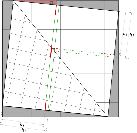
Figure 4: Two node positions in the rotated square, relatively close to each other shown by the green lines. They intersect with the same boxes, and in most cases the length of the intersections is the same as well. The different intersection lengths are marked by red.

Now let us imagine that we fix one of these two node positions, and set the corresponding linking probability $w_{k}(h)$ as a reference value. If we scan with the other node through a narrow interval of $h$ values such that the corresponding line still intersects with the same boxes, then due to the linear change in the intersection lengths, the change in $w_{k}(h)$ with respect to the reference value will be linear as well as a function of the $h$ difference between the two node positions.

From this it follows that if we scan through the total range of possible $h$ values, then the corresponding $w_{k}(h)$ curve of the linking probabilities will be piece wise linear. The break points between the linear segments correspond to the $h$ values where the line parallel to the rotated square boundary comes across a corner of the polygons defining the 2d link probability measure, and starts to intersect with a new polygon. Thus, to analytically calculate $w_{k}(h)$ we need to evaluate (19) only at the break points, and connect the results with linear segments. The $h$ value of the break points (corresponding to polygon corners) can be most easily calculated by changing the coordinate system to be aligned with the rotated square, having an origin at the top left corner. The details of this coordinate transformation are given in the Appendix. In Fig.5a we check the above for a 2 by 2 generating measure at $k=3$ by calculating $w_{k}(h)$ in both the break points and in two intermediate points between each adjacent break point pairs. Seemingly, the results for the intermediate points fall on the lines connecting the result for the break points.

The degree distribution can be obtained from $w_{k}(h)$ in three simple steps. The first step is the calculation of the distribution of the linking probability for the nodes, $\sigma^{(k)}(p)$. (By integrating $\sigma^{(k)}(p)$ as $\int_{p_{1}}^{p_{2}}\sigma^{(k)}(p)dp$ we receive the probability for a randomly chosen node to obtain a linking probability between $p_{1}$ and $p_{2}$, and the number of expected links on the node is given by the total number of nodes, $N$, multiplied by its linking probability). The $\sigma^{(k)}(p)$ can be calculated from $w_{k}(h)$ by a simple “projection” to the vertical axis as follows. Since we distribute the nodes uniformly at random along the side of the rotated square, the ratio of nodes falling into an interval of $[h_{1},h_{2}]$ is simply $(h_{2}-h_{1})/b$, where $b$ denotes the length of the side of the rotated square. Thus, a linear segment of $w_{k}(h)$, stretching from $h_{1}$ to $h_{2}$ contributes to $\sigma^{(k)}(p)$ with a “step” ranging from $p_{1}=w_{k}(h_{1})$ to $p_{2}=w_{k}(h_{2})$ with a height of $(h_{2}-h_{1})/(b|p_{2}-p_{1}|)$. (For an illustration see Fig.5b).

The second step in the calculation of the degree distribution is the transformation of $\sigma^{(k)}(p)$ into the distribution of the expected degrees for the nodes, $\tilde{\rho}^{(k)}(d)$. The difference between the degree distribution and $\tilde{\rho}^{(k)}(d)$ can be illustrated in the graph generation process: the expected degree of a node is simply its linking probability given by (19) multiplied by $N$, however, since the links are drawn randomly, its actual degree may become smaller or larger than that at the end of the link generation process. The $\tilde{\rho}^{(k)}(d)$ can be obtained from $\sigma^{(k)}(p)$ by a simple “stretching” in the horizontal direction, i.e., for any $p_{1}$ and $p_{2}$

$$\int_{p_{1}}^{p_{2}}\sigma^{(k)}(p)dp=\int_{x_{1}=Np_{1}}^{x_{2}=Np_{2}}\tilde{\rho}^{(k)}(x)dx,$$ (20)

where the integral on the right hand side corresponds to the probability for a randomly chosen node to have an expected degree falling between $d_{1}=Np_{1}$ and $d_{2}=Np_{2}$. We note that in case of the original settings without any rotation, both $\sigma^{(k)}(p)$ and $\tilde{\rho}^{(k)}(d)$ are given by trains of delta spikes with varying weights,

$$\sigma^{(k)}(p) = \sum_{i=1}^{m^{k}}l_{i}(k)\delta_{p,p_{i}(k)},$$ (21)

$${\tilde{\rho}}^{(k)}(d) = \sum_{i=1}^{m^{k}}l_{i}(k)\delta_{d,Np_{i}(k)},$$ (22)

where $p_{i}(k)$ denotes the linking probability in column $i$ of the original LPM given by (6). In contrast, for the rotated measures both $\sigma^{(k)}(p)$ and ${\tilde{\rho}}^{(k)}(d)$ take a step-wise form instead of delta spikes, (see e.g., Fig.5b).

The final step is to transform ${\tilde{\rho}}^{(k)}(d)$ into the degree distribution. Since the links are drawn independently of each other in both the original and the rotated settings, this can be achieved by taking the convolution of ${\tilde{\rho}}^{(k)}(d)$ with a Poisson-distribution as

$$\rho^{(k)}(d)=\int dx{\tilde{\rho}}^{(k)}(x)\frac{x^{d}}{d!}e^{-x}.$$ (23)

Figure 5: a) Checking the $w_{k}(h)$ of a 2 by 2 generating measure at $k=3$. The continuous line shows the piece wise linear linking probability as a function of $h$ obtained by connecting the values obtained at adjacent break points with straight lines. For each section we also calculated the linking probability in two intermediate points as well, the results are shown by the symbols. b) By projecting $w_{k}(h)$ to the vertical axis one obtains the distribution of the linking probabilities, $\sigma(p)$, which is step-wise. (Note that in order to emphasise the connection to $w_{k}(h)$, we have plotted $p$ on the vertical axis and $\sigma(p)$ on the horizontal axis). c) The distribution of the expected degrees, $\tilde{\rho}^{(k)}(d)$ is obtained by inflating $\sigma(p)$ according to the $\left<d\right>=Np$ relation. We have also plotted the corresponding degree distribution, $\rho^{(k)}(d)$, with dashed lines.

Based on the method detailed above, in the next Section we compare the evolution of the degree distribution with $k$ in the original settings and in the rotated scenario, (with a special focus on the ratio of the isolated nodes).

5 Applications

5.1 Degree distribution

For the comparison between the original settings and the rotated scenario we chose the 2 by 2 generating measure shown in Fig.6a. with a starting $N_{k=1}=30$, since the ratio of isolated nodes becomes significant quite fast without the rotation of the LPM in this case. The generating measure and $N_{k=1}$ fixed the average degree of the nodes to $\left<d\right>=7.5$. From $\left<d\right>$ we can calculate the number of nodes at the higher $k$ values in the original setting from (3). In case of the rotated scenario we use the same $\left<d\right>$, and calculate the number of nodes for any $k$ value from (17).

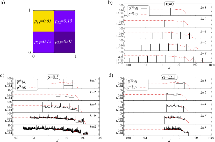
Figure 6: a) A 2 by 2 generating measure with equal box lengths. b) The distribution of the expected degrees, ${\tilde{\rho}}^{(k)}(d)$, (black, solid lines), and the degree distribution, $\rho^{(k)}(d)$, (red, dashed lines) in the original settings for $k=1,2,4,6,8$ on logarithmic scale. Since ${\tilde{\rho}}^{(k)}(d)$ corresponds to a delta-spike train according to (22), we used logarithmic binning for dealing with the singularities. c) The ${\tilde{\rho}}^{(k)}(d)$ (black, solid lines), and $\rho^{(k)}(d)$, (red, dashed lines) distributions at $k=1,2,4,6,8$ for a rotated frame at rotation angle $\alpha=0.5$ degrees. d) The ${\tilde{\rho}}^{(k)}(d)$ (black, solid lines), and $\rho^{(k)}(d)$, (red, dashed lines) distributions at $k=1,2,4,6,8$ for a rotated frame at rotation angle $\alpha=22.5$ degrees.

In Fig.6b we show the distribution of the expected degrees for the nodes, ${\tilde{\rho}}^{(k)}(d)$, on logarithmic scale for the original settings, obtained from (22), whereas Fig.6c-d show the same function for rotated frames at rotation angles $\alpha=0.5$ degrees and $\alpha=22.5$ degrees, respectively. We also plotted the corresponding degree distributions with dashed lines, however, the difference between the original and the rotated scenario is much more salient for ${\tilde{\rho}}^{(k)}(d)$. As explained in Sect.4., ${\tilde{\rho}}^{(k)}(d)$ consists of delta-spikes in case of the original settings (we have used binning in order to plot this singular function), and according to Fig.6b, as $k$ is increased, the distribution gets wider, and a significant part of it is shifted under $d=1$. This means that as we increase $k$, for larger and larger part of the nodes the expected degree becomes smaller than one, thus, the node isolation effect takes place. In contrast, Figs.6c-d show a different behaviour. Although the distributions become wider with increasing $k$ here as well, this tendency is much less pronounced compared to the $\alpha=0$ case. Furthermore, in case of Fig.6d the major part of the distribution stays above $d=1$ for the examined $k$ values.

In Fig.7a we show the ratio of isolated nodes as a function of the number of iterations. Due to the reduced spreading in the degree distribution with $k$ the rapid increasing tendency of $p(d=0)$ present in the original settings is modified to a very slowly increasing tendency for the rotated scenarios. The $p(d=0)$ at iteration $k=10$ is displayed in Fig.7b as a function of the rotation angle $\alpha$, showing an overall “U” shape with a minimum around 22.5 degrees. As pointed out previously, when $\alpha\rightarrow 0$, we recover the original settings of the MFNG. Although there seem to be many pairs of $\alpha$ values with very similar $p(d=0)$ values, we note that each $\alpha$ defines a different setting with unique attributes (e.g., the area of the rotated square affecting the average degree and the family of the $w_{k}(h)$ curves are always unique for each $\alpha$). The overall properties of a rotated setting (degree distribution, ratio of isolated nodes, etc.) change smoothly with the rotation angle for any $\alpha>0$. However, as argued in Sect.4. theoretically and shall be examined in Sect.5.2. numerically, the behaviour of the $D(q)$ curve does show a drastic change when switching from the $\alpha=0$ original setting to an $\alpha>0$ finite rotation angle. This change from a multifractal $D(q)$ to a non-multifractal one is not expected to be affected by any commensurability effect in rotation angles.

Figure 7: a) The ratio of isolated nodes as a function of the number of iterations for the examined generating measure (shown in Fig.6a). b) The ratio of isolated nodes at $k=10$ as a function of the rotation angle $\alpha$.

One of the big advantages of the original MFNG was that it provides a flexible tool for generating random graphs with realistic properties. Although examining to what extent this feature is affected by the rotation of the LPM is beyond the goals of this article, we present an example where power-law like degree distribution was achieved in the rotated scenario in the Appendix.

5.2 Measuring the $D(q)$ curve

The results shown in Sect.5.1. are very promising, since the rotation of the LPM drastically reduced the ratio of the isolated nodes in the studied example, especially in the case of larger rotation angles. However, an even more reassuring way for checking the effect of the modification of the MFNG is the measurement of the $D(q)$ curves corresponding to the $w_{k}(h)$ functions. As described in Sect.3., from the $D(q)$ at $q=1$ we can deduce the behaviour of the fraction of isolated nodes, i.e., if $D(q=1)=1$ in the $k\rightarrow\infty$ limit, than the isolated nodes cannot become dominant.

Before proceeding to the $D(q)$ curves, we have one important note. In practise we are always dealing with multifractals at a finite number of iterations, which have a lower size bound (lower length bound in our case) depending on the number of iterations. Below this lower size bound they are not any more structured and, thus, this size bound provides a lower bound for the size $\epsilon$ of the boxes with which we cover the multifractal when measuring $D(q)$ as described in Sect.3.

In case of the $w_{k}(x)$ of the original setting (without any rotation) this lower bound in $\epsilon$ is given simply by the width of the rows (columns). In case of the $w_{k}(h)$ of the rotated measure the situation is a bit more complex. First of all, when compared to the $w_{k}(x)$ of the original setting at the same number of iterations, $w_{k}(h)$ can contain much smaller segments. However, there are many adjacent segments with the same or almost the same slope of the linking probability, which can be united into single large segment, as shown in Fig.8.

Figure 8: A small part of the $w_{k}(h)$ of the rotated link probability measure at $k=8$, $\alpha=10.5$ degrees. The points correspond to the boundaries of the segments in which $w_{k}(h)$ is strictly linear. However, for many adjacent segments the slope is actually the same or nearly the same.

Thus, before the application of the $D(q)$ measuring procedure above, these segment joining were carried out, and the lower bound of $\epsilon$ was set to the average of the length of the resulting segments. This yielded still a much smaller value than in case of the original measure.

Interestingly, for the rotated frames when plotting $\ln\chi(q,\epsilon)$ as a function of $\ln\epsilon$, the curves seem to consist of two subsequent linear segments with different slopes. In contrast, the $\ln\chi(q,\epsilon)$ obtained from $w_{k}(x)$ in the rotation free settings shows a linear behaviour as a function of $\ln\epsilon$. The two types of $\chi(q,\epsilon)$ curves are shown in Fig.9.

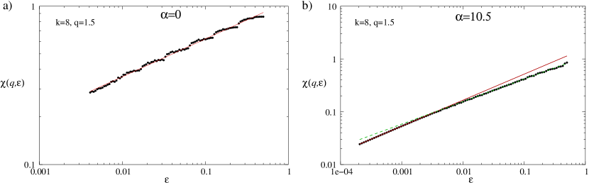
Figure 9: a) The $\chi(q,\epsilon)$ obtained for the $w_{k}(x)$ of the original setting at $k=8$ and $q=1.5$ on logarithmic scale (black symbols), together with a power-law fit (red line). b) The $\chi(q,\epsilon)$ of the $w_{k}(h)$ of the rotated frame at rotation angle $\alpha=10.5$ degrees with the same parameters $k=8$ and $q=1.5$ on logarithmic scale (black symbols). In contrast to the original settings, when fitting $\chi(q,\epsilon)$ with a power-law, the lower part and the upper part of the function yield different exponents, as shown by the continuous red line and the dashed green line respectively.

The $D(q)$ is obtained from the slope of these curves, which is straight forward in case of the $w_{k}(x)$ of the original settings. However, which part of the $\ln\chi(q,\epsilon)$ curve should we fit in case of the rotated measures? According to the definition given in (14) $D(q)$ should be evaluated in the $\epsilon\rightarrow 0$ limit, thus, we use the slope of the lower part of the $\ln\chi(q,\epsilon)$ curves in the rotated scenario for measuring $D(q)$.

In Fig.10. we show the results obtained for the $D(q)$ curves at various rotation angles. (For a comparison, the $D(q)$ curve of the original settings is shown as well).

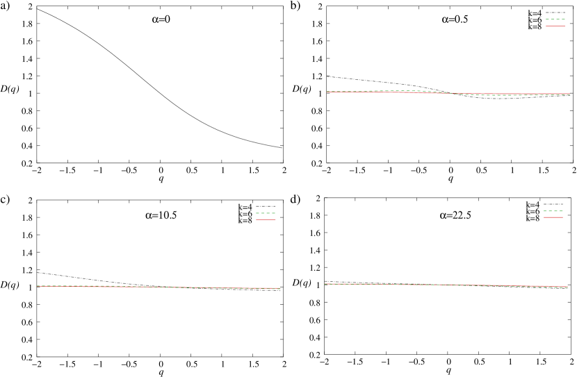
Figure 10: a) The $D(q)$ curve of the $w_{k}(x)$ function, corresponding to the original, “rotation-free” settings, obtained from (16). The $D(q)$ curves measured in the rotated scenario for $k=4,6,8$ at rotation angles $\alpha=0.5^{\circ}$, $\alpha=10.5^{\circ}$ and $\alpha=22.5^{\circ}$ are shown in panels b), c), and d), respectively.

From these figures it seems that $D(q)$ takes a trivial “non-multifractal” form at already $k=8$, and it is very close to 1 at $q=1$. The “precision” of the numerical $D(q)$ determination process at $q=1$ was tested on other 1d functions where we know that $D(q=1)=1$. According to that, for the rotated measures the numerically obtained $D(q=1)$ values are equal to $D(q=1)=1$ within error bound for $k=8$.

6 Summary

In summary, we investigated the node isolation effect of the MFNG from a new point of view. It had become clear that this phenomena is very closely related to the multifractality of the 1 dimensional projection of the LPM determining the degree distribution. According to general theorems concerning multifractals, the projection in question is a particular one, and in contrast, the vast majority of the other 1d projections of the LPM do not bear multifractal properties. Based on this observation we introduced a slight variation of the original MFNG method, involving the rotation of the LPM with a given angle. Due to the rotation, the projection determining the degree distribution is no longer a special projection in any aspects, thus, the node isolation effect is expected to disappear due to the lack of multifractality. The empirical studies support the theoretical reasoning above: the order $q$ generalised fractal dimension $D(q)$ in case of the projection of the LPM related to the degree distribution became trivial, and for the numerically accessible range of the number of iterations the fraction of isolated nodes showed a drastic reducement when compared to the original settings without any rotation.

Appendix

A1. Lengths

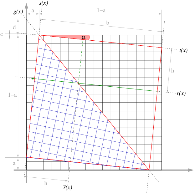
Figure 11: The geometry and the definition of the various lengths and sizes in the rotated link probability measure.

For the length of the interval $a$ in Fig.11 we can write

$$\frac{a}{1-a}=\tan\alpha,$$ (24)

thus,

$$a=\frac{\tan\alpha}{1+\tan\alpha}.$$ (25)

Similarly, we can write for $b$

$$\frac{a}{b}=\sin\alpha,$$ (26)

thus,

$$b=\frac{\tan\alpha}{\sin\alpha(1+\tan\alpha)}=\frac{1}{\cos\alpha+\sin\alpha}.$$ (27)

Furthermore,

$$c=a\tan\alpha=\frac{\tan^{2}\alpha}{1+\tan\alpha},$$ (28)

whereas

$$d=a\tan(\alpha+\pi/4)=a\frac{\sin(\alpha+\pi/4)}{\cos(\alpha+\pi/4)}=a\frac{\sin\alpha+\cos\alpha}{\cos\alpha-\sin\alpha}.$$ (29)

A2. Equations of the different lines

In the coordinate system shown in Fig.11. the equation of the top side of the rotated frame can be written as

$$t(x)=1+c-x\tan(\alpha).$$ (30)

Similarly, the equation of a parallel line below at a distance of $h$ is given by

$$r(x)=1+c-h\cos(\alpha)-h\sin(\alpha)\tan(\alpha)-x\tan(\alpha).$$ (31)

The equation of the diagonal can be expressed as

$$g(x)=1+d-x\tan(\alpha+\pi/4).$$ (32)

Finally, the equation of the left side of the rotated square is given by

$$s(x)=a+x\tan(\pi/2-\alpha),$$ (33)

and the equation of a parallel line shifted by $h$ to the right (corresponding to the dashed green line in Fig.11.) can be written as

$$\widehat{r}(x)=a+(x-h\cos\alpha-h\sin\alpha\tan\alpha)\tan(\pi/2-\alpha).$$ (34)

The equations given above can be used to calculate where a given line intersects with a given box boundary of the original link-probability measure, and from the location of the intersection points we can calculate the lengths/areas of the intersections between the lines and the boxes.

To calculate $\left<d\right>$ we have to calculate the area of each intersected box in the top triangular part of the rotated square. The boundary lines of this triangle can intersect with the boxes as summarised in Fig12.:

• in case the box intersects with only one line, then this divides it into either two trapezoids (Fig.12a), or into a triangle and a pentagon (Fig.12b),

• in case the box intersects with two lines, then there are still only three intersection points (instead of four), since the boundary lines must intersect each other on the boundary of the box. The remaining two unshared intersection points can take qualitatively three different positions: they can both fall on a side adjacent to the side of the shared intersection point (Fig.12c), they can both fall on the side opposite to the shared intersection point (Fig.12d), they can fall on two opposite sides adjacent to the side of the shared intersection (Fig.12e), or they can fall on two adjacent sides (Fig.12f).

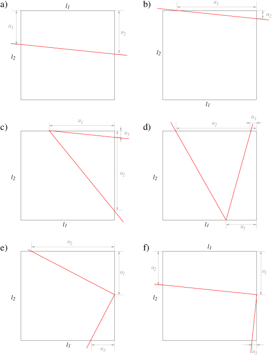
Figure 12: The six type of intersections of the boxes with the boundary lines of the top triangular part of the rotated square.

A3. Changing coordinate system

According to Fig.13., the new coordinates of a general point $x,y$ can be given as

$$\tilde{x} = \frac{x-a}{\cos(\alpha)}+(t(x)-y)\sin(\alpha),$$ (35)

$$\tilde{y} = (t(x)-y)\cos(\alpha),$$ (36)

where $t(x)$ denotes the equation of the topside of the rotated square in the standard coordinate system, given by (30).

Figure 13: Changing to the coordinate system of the rotated square.

A4. Generating skewed $\rho^{(k)}(d)$ in the rotated scenario

In Fig.14. we show an example where power-law like degree distribution is generated in the rotated scenario. According to the plots, a slight rotation preserves the degree distribution almost completely, whereas for larger rotations the skewed nature of $\rho^{(k)}(d)$ is slowly disappearing.

Figure 14: A power-law like degree distribution in the original settings at $k=4$ (black dot-dashed line), for which a slight rotation still preserves the skewed nature as shown by the solid red line corresponding to $\rho^{(k)}(d)$ at rotation angle $\alpha=0.002$ degrees. When $\alpha$ is increased, the skewedness of $\rho^{(k)}(d)$ is decreasing, as shown by the other two distributions corresponding to $\alpha=0.005$ and $\alpha=0.01$.

References

References

- [1] R. Albert and A.-L. Barabási. Statistical mechanics of complex networks. Rev. Mod. Phys., 74:47–97, 2002.
- [2] J. F. F. Mendes and S. N. Dorogovtsev. Evolution of Networks: From Biological Nets to the Internet and WWW. Oxford University Press, Oxford, 2003.
- [3] D. J. Watts and S. H. Strogatz. Collective dynamics of ’small-world’ networks. Nature, 393:440–442, 1998.
- [4] M. Faloutsos, P. Faloutsos, and C. Faloutsos. On power-law relationships of the internet topology. Comput. Commun. Rev., 29:251–262, 1999.
- [5] A.-L. Barabási and R. Albert. Emergence of scaling in random networks. Science, 286:509–512, 1999.
- [6] M. Girvan and M. E. J. Newman. Community structure in social and biological networks. Proc. Natl. Acad. Sci. USA, 99:7821–7826, 2002.
- [7] G. Palla, I. Derényi, I. Farkas, and T. Vicsek. Uncovering the overlapping community structure of complex networks in nature and society. Nature, 435:814–818, 2005.
- [8] S. Fortunato. Community detection in graphs. Physics Reports, 486:75–174, 2010.
- [9] O. Frank and D. Strauss. Markov graphs. Journal of the American Statistical Association, 81:832–842, 1986.
- [10] S. Wasserman and P. E. Pattison. Logit models and logistic regressions for social networks: I. an introduction, to markov graphs and p*. Psychometrika, 61:401–425, 1996.
- [11] G. Robins, T. Snijders, P. Wang, M. Handcock, and P. Pattison. Recent developments in exponential random graph (p*) models for social networks. Social Networks, 29:192–215, 2007.
- [12] J. Park and M. E. J. Newman. Solution of the two-star model of a network. Phys. Rev. E, 70:066146, 2004.
- [13] G. Caldarelli, A. Capocci, P. De Los Rios, and M. A. Muñoz. Scale-free networks from varying vertex intrinsic fitness. Phys. Rev. Lett., 89:258702, 2002.
- [14] M. Boguñá and R. Pastor-Satorras. Class of correlated random networks with hidden variables. Phys. Rev. E, 68:036112, 2003.
- [15] G. Bianconi. The entropy of randomized network ensembles. Europhys. Lett., 81:28005, 2008.
- [16] P. Mahadevan, D. Krioukov, K. Fall, and A. Vahdat. Systematic topology analysis and generation using degree correlations. ACM SIGCOMM Computer Communication Review, 36:135–146, 2006.
- [17] V. A. Avetisov, A. V. Chertovich, S. K. Nechaev, and O. A. Vasilyev. On scale-free and poly-scale behaviors of random hierarchical network. J. Stat. Mech., 2009:P07008, 2009.
- [18] V. A. Avetisov, S. K. Nechaev, and A. B. Shkarin. On the motifs distribution in random hierarchical networks. http://lanl.arxiv.org/abs/1005.3204, 2010.
- [19] J. Leskovec, D. Chakrabarti, J. Kleinberg, and C. Faloutsos. Realistic, mathematically tractable graph generation and evolution, using kronecker multiplication. In European Conference on Principles and Practice of Knowledge Discovery in Databases, pages 133–145, 2005.
- [20] J. Leskovec and C. Faloutsos. Scalable modeling of real graphs using kronecker multiplication. In Proceedings of the 24th International Conference on Machine Learning, pages 497–504, 2007.
- [21] G. Palla, L. Lovász, and T. Vicsek. Multifractal network generator. Proc. Natl. Acad. Sci. USA, 107:7640–7645, 2010.
- [22] L. Lovász and B. Szegedy. Limits of dense graph sequences. J. Comb. Theory B, 96:933–957, 2006.
- [23] C. Borgs, J. Chayes, L. Lovász, V. T. Sós, and K. Vesztergombi. Convergent sequences of dense graphs i: Subgraph frequencies, metric properties and testing. Advances in Math., 219:1801–1851, 2008.
- [24] B. Bollobás, S. Janson, and O. Riordan. The phase transition in inhomogeneous random graphs. Random Structures & Algorithms, 31:3–122, 2007.
- [25] B. Bollobás and O. Riordan. Random graphs and branching process. In B. Bollobás, R. Kozma, and D Miklós, editors, Handbook of Large-scale Random Networks, pages 15–115. Springer, Berlin, 2009.
- [26] K. Falconer. Fractal Geometry: Mathematical Foundations and Applications. John Wiley & Sons, Chichester, 2nd edition, 2003.
- [27] T. Vicsek. Fractal Growth Phenomena. World Scientific Publishing Co. Pte. Ltd., Singapore, 2nd edition, 1992.