Magnetohydrodynamic structure of a plasmoid in fast reconnection in low-beta plasmas

Abstract

Plasmoid structures in fast reconnection in low-beta plasmas are investigated by two-dimensional magnetohydrodynamic simulations. A high-resolution shock-capturing code enables us to explore a variety of shock structures: vertical slow shocks behind the plasmoid, another slow shocks in the outer-region, and the shock-reflection in the front side. The Kelvin-Helmholtz-like turbulence is also found inside the plasmoid. It is concluded that these shocks are rigorous features in reconnection in low-beta plasmas, where the reconnection jet speed or the upstream Alfvén speed exceeds the sound speed.

I Introduction

Magnetic reconnection Sweet (1958); Parker (1957); Petschek (1964) is a fundamental mechanism to power various events in laboratory, space, solar, and astrophysical plasmas. The reconnection process releases a fast plasma jet by consuming the magnetic energy stored in the upstream region. Such a plasma jet further interacts with the external environments and exhibits complex plasma phenomena. One of the most characteristic phenomena is a “plasmoid”, a magnetic island with plasmas embedded inside the magnetic loop. Plasmoids are well accepted to explain the satellite observation in the Earth’s magnetotail Hones (1977); Slavin et al. (1984, 2003) and morphological features in solar flare and coronal mass ejections Shibata et al. (1995); Lin et al. (2008); Linton & Moldwin (2009).

Motivated by the above and many other important reasons, the nonlinear evolution of magnetic reconnection and the associated plasmoid evolution has been studied over many decades. Significant insights have been obtained by magnetohydrodynamic (MHD) simulations in two Ugai & Tsuda (1977); Forbes & Priest (1983); Ugai (1986, 1987); Scholer (1989); Ugai (1992, 1995); Nitta et al. (2001); Abe & Hoshino (2001); Biskamp & Schwarz (2001); Tanuma & Shibata (2007); Bárta et al. (2008); Murphy (2010); Yu et al. (2011) and three dimensions Birn & Hones (1981); Hesse & Birn (1991); Ugai (1991); Ugai & Shimizu (1996); Ugai (2008). These simulations showed that the nonlinear evolution of the reconnection-plasmoid system involves complicated structures, such as slow shocks of the Petschek outflow Petschek (1964) and various shocks around the plasmoid Forbes & Priest (1983); Ugai (1987, 1995); Abe & Hoshino (2001).

Recently, reconnection research has been rapidly developing in relativistic astrophysics, too.Zenitani & Hoshino (2005); Watanabe & Yokoyama (2006); Zenitani et al. (2009, 2010) In this context Zenitani et al. (2010) carried out MHD simulations on relativistic magnetic reconnection. They discussed several shock structures that were not known in the nonrelativistic plasmoid physics: the postplasmoid vertical shocks and the shock-reflection structure in the plasmoid-front.

It is known that reconnection is highly influenced by upstream conditions. One key parameter is the Alfvén speed, which usually approximates the outflow jet speed. Another key parameter is the plasma beta, the ratio of the plasma pressure to the magnetic pressure. As will be discussed later, it corresponds to the ratio of the Alfvén velocity and the sound velocity. The beta is typically below the unity in the lower corona (Gary, 2001; Aschwanden, 2006) and the lobe (upstream region) of the magnetotail plasma sheet (Baumjohann et al., 1989).

In this paper, we explore fine structures of a plasmoid in fast reconnection when the upstream region consists of low-beta plasmas by using two-dimensional MHD simulations. Employing a high-resolution shock-capturing (HRSC) code, we successfully resolve a variety of shock structures. We confirm that the new shock structures in Ref. Zenitani et al., 2010 similarly appear in the nonrelativistic regime. We further discuss the condition for these shocks, and argue that they are common features of plasmoids in the low-beta plasmas. We also report some new features such as the Kelvin-Helmholtz-like turbulence inside the plasmoid and a potential signature of the corrugation instability of the slow shock surface.

This paper is organized as follows. We describe our numerical setup in Sec. II. We present simulation results and then investigate the local structures in depth in Sec. III. Section IV presents a brief parameter survey. We discuss these results in Sec. V, particularly focusing on the plasma beta condition. Section VI summarizes this paper.

II Numerical setup

We employ the following resistive MHD equations.

$$\frac{\partial\rho}{\partial t}+\nabla\cdot(\rho\bm{v})=0,$$ (1)

$$\frac{\partial\rho\bm{v}}{\partial t}+\nabla\cdot(\rho\bm{v}\bm{v}+p_{T}\bm{I}-\bm{B}\bm{B})=0,$$ (2)

$$\frac{\partial e}{\partial t}+\nabla\cdot\Big{(}(e+p_{T})\bm{v}-(\bm{v}\cdot\bm{B})\bm{B}+\eta\bm{j}\times\bm{B}\Big{)}=0,$$ (3)

$$\frac{\partial\bm{B}}{\partial t}+\nabla\cdot(\bm{v}\bm{B}-\bm{B}\bm{v})+\nabla\times(\eta\bm{j})=0,$$ (4)

where $p_{T}=p+B^{2}/2$ is the total pressure and $e=p/(\Gamma-1)+\rho v^{2}/2+B^{2}/2$ is the total energy density. The polytropic index is set to $\Gamma=5/3$. All other symbols have their standard meanings.

These equations are solved by a Godunov-type MHD code. Numerical fluxes are calculated by a Harten–Lax–van Leer (HLL) method.Harten et al. (1983) The spatial profiles are interpolated by a monotonized central (MC) limiter.van Leer (1977) The electric currents at the cell surfaces are calculated with the second order.Tóth et al. (2008) The second-order total variation diminishing (TVD) Runge–Kutta method is used for the time-marching.Shu & Osher (1988) The hyperbolic divergence cleaning method is employed for the solenoidal condition.Dedner et al. (2002)

The simulations are carried out in the $x$-$z$ two-dimensional plane. The reconnection point is set to the origin $(x,z)=(0,0)$. To reduce the computational cost, one quadrant ($x\geq 0,z\geq 0$) is solved considering the symmetry of the reconnection system. We set a symmetric boundary at $x=200$ and a conducting wall at $z=150$. The domain of $[0,200]\times[0,150]$ is resolved by $6000\times 4500$ grid cells. Harris sheet is employed as an initial model: $\bm{B}(z)=\tanh(z)\bm{\hat{x}}$, $\bm{v}=0$, $\rho(z)=1+\cosh^{-2}(z)/\beta_{up}$, $p(z)=0.5(\beta_{up}+\cosh^{-2}(z))$, where $\beta_{up}$ is the plasma beta in the upstream region. Importantly, we consider that the plasma beta is sufficiently lower than the unity, $\beta_{up}<1$. We set $\beta_{up}=0.2$ in our main run. By definition the Alfvén velocity in the upstream region is set to $c_{A,up}=|B|/\sqrt{\rho}=1$. Therefore the time is normalized by the Alfvén transit time of the Harris sheet thickness. Note that the evolution of reconnection is best characterized by the Alfvén transit time. The sound speed is uniform, $c_{s}=\sqrt{\Gamma\beta_{up}/2}\sim 0.408$.

It is known that the reconnection process is critically influenced by the resistivity $\eta$. In the MHD framework, a realistic fast reconnection requires a localized diffusion region in a vicinity of the reconnection pointPetschek (1964). This has been supported by simulations with spatially-localized resistivity.Ugai & Tsuda (1977); Scholer (1989); Biskamp & Schwarz (2001) Physically, such resistivity comes from local plasma instabilities, Hall effects,Birn et al. (2001) or electron kinetic effects,Hesse et al. (1999) none of which are fully understood. It is also known that physics-minded anomalous resistivity models allow fast reconnection. The resistivity is enhanced by a phenomenological measure of microphysics, e.g., the current intensity $(j/\rho)$. Since such quantity is the strongest around the X-point, the resistivity is localized and then Petschek-type fast reconnection spontaneously switches on.Ugai (1986, 1992) Regarding the macroscopic plasmoid dynamics, it was reported that both two models basically exhibit similar results.Ugai (1995) In this work, to keep the system simple and to see an evolution of a single reconnection, we employ the localized model,

$$\eta(x,z)=\eta_{0}+(\eta_{1}-\eta_{0})\cosh^{-2}(\sqrt{x^{2}+z^{2}}),$$ (5)

where $\eta_{1}=1/60$ is the localized resistivity and $\eta_{0}=1/1000$ is the background resistivity. A weak perturbation of $\delta A_{y}=-0.06\exp[-(x^{2}+z^{2})/4]$ is imposed to magnetic fields to speed up the reconnection onset.

III Results

The panels in Fig. 1 present the time development of $v_{x}$, which most significantly characterizes the system evolution. While we calculated the first quadrant ($z\geq 0$), the bottom half ($z<0$) is inserted to understand the structures better. The evolution can also be seen in the movie available online. The reconnection process starts around the origin. The localized resistivity causes magnetic field dissipation there, giving rise plasma inflow from the upstream region. Reconnection transfers the upstream magnetic fields toward the $+x$-direction along with an outflow jet. The flux transfer becomes faster and faster. Around $t\gtrsim 100$, the transfer rate $E_{y,R}=\eta_{1}j_{y,R}$ reaches its typical value of $0.05~{}[c_{A,up}B_{0}]$, where the subscript $R$ denotes the properties at the reconnection point. After that, the system exhibits a quasisteady evolution, whose reconnection speed remains fast, $E_{y,R}\sim 0.05$. Using properties at an upstream position $(x,z)=(0,5)$ (denoted by ^′), the rate can be re-normalized to $\mathcal{R}=E_{y,R}/(c^{\prime}_{A}B^{\prime})\sim 0.08$. This is a fast reconnection rate of $\mathcal{R}\sim\mathcal{O}(0.1)$.

Several characteristic structures already appear in Fig. 1a. The reconnection jet becomes Alfvénic ($v_{jet}\sim 1$) and there is a small magnetic island (plasmoid) in front of the jet. The plasmoid is heart-shapedSaito et al. (1995); Hirai et al. (2009), because MHD velocities are faster in the low-dense upstream region than ones in the plasma sheet ($z\sim 0$), and because dense plasmas throttle the outward motion of the plasmoid near the plasma sheet. One can recognize vertical structures of velocity jumps around $x\sim 21$ and $x\sim 48$ in the upstream plasmas. As the time goes on, the plasmoid grows bigger and bigger as it travels to the $+x$-direction. It seems that the macroscopic picture evolves self-similarly in later stages.Nitta et al. (2001) This is because the resistive spot and the Harris-sheet thickness become relatively smaller than the entire system, as the system grows larger. Meanwhile, fine structures become clear inside the plasmoid. Figure 1b shows the profile at $t=250$ of our main interest. The vertical jump structures are found around $x\sim 60$ and $x\sim 100$. The heart-shaped plasmoid now looks like a lobster-claw, as the bifurcated parts become much larger than ones in the earlier stage.

Shown in Fig. 2a is the plasma density $\rho$ and the flow pattern at $t=250$. Many plasmas are confined in the plasmoid. Some of the upstream plasmas are swept into the plasmoid by the reconnection jet. Other upstream plasmas directly enter the plasmoid across its outer boundary. In addition, the plasmoid eats Harris-sheet plasmas while it moves to the $+x$-direction. Figure 2b presents two thermodynamic properties. The upper half shows the temperature including the Boltzmann constant $T=p/\rho$. In general, plasmas are hot inside the reconnection jet and the plasmoid. The bottom half shows a useful measure $s=p/\rho^{\Gamma}$, which behaves similarly as specific entropy. Unless there is nonadiabatic heating, it is conserved throughout the convection $d/dt\big{(}{p}/{\rho^{\Gamma}}\big{)}=0$.

In the Secs. III.1-III.6, we take a closer look at local plasmoid structures at $t=250$, from the left Petschek outflow to the front side of the plasmoid. Note that boundary effects are completely ruled out. Since the fastest magnetosonic speed is $[c^{2}_{A,up}+c^{2}_{s}]^{1/2}\sim 1.08$, even the initial impact has not yet come back to the presented simulation domain.

III.1 Petschek outflow

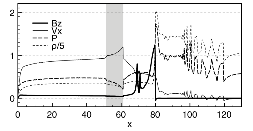
Figure 3: One dimensional cut of physical properties along the neutral line, $z=0$. The reconnected magnetic field $B_{z}$, outflow velocity $v_{x}$, plasma pressure $p$, and the density $\rho$. The shadow indicates the region between the vertical slow shock ($x=51.2$) and the fast shock ($x=61.2$).

As presented in Figs. 1 and 2a, the fast outflow jet flows from the reconnection point. The jet is separated from the upstream regions by slow shocks (Petschek, 1964), and therefore one can see hot and high-entropy plasmas inside the outflow channel (Fig. 2b). Figure 3 presents one-dimensional properties along the outflow line, $z=0$. The jet speed quickly increases to $\sim 0.8$-$0.9$, which is consistent with the Alfvén speeds in the upstream sides of the Petschek shocks. Note that the local Alfvén speeds are slightly slower than the initial speed of $1$, because the upstream conditions evolved. The jet speed increases again in the downstream ($x>51$), but we will discuss the downstream region later in Sec. III.3.

To examine the shock properties in depth, we carry out Rankine–Hugoniot analysis in various locations in the simulation domain at $t=250$. They are indicated by white marks in Fig. 1b and the relevant results are presented in Table 1. We determine the shock normal $\bm{\hat{n}}$ by the minimum variance analysis Sonnerup & Cahill (1967) and check the results by considering the magnetic coplanarity Colburn & Sonett (1966). We determine the shock velocity $v_{sh}$ by the mass conservation. Then, we compare the normal flow speed in the shock frame $(\bm{v}\cdot\bm{\hat{n}}-v_{sh})$ with the MHD wave speeds in the $\bm{\hat{n}}$-direction. We calculate Mach numbers with respect to the fast-mode, the Alfvén (intermediate) mode, and the slow-mode speeds: $\mathcal{M}_{f}$, $\mathcal{M}_{i}$, and $\mathcal{M}_{s}$. The subscript $1$ denotes the upstream properties and $2$ denotes the downstream properties. The first data (No. 1) in Table 1 correspond to the properties across the Petschek slow shock at $(x,z)\sim(40,\pm 1.35)$. The slope angle of the Petschek shock is small, ${\sim}0.03$. It is reasonable that the angle is a fraction of the field line slope in the upstream side ${\sim}0.095$ or the normalized reconnection rate $\mathcal{R}\sim 0.08$. The shock is stationary, $v_{sh}=0$, as expected. Across the shock, only the slow-mode Mach number changes supersonic to subsonic (Table 1). This is a reasonable indication of the slow shock.

Inside the outflow, we notice that there is a weak and narrow density cavity along the neutral line $z=0$, in the closer vicinity of the reconnection point. The small box inside Fig. 2a zooms up the relevant region. At $x=20$, the central density is $10\%$ lower than the surrounding density. This is because plasmas are hotter there, as pointed by a previous work Abe & Hoshino (2001). The central plasmas are Joule-heated near the reconnection point, while the surrounding plasmas are heated by the Petschek slow shocks. These two may be separated by contact discontinuities in an idealized limitHoshino et al. (2000); Abe & Hoshino (2001). Since our numerical scheme (HLL scheme) is weakly diffusive, the boundaries become unclear further downstream. In the real world, the contact discontinuities will disappear due to the field-aligned plasma mixing.

III.2 Postplasmoid slow shock

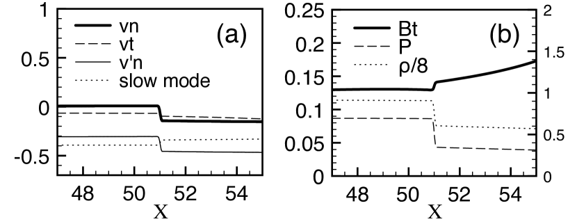
Figure 4: (a) One dimensional cut along $z=+6$. Normal velocity $v_{n}$ ($\approx v_{x}$), tangential velocity $v_{t}$, ($\approx v_{z}$), shock-frame normal velocity $v^{\prime}_{n}$, and the shock-frame slow-mode velocity in the $-x$-direction. (b) Tangential magnetic field $B_{t}$, pressure $p$, and density $\rho$. See the second vertical axis to measure $\rho$.

Behind the plasmoid one can see a sharp vertical structure at $x\sim 51$ in $v_{x}$ and $T$ (Figs. 1 and 2b). We find that this is a slow shock. We examine the shock properties near a typical point of $(x,z)\sim(51,6)$. The Rankine–Hugoniot properties are presented in No. 4 in Table 1. To better understand the structure, one-dimensional properties along $z=6$ is also presented in Fig. 4. Note that the shock normal is virtually parallel to the $x$-axis. The normal and tangential components are similar to the $x$ and $z$-components, respectively. In this case, the right side is the shock upstream, the left is the downstream, and the shock moves to the $+x$-direction at the speed of $v_{sh}\sim+0.31$. In Fig. 4a, the thin line shows the normal flow speed in the shock frame, $v^{\prime}_{n}=v_{n}-v_{sh}$. For comparison, the local-frame slow-mode speed in the normal direction is presented as the dotted line. Comparing them and the slow-mode Mach numbers $\mathcal{M}_{s}$ in Table 1, one can see that an upstream supersonic flow in the right side becomes subsonic in the left downstream. The shock exhibits many other slow-shock features. Along with the compression (Fig. 4b) and the adiabatic heating ($T$ in Fig. 2b), one can see that the tangential magnetic field $B_{t}$ ($\approx B_{z}+0.03$) decreases across the shock (Fig. 4b). Meanwhile, this is a nearly parallel shock and magnetic dissipation is quite limited. The measure $s$ is virtually unchanged (Fig. 2b) and the heating is weak ($T_{2}/T_{1}$ in Table 1).

As discussed in Ref. Zenitani et al., 2010, this vertical shock is related to a reverse plasma flow around the plasmoid. When the plasmoid moves to the right, it compresses plasmas in the nearby upstream region. Consequently, gas pressure drives plasma flows in the field-aligned directions. In addition, since there is a density cavity behind the plasmoid (Fig. 2a), the reverse flow in the postplasmoid region ($50<x<70$) is particularly strong, as can be seen in Fig. 1b ($v_{x}<0$; blue regions). The reconnection inflows usually move to the $\pm z$-directions, but they are accordingly modulated by the reverse flows (Fig. 2a). Due to the field-aligned expansion, the temperature becomes lower in the reverse flow region (Fig. 2b). The slow shock is located at the front, where the reverse flow supersonically hits the right-going shock front.

III.3 Postplasmoid outflow

We find that the postplasmoid vertical shocks affect the reconnection jet inside the outflow channel. The vertical shocks meet Petschek shocks at $x\sim 51.2$. In Fig. 3, one can see that the reconnection jet suddenly becomes faster around there. The jet further travels in the $+x$-direction, and then it hits the plasmoid at a shock at $x\sim 61.2$. The results of the shock analysis are shown in No. 3 in Table 1. This is a reverse-type fast shock Forbes & Priest (1983); Ugai (1987). The shadow in Fig. 3 indicates the outflow region between the vertical shock and the fast shock ($51.2<x<61.2$). It seems that the pressure gradient accelerates the jet in this shadow region. The jet speed reaches $v_{x}=1.2$ at the fast shock, which is much faster than the initial upstream Alfvén speed, $c_{A,up}=1$. A similar effect is reported by Shimizu & Ugai (2000, 2003), who claimed that deconfinement of the outflow channel leads to an adiabatic-type fluid acceleration.

We think that two mechanisms work in the shadow region. First, the system adjusts the balance condition of the Petschek shock, based on the upstream conditions. In the left quiet region ($x<51.2$), plasmas from the downstream side of the vertical shock come in to the Petschek shock. The outflow speed is well approximated by the upstream Alfvén velocity there. In the shadow region ($51.2<x$), plasmas from the upstream side of the vertical shock come in to the Petschek shock. The upstream Alfvén speeds are faster there, $c_{A,up^{\prime}}\sim 1.16$, mainly due to the lower density (Fig. 4b). Then, the Lorentz force at the Petschek shock accelerates plasmas to the “new” outflow speed of ${\sim}c_{A,up^{\prime}}$. One can see a rarefaction-like transition between the left Petschek flow and the right new Petschek flow in Fig. 3. Second, an adiabatic-type acceleration further boosts the jet.Shimizu & Ugai (2000, 2003) This is a simple hydrodynamic effect. Since the outflow speed exceeds the local sound speed of $c_{s}\sim 0.6$-$0.7$, such a supersonic flow is adiabatically accelerated when its cross section increases like a nozzle. It particularly works near the fast shock, where the plasmoid opens up the outflow channel,Shimizu & Ugai (2000, 2003) and so the final outflow speed of $\approx 1.2$ exceeds the maximum upstream Alfvén speed of $c_{A,up^{\prime}}\sim 1.16$.

According to the Rankine–Hugoniot analysis (No. 2 in Table 1), the Petschek shock in the postplasmoid region is stronger than the left-side (No. 1). The shocked plasmas are hotter and the entropy is higher than plasmas which come from the left Petschek shock, as seen in Fig. 2b. A sharp boundary separates plasmas from the left and right Petschek shocks. We think this boundary is a contact discontinuity, which originates from the shock-shock interaction point. Similarly, we expect that the field-aligned mixing will blur the discontinuity in the real world.

III.4 Outer shell and external slow shocks

The plasmoid is surrounded by a relatively sharp boundary. The Rankine–Hugoniot analysis across this outer shell (Nos. 5 and 6 in Table 1) tells us that it is a slow shock Ugai (1995). Judging from the heating ratio of $T_{2}/T_{1}$, the shock is stronger in the back side of the plasmoid than that in the front side, as discussed in previous literatureUgai (1995). In addition to the reconnection jet, the slow shock on the outer shell supplies hot plasmas into the plasmoid.

Outside the plasmoid, we find another pair of slow shocks around $(x,z)\sim(100,\pm 10)$. The Rankine–Hugoniot result is presented in No. 7 in Table 1. This shock is rather weaker than the other shocks. In fact, one can hardly find a jump in the measure $s$ in Fig. 2b, because dissipation is quite limited. However, our code does capture a clear jump structure in the velocity (Fig. 1b). Interestingly, as can be seen in Fig. 1a and the movie available online, the shock is originally located near the front edge. It gradually shifts backward to a stable location as the system evolves.

III.5 Internal structure

The reconnection jet hits the plasmoid at the fast shock (Sec. III.3), where plasmas enter the plasmoid. In the downstream side, there is a busy transition region at $x\sim 70$, where the shocked flow further slows down and accumulate the magnetic fields $B_{z}$ (Fig. 3). This region corresponds to the loop-top frontUgai (1987). Plasmas hit the loop-top front and then they diverge from the central region to the upper and lower regions inside the plasmoid. The reconnected fields are piled up between the loop-top front and the sharp tangential discontinuity (TD) at $x\sim 80$. The field $B_{z}$ is remarkably strong in the left side of the TD. The TD separates upstream-origin plasmas and plasmas initially located inside the Harris current sheet. This is visible in the $s$-profile in Fig. 2b. The entropy is high in upstream-origin plasmas, because they are shock-heated or Joule-heated. On the other hand, the right plasmas just come from the low-entropy Harris sheet.

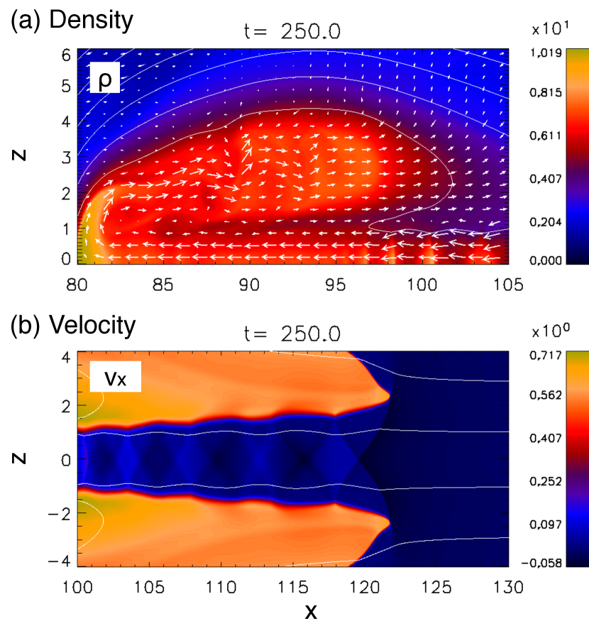
Figure 5: (Color online) (a) Plasma density $\rho$ inside the plasmoid at $t=250$. The white lines indicate magnetic field lines. The arrows indicate the plasma velocity in the moving frame of $v_{x}=+0.5$. The spatial length $2$ corresponds to $|v|=1$. (b) Profile of $v_{x}$ at $t=250$ in the front side. (Enhanced online)

Figure 5a presents the density profile inside the plasmoid. While the plasmoid is dynamically growing and expanding, the TD travels in the $+x$-direction at a nearly constant speed of $v_{T}\approx+0.5$. To understand the plasma motion better, the velocity profile in the moving frame of $v_{T}$ is shown by arrows. Plasmas at $z\sim 0$ constantly travels in the $-x$-direction from the right. After they hit the TD, they turn to the $+z$ direction, and then they are reflected to the $+x$-direction around $z\sim 2$. The TD works as a “magnetic wall” to reflect plasmas from the right side. In the original frame, this traveling wall hits the immobile Harris-sheet plasmas ($v\sim 0$). Therefore, the reflected flows are twice faster than the wall motion in Fig. 1b, $\sim 2v_{T}\sim 1$.

The fast reflected flow triggers velocity-shear-driven turbulence. In the online movie, one can see that a vortex rolls up where the flow turns its direction and that the reflected flow is deformed to a kink-type structure. We think this is due to the Kelvin-Helmholtz instability between the reflected jet and the surrounding medium. For example, typical parameters on the upper side of the reflected jet are $B\sim B_{0}/2\sim 0.5$, $\rho\sim\rho({t=0,z=0})\sim 6$, and $\Delta v\sim v_{T}\sim 0.5$, where $\Delta v$ is the velocity shear. From the linear theory,Miura & Pritchett (1982) we find that the shear is strong enough to bend the magnetic field lines, $\Delta v>2|B|/\sqrt{\rho}$, but is slower than the sonic upper limit, $\Delta v<2c_{s}$. Therefore, the shear layer would be unstable to the Kelvin-Helmholtz instability. One can see that the reflected flow is violently flapping in Fig. 1b and the online movie. The reflected flow and the resulting turbulence mix plasmas inside the plasmoid.

In Fig. 5a and the online movie, one can also see that the incoming flow repeatedly flaps in the right region of $98\lesssim x$ and $z\sim 0$. This is related to the shock-reflection structure which will be discussed in Sec. III.6.

III.6 Oblique-shock reflection

Shown in Fig. 5b is the $v_{x}$-profile in the front side of the plasmoid. The outer shells reach the leading edges of the plasmoid at $(x,z)\sim(121.8,\pm 2.4)$. Around the central region, there is immobile plasmas ($v\sim 0$), because high-density Harris-sheet plasmas are initially confined here. Outside the center, plasmas fast travel in the +$x$ direction. These twin flows are essentially driven by the reconnection outflow or the reflection by the magnetic wall. The central plasmas and the twin flows are separated by transition regions. The magnetic fields and plasmas flows are rather parallel to the transition regions, but they gradually enters from the central Harris sheet to the plasmoid flows.

As pointed out by Abe & Hoshino (2001), the transition region looks like an intermediate shock, across which the tangential magnetic fields change their polarities. Unfortunately, our Rankine–Hugoniot analysis fails to tell whether or not this is an intermediate shock (No. 8 in Table 1). This is probably due to the following three reasons. First, the assumption for the analysis may be invalid here. The Rankine–Hugoniot analysis deals with a time-stationary and one-dimensional structure. However, oblique shocks repeatedly hit the boundary regions as discussed later. A time-dependent flow and a weak curvature makes our analysis difficult. Second, the slow and intermediate speeds are hard to separate when the field lines are quasiperpendicular to the normal direction. Third, our numerical scheme (HLL scheme) is not ideal for the structure here. The HLL code excellently captures the fast shocks but handles other discontinuities in an upwind manner. When the characteristic speeds are slower than the fast-mode speeds by order of magnitude, the code smoothes the structure. Here, the fast speeds are typically $\sim 0.5$-$0.6$, while intermediate and slow speeds are on an order of $\sim{\mathcal{O}}(0.01)~{}[c_{A,up}]$. These three reasons make it difficult to discuss the slow/intermediate Mach numbers. In Table 1, we add asterisk signs to such unreliable Mach numbers. The third issue will be improved by a better scheme which fully considers intermediate discontinuities Miyoshi & Kusano (2005). In the right side near the flow edges (No. 9 in Table 1), the boundaries look like slow shocksSaito et al. (1995). Unfortunately, we fail to classify this shock for the same reasons. We expect that the intermediate shock changes to the slow shock through the switch-off shock Hau, L.-N.; Sonnerup, B. U. O. ; Hirai et al. (2009).

In the central channel, one can see that the oblique shocks propagate from the twin flow edges (Fig. 5b). They are fast shocks (No. 10 in Table 1). This is because the edges travel faster than the fastest right-going wave inside the central channel. These oblique shocks are repeatedly reflected by the intermediate shock regions Abe & Hoshino (2001). Such shock-reflection leads to a chain of the diamond-shaped patterns, as denoted by the “diamond-chain” structure in Ref. Zenitani et al., 2010. The second and third right ones look irregular in this case, but one can see that all other rectangles are excellently in order in Fig. 5b. The repeated shock-reflection explains a violent fluctuation in sonic properties in the front region ($95<x<120$) in Fig. 3.

Roughly speaking, the plasmoid edges travel at a sizable fraction of the reconnection jet speed $v_{jet}$, which is well approximated by the initial upstream Alfvén speed, $c_{A,up}$. On the other hand, since magnetic fields are very weak inside the current sheet, the right-going fast-mode speed is approximated by the sound speed in the current sheet. Therefore, a requirement for the oblique shock and the diamond-chain is

$${c_{s,cs}}<{c_{A,up}},$$ (6)

where the subscript $cs$ denotes the current sheet properties. Needless to say, our initial configuration satisfies this: $c_{s,cs}=c_{s}=0.408$ and $c_{A,up}=1$.

In the fronst side, there are small bow-shock-like structures around $x=121.8$, $z=2.55$–$2.75$, extending outward from the plasmoid edges. We do not recognize steep shocks there. We think they are the wave fronts of the fast mode Saito et al. (1995).

IV Beta Dependence

We carry out another two runs using different $\beta_{up}$ parameters, $\beta_{up}=0.1$ and $0.5$. All other parameters are the same as the main run. Figure 6a represents a snapshot with a lower upstream beta, $\beta_{up}=0.1$. The system builds up slower than the main run, because the system has relatively denser plasmas in the downstream Harris sheet. One can recognize many characteristic signatures except for the forward vertical slow shocks outside the plasmoid. Actually, there are slow shocks near $(x,z)\sim(82,\pm 9.8)$, but they are too small to recognize in the figure. The postplasmoid vertical shocks are located at $x\sim 40$. The velocity jump at the shock is smaller than the main run, because the sound speed is initially slower, $c_{s}=\sqrt{\Gamma\beta_{up}/2}\sim 0.29$.

Figure 6b shows the other run with $\beta_{up}=0.5$. One can see that the postplasmoid slow shocks are located in the back side of the plasmoid’s outer shell, $x\sim 55$. The other pair of slow shocks are located near the front edges of the plasmoid, $x\sim 115$. At a glance the front shocks look like switch-on fast shocks, but they are switch-off type slow shocks. Magnetic fields are gradually bent in the right side of the forward vertical slow shocks. Interestingly, a finger-like structure can be seen on the slow shock surface, around $2<|z|<6$ outside the plasmoid-front. It slowly grows there and it may eventually destroy and blur the forward slow shocks. We think that this is a signature of the corrugation instability of the slow shock surface Stone & Edelman (1995). However, detail analysis of the instability is beyond the scope of this paper.

V Discussion

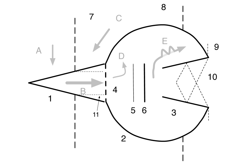
Figure 7: Schematic drawing of plasmoid structures: 1. Petschek slow shock Petschek (1964), 2. outer shell (slow shock)Ugai (1995), 3. intermediate shockAbe & Hoshino (2001) and slow shockSaito et al. (1995), 4. fast shock Forbes & Priest (1983); Ugai (1987), 5. loop-top front Ugai (1987), 6. tangential discontinuity, 7. postplasmoid vertical slow shock Zenitani et al. (2010), 8. forward vertical slow shock (Sec. III.4), 9. fast-mode wave front Saito et al. (1995), 10. shock-reflection (diamond-chain) Zenitani et al. (2010), 11. contact discontinuity (Sec. III.3), A. reconnection inflow, B. outflow jet, C. postplasmoid backward flow, D. internal flow, and E. flapping jet.

In this paper we visited many structures in and around the plasmoid. They are schematically illustrated in Fig. 7. This extends an informative result in an earlier work (i.e., Fig. 10 in Ref. Abe & Hoshino, 2001). Among these structures, the postplasmoid vertical shocks (Sec. III.2) and the shock-reflected diamond-chain structure in the front side (Sec. III.6) were recently found in the relativistic regime.Zenitani et al. (2010) We confirmed them in the nonrelativistic regime as well — they are ubiquitous, regardless of the relativistic effects. A reverse flow or a backward flow around the plasmoid is often found in recent large-scale simulationsAbe & Hoshino (2001); Zenitani et al. (2009), however, we clearly demonstrated that a slow shock stands at the front of the reverse flow. We also introduced another vertical slow shock outside the plasmoid. Those two vertical shocks are similarly found in other runs in our parameter survey.

We think that the vertical slow shocks are logical consequences of the low-beta condition of $\beta_{up}\lesssim 1$. From the following relation,

$$({c_{s,up}}/{c_{A,up}})^{2}=({\Gamma}/{2})\beta_{up},$$ (7)

we see $c_{s,up}<c_{A,up}$ when $\beta_{up}\lesssim 1$. As already discussed, the plasmoid-front propagates at a sizable fraction of the reconnection jet speed $v_{jet}\sim c_{A,up}$. When $\beta_{up}\lesssim 1$, the plasmoid supersonically travels in the system. At some location, the expanding plasmoid structure interacts with the surrounding plasmas at a supersonic speed, and then a shock stands there. Another interpretation is as follows. In a self-similarly expanding coordinate of the plasmoid system,Nitta et al. (2001) the surrounding plasmas supersonically flow in the $-x$-direction near the plasmoid-front, while the relative flow is very small near the reconnection point. A shock stands at the point where the supersonic flow slows down to subsonic speed. In summary, when $\beta_{up}\lesssim 1$, the plasmoid system will inevitably involve vertical slow shocks.

In addition, the compression effects by the plasmoid introduces another pair of vertical shocks outside the plasmoid. As discussed in Sec. III.2, the compression invokes the field-aligned flows in the ${\pm}x$ directions. In addition, the adiabatic heating or cooling weakly modify the local sound speed, $c_{s}=\sqrt{\Gamma s^{\frac{1}{\Gamma}}}\cdot p^{(\Gamma-1)/{2\Gamma}}\propto p^{{1}/{5}}$. In the main run, the relative velocity between the plasmoid system and the upstream plasmas are initially supersonic in the right side. It temporally becomes subsonic at the forward vertical shock $x\sim 100$ (Sec. III.4) due to the compression effects. However, due to the field-aligned acceleration in the $-x$-direction, the flow becomes supersonic again, and then it becomes subsonic at the postplasmoid vertical shock at $x\sim 51$ (Sec. III.2).

The positions of the vertical shocks depend on the $\beta_{up}$ parameter, because it controls the ratio of the sound speed to the Alfvénic plasmoid motion. When $\beta_{up}$ is lower than the main run ($\beta_{up}=0.1$), the expanding speed of the entire structure easily exceeds the sound speed. Therefore, the postplasmoid vertical shock is closer to the reconnection point, as demonstrated in Sec. IV (Fig. 6a). The forward vertical slow shock can be small, when the plasmoid compression effects are not strong enough to change the supersonic condition. Probably the forward vertical shock disappears in the extreme limit of $\beta_{up}\ll 1$. On the other hand, when $\beta_{up}$ is higher ($\beta_{up}=0.5$), the vertical slow shocks are nearer to the front-side of the plasmoid: the postplasmoid and forward ones are located just behind and in front of the plasmoid, respectively. As $\beta_{up}$ increases, the postplasmoid slow shock moves frontward even in the backward side of the plasmoid outer shell, and then it will eventually disappear. The forward slow shock will disappear when the Alvén speed is no longer supersonic, $\beta_{up}\sim 2/\Gamma=1.2$. Depending on $\beta_{up}(\lesssim 1)$, we expect one or two pairs of vertical slow shocks around the plasmoid.

Our discoveries can readily be applied to various numerical results in low-beta plasmas. Abe & Hoshino (2001); Tanuma & Shibata (2007); Zenitani et al. (2010); Yu et al. (2011) Abe & Hoshino (2001) carried out large-scale MHD simulation of a plasmoid in a similar configuration. While they did not mention it in the text, one can see a shock-like structure outside the plasmoid in RUN 2 with $\beta_{up}=0.25$ (the top panel in Fig. 9 in Ref. Abe & Hoshino, 2001). We think that this is a forward vertical slow shock. Zenitani et al. (2010) recognized a small shock outside the plasmoid (indicated by an arrow in Fig. 2c in Ref. Zenitani et al., 2010) in the relativistic regime with $\beta_{up}=0.1$. Inspired by this work, we carry out further analysis and confirm that it was a forward vertical slow shock. In multiple plasmoid systems, Tanuma & Shibata (2007) found “bow shocks” during the nonsteady reconnection under an anomalous-type resistivity with $\beta_{up}=0.2$ (Fig. 1d in Ref. Tanuma & Shibata, 2007). Judging from displacements, their plasmoid velocities are sub-Alfvénic, on an order of ${\sim}c_{s,up}<c_{A,up}$. In such a developing stage, the forward vertical shock is located near the front, and so it would be a forward slow shock. Finally, a recent work by Yu et al. (2011) reported a steepening structure of slow-mode wave behind the primary plasmoid (Fig. 15a in Ref. Yu et al., 2011). It would be related to a postplasmoid slow shock, as we found it in our relevant run with $\beta_{up}=0.5$ (Sec. IV; Fig. 6b).

The shock-reflection or the diamond-chain structure is also a characteristic in the low-beta condition. Dropping a factor of order unity, the requirement (Eq. 6) reads

$$\Big{(}\frac{c_{s,cs}}{c_{A,up}}\Big{)}\sim\Big{(}\frac{c_{s,cs}}{c_{s,up}}\Big{)}\sqrt{\beta_{up}}<1.$$ (8)

Although we still have a free parameter $({c_{s,cs}}/{c_{s,up}})$, the condition can be easily satisfied in the low-$\beta_{up}$ regimes.

Let us discuss some limitations of our simulation model. First, we assumed that the evolution in the bottom quadrant ($z<0$) is symmetric to that in the upper quadrant ($z>0$). We do not think the quadrant assumption affects the main shock structures, because Ref. Zenitani et al., 2010 was carried out without the assumption. On the other hand, we found the Kelvin-Helmholtz-like turbulence in the internal region (Sec. III.5). Since this class of instabilities may prefer odd-parity perturbation across the neural line ($z=0$), the central Harris sheet may flap in very late stages. This is left for future investigation. Second, in the three dimensions, it is known that quasiperpendicular slow shocks are unstable to the corrugation instability.Stone & Edelman (1995) We do see a potential signature of the instability even in the two dimensions (Sec. IV). In the real world, the vertical slow shocks may be violently folded and then we will see turbulent transition layers instead. Regarding the shock-reflected diamond-chain structure, the oblique fast shocks will be stableGardner & Kruskal (1964), but it is not clear how stable the intermediate shocks are. It is interesting to see how those structures are modulated in the three dimensions in future.

VI Summary

We carried out HRSC MHD simulations to study the fine structures of a plasmoid. We introduced new shock structures: (1) postplasmoid vertical slow shocks, (2) forward vertical slow shocks, and (3) shock-reflection structures, some of which were recently reported in Ref. Zenitani et al., 2010. We further found new features such as (4) the flapping motion of the reflected jet and (5) the finger-like instability of the slow shock surface. We interpreted that the vertical slow shocks and the shock-reflection are consequences of the Alfvénic plasmoid motion, which is supersonic in low-beta plasmas. We argue that these shocks are rigorous features of a reconnection system in low-beta plasmas.

Figure 1: (Color online) Time sequence of the velocity $v_{x}$, overlayed by the magnetic field lines. The two panels stand for (a) at $t=150$ and (b) at $t=250$. The white circles in the panel (b) indicates the locations where we analysized shock parameters (see also Table 1). (Enhanced online)

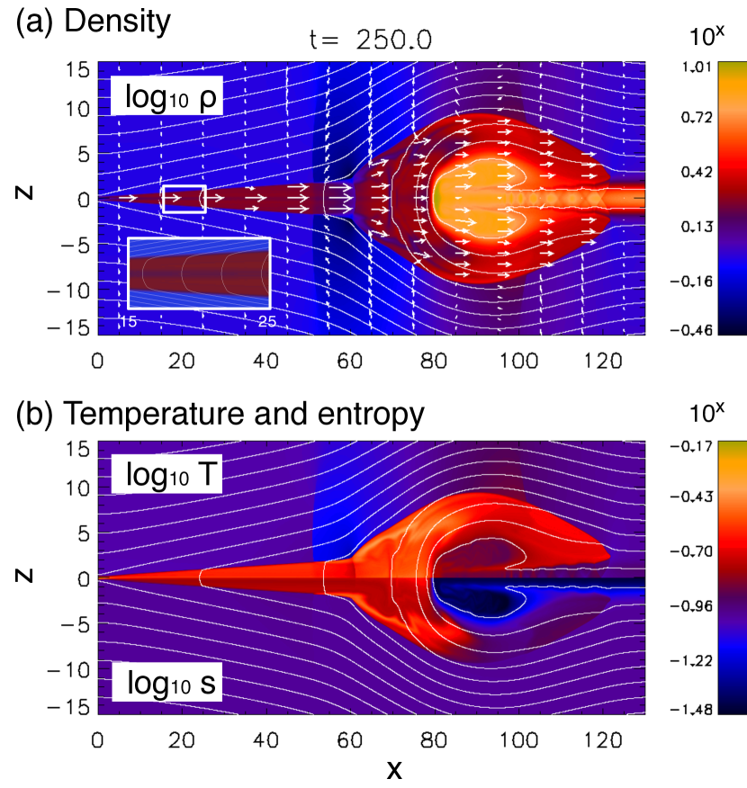
Figure 2: (Color online) Snapshots at $t=250$, overlayed by magnetic field lines. (a) Plasma density $\rho$. Arrows indicate plasma velocity: $|v|=1$ is projected to the length of $5$. The inner box shows the smaller doamin of $x\in[15,25]$ and $z\in[-1.5,1.5]$. (b) Plasma temperature $T$ in the upper half and the entropy measure $s=p/\rho^{\Gamma}$ in the bottom half.

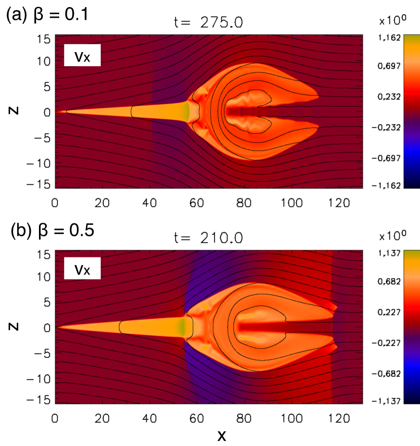
Figure 6: (Color online) The $v_{x}$-profiles in different simulation runs: (a) $\beta_{up}=0.1$, $t=275$ and (b) $\beta_{up}=0.5$, $t=210$.

#	Location	$(n_{x},n_{z})$	$v_{sh}$	$|\theta_{BN}|$	$\beta_{1}$	$\mathcal{M}_{f1}$	$\mathcal{M}_{i1}$	$\mathcal{M}_{s1}$	$\mathcal{M}_{f2}$	$\mathcal{M}_{i2}$	$\mathcal{M}_{s2}$	$T_{2}/T_{1}$
1	(40.0, 1.35)	(-0.03, 1.00)	0.0	86.3	0.22	0.06	0.98	2.49	0.04	0.69	0.69	2.72	(S) Petschek shock
2	(55.0, 1.75)	(-0.04, 1.00)	-0.013	86.3	0.098	0.06	0.88	3.22	0.04	0.58	0.58	4.58	(S) Petschek shock
3	(61.2, 0)	(-1.00, 0.00)	-0.40	90	303	1.41			0.77			1.38	(F) Reverse shock
4	(51.0, 6.0)	(1.00,-0.04)	0.31	9.4	0.12	0.41	0.42	1.34	0.33	0.34	0.78	1.33	(S) Postplasmoid vertical shock
5	(80.0, 8.4)	(-0.18, 0.98)	-0.06	86.5	0.16	0.05	0.85	2.47	0.03	0.56	0.65	2.54	(S) Outer shell
6	(110.0, 6.5)	(0.24, 0.97)	0.19	84.9	0.21	0.06	0.76	1.99	0.05	0.53	0.64	2.06	(S) Outer shell
7	(101.2, 10.0)	(0.94, 0.33)	0.54	25.2	0.23	0.43	0.49	1.15	0.39	0.44	0.87	1.15	(S) Forward vertical shock
8	(110.0, 1.5)	(-0.06,-1.00)	0.10	87.8	1.1	0.12	4.5*	6.5*	0.12	3.9*	4.0*	1.55	(U) Intermediate shock?
9	(120.0, 1.9)	(0.13,-0.99)	0.13	87.1	0.49	0.09	2.0*	3.8*	0.08	1.7*	1.9*	1.86	(U) Slow shock?
10	(120.9, 1.0)	(0.64,-0.77)	0.50	46.8	2.63	1.22	3.00	3.40	0.88	2.66	3.06	1.18	(F) Oblique shock

Table 1: Rankine–Hugoniot analysis. The subscripts $1$ and $2$ denote the upstream and downstream quantities. The locations $(x,z)$ in the simulation domain (see also Figure 1b), the shock normal vector $\bm{\hat{n}}$, the shock velocity $v_{sh}$, the angle between $\bm{\hat{n}}$ and the upstream magnetic field $\bm{B}_{1}$, the upstream plasma beta, flow Mach numbers to fast, intermediate (Alfvén), and slow-mode speeds, and the temperature ratio. The asterisk sign (*) indicates unreliable results (see Sec. III.6). The letter (S) indicates a slow shock, (F) is a fast shock, and (U) is unclassified.