On the Positive Mass, Penrose, and ZAS Inequalities in General Dimension

Abstract

After a detailed introduction including new examples, we give an exposition focusing on the Riemannian cases of the positive mass, Penrose, and ZAS inequalities of general relativity, in general dimension.

2000 Mathematics Subject Classification: 53C80, 53C24, 53C44.

Keywords and Phrases: General relativity, scalar curvature, black holes, minimal surfaces, zero area singularities, ZAS, positive mass inequality, Penrose inequality, ZAS inequality.

1 Dedication

It is an honor and a pleasure to contribute a paper to this volume celebrating Rick Schoen’s 60th birthday (which doesn’t seem possible since Rick is so much better at every sport than the author). Rick’s contribution to mathematics continues to be tremendous and is growing at an impressive rate, including his original research, collaborations with others, and the many students whom he has so expertly supervised. As successful as he has been for so many years, his continuing hard work and dedication reveals his genuine passion and love for mathematics. He is a role model for us all.

The ideas and directions discussed in this paper were in large part inspired by the positive mass inequality, proved in dimensions less than eight in Rick’s famous joint works with S.-T. Yau [37, 38, 36, 35]. The positive mass inequality is a beautiful geometric statement about scalar curvature which can equivalently be understood as the fundamental result in general relativity that positive energy densities in a spacetime imply that the total mass of the spacetime is also positive. In this paper we will discuss the Riemannian cases of the positive mass inequality, the Penrose inequality, and the ZAS (zero area singularity) inequality, describing how they are closely related in section 3. We apologize in advance for not making this a comprehensive survey of every interesting result in these areas, although we do recommend [26] as a very nice survey of the Penrose inequality. But first, in section 2 we begin with a mixture of well known facts and interesting new examples to motivate our later discussion.

2 Introduction

In this section we describe some of the ideas, motivations, and definitions that are central to general relativity, in general dimension. We also discuss intuition and include some new examples due to Lam [21, 22] of manifolds where the Riemannian positive mass inequality and the Riemannian Penrose inequality can be proved directly.

Broadly defined, general relativity encompasses any description of the universe as a smooth manifold with a Lorentzian metric, called a spacetime, of signature $(1,n)$, where usually $n=3$. Then the Einstein equation

$$G=(n-1)\omega_{n-1}T$$ (1)

can be taken to be the definition of the stress energy tensor $T$, where $\omega_{n-1}$ is the measure of the unit $(n-1)$ sphere. Thus, in dimension three, $G=8\pi T$. The Einstein curvature tensor $G=\mbox{Ric}-\frac{1}{2}R\cdot g$ has zero divergence by the second Bianchi identity. Furthermore, $T(\nu_{1},\nu_{2})$ is defined to be the amount of energy traveling in the unit direction $\nu_{1}$ as observed by someone going in the unit direction $\nu_{2}$. We comment that the Einstein equation can be derived from an action principle based on the Einstein-Hilbert action in the vacuum case, but we will take the Einstein equation as our starting point. The zero divergence property of $G$ (which is a consequence of the action principle) may be interpreted as a local conservation property for the stress energy tensor $T$.

2.1 The Schwarzschild Spacetimes

The vacuum case of general relativity is $G=0$ which, for $n\geq 2$, implies that $\mbox{Ric}=0$. Unlike Newtonian physics which is trivial in the vacuum case, general relativity is highly nontrivial in the vacuum case when $n\geq 3$. That is, there exist many solutions to $G=0$ other than the Minkowski spacetime metric

$$-dt\otimes dt+dx^{1}\otimes dx^{1}+...+dx^{n}\otimes dx^{n},$$ (2)

which include solutions describing gravitational waves which propagate at the speed of light. However, if we restrict our attention to spacetimes which are static and spatially spherically symmetric, then it is an exercise to show that for $n\geq 3$ there is precisely a one parameter family of vacuum solutions, called the Schwarzschild spacetimes. Explicitly, these spacetimes are

$$-\left(\frac{1-\frac{k}{r^{n-2}}}{1+\frac{k}{r^{n-2}}}\right)^{2}dt\otimes dt+\left(1+\frac{k}{r^{n-2}}\right)^{\frac{4}{n-2}}\left(dx^{1}\otimes dx^{1}+...+dx^{n}\otimes dx^{n}\right),$$ (3)

for $r>|k|^{1/(n-2)}$, where $r=\sqrt{(x^{1})^{2}+...+(x^{n})^{2}}$.

Note that $k=0$ corresponds to the flat Minkowski spacetime. Furthermore, it is an easy exercise to show that all of the $k>0$ spacetimes are scalings of each other, as are all of the $k<0$ spacetimes. Hence, up to scalings, equation 3 defines three special geometries, namely when $k=1,0,-1$. As we will see, each of these geometries inspires interesting physical statements.

For $k>0$, the spacetime in equation 3 represents the region outside a static black hole in vacuum. Note that there is a coordinate chart singularity at $r=k^{1/(n-2)}$ since the first metric term goes to zero. However, this value of $r$ is purely a coordinate chart singularity and not a true metric singularity. Kruskal coordinates [28] can be used to understand the entire Schwarzschild spacetime. The above choice of coordinate chart is limited in that it does not cover the interior region of the Schwarzschild spacetime which contains the true metric singularity, but it is ideal for our purposes as a way of visualizing the Schwarzschild spacetime as a perturbation of the Minkowski spacetime.

For $k<0$, the spacetime in equation 3 represents the region outside a static zero area singularity, called a ZAS [7]. Again, there is a singularity at $r=|k|^{1/(n-2)}$, but this time the singularity is a true metric singularity as the curvatures of the spacetime diverge to infinity as one approaches $r=|k|^{1/(n-2)}$. Note that while topologically the singularity is a coordinate $(n-1)$-sphere, the area of this sphere is zero. Hence, to an observer in the spacetime, the ZAS looks like a point singularity in this case.

Gravity, which is not a force in general relativity but instead is a perceived phenomenon, results from postulating that test particles in free fall follow geodesics. A curve in a spacetime with coordinates $\gamma(s)=(\gamma^{0}(s),\gamma^{1}(s),...,\gamma^{n}(s))$ is a geodesic if it satisfies the geodesic equation $\nabla_{\dot{\gamma}}\dot{\gamma}=0$, which in coordinates is

$$0=\ddot{\gamma}^{\alpha}(s)+\dot{\gamma}^{i}(s)\dot{\gamma}^{j}(s)\Gamma_{ij}^{\alpha}$$ (4)

for all $\alpha$, where we denote time as the zeroth coordinate and differentiation by $s$ with a dot. Hence, if we consider a curve with $\gamma(0)=(0,...,0,r)$ and $\dot{\gamma}(0)=(1,0,...,0)$ representing a test particle a distance $r$ away from the origin in the coordinate chart along the $n$th axis momentarily “at rest” going purely in the time direction, it follows from direct calculation that $\ddot{\gamma}(0)=(0,...,0,-a)$, where $a=\Gamma_{00}^{n}$ represents inward acceleration in the coordinate chart, and

$$\lim_{r\rightarrow\infty}ar^{n-1}=2k(n-2)$$ (5)

for the Schwarzschild spacetime. Hence, in the limit as $r$ goes to infinity, the geodesic accelerates in the coordinate chart towards the origin according to a $\frac{2k(n-2)}{r^{n-1}}$ inward acceleration law.

Now suppose we generalize Newtonian gravity to $n$ dimensions by defining the potential energy of a test particle divided by the mass of the test particle a distance $r$ from a point mass of mass $m$ to be $-\frac{Gm}{r^{n-2}}$ (where here $G$ is the universal gravitational constant). This corresponds to an inward acceleration law of $\frac{Gm(n-2)}{r^{n-1}}$. In the same way that setting the speed of light to one equates units of length and time, setting $G=1$ equates units of length to the power $n-2$ to mass.

In order to recover Newtonian dynamics from the Schwarzschild spacetime in the limit as $r$ goes to infinity, we set

$$\frac{2k(n-2)}{r^{n-1}}=\frac{Gm(n-2)}{r^{n-1}}$$ (6)

to derive $2k=Gm$. Thus, setting $G=1$ implies that $k=m/2$. Hence, when our one parameter family of Schwarzschild spacetimes is expressed as

$$-\left(\frac{1-\frac{m}{2r^{n-2}}}{1+\frac{m}{2r^{n-2}}}\right)^{2}dt\otimes dt+\left(1+\frac{m}{2r^{n-2}}\right)^{\frac{4}{n-2}}\left(dx^{1}\otimes dx^{1}+...+dx^{n}\otimes dx^{n}\right),$$ (7)

Newtonian dynamics is recovered by the behavior of nonrelativistic geodesics in the limit as $r$ goes to infinity, where $m$ is the total mass of the spacetime.

At first glance this result seems paradoxical since the Schwarzschild spacetimes are indeed vacuum solutions to the Einstein equation. How can they have nonzero total mass if they represent vacuum solutions? When $m>0$, the answer is that these spacetimes represent static black holes with event horizons at $r=(m/2)^{{1}/{(n-2)}}$ (“coincidentally” where the coordinate chart singularity is) which contribute a mass $m$ to the system. The more matter and gravitational waves that fall into a black hole, the most massive it becomes. Thus, while this is not precise, metaphorically one could think of the mass of a black hole as resulting from the mass and energy density that it has already consumed. Similarly, when $m<0$, it is reasonable to think of the ZAS singularity at the spatial origin as a singularity with negative mass. However, whereas the singularity of the Schwarzschild spacetime with $m>0$ is hidden inside the event horizon of a black hole, when $m<0$ the singularity of the ZAS is exposed for all observers to see. The time evolution of a ZAS has yet to be defined and it is not clear that it represents anything physical. However, geometrically ZAS are quite interesting and are very natural phenomena to study.

2.2 The Schwarzschild Metrics

We define the Schwarzschild metric to be the Riemannian manifold isometric to the $t=0$ hypersurface of the Schwarzschild spacetime. Explicitly, the Schwarzschild metric of mass $m$ in dimension $n\geq 3$ is

$$\left({\mathbb{R}}^{n}\backslash\bar{B},\left(1+\frac{m}{2r^{n-2}}\right)^{\frac{4}{n-2}}\left(dx^{1}\otimes dx^{1}+...+dx^{n}\otimes dx^{n}\right)\right),$$ (8)

where $\bar{B}$ is the closed ball of radius $\max(0,-m/2)^{1/(n-2)}$. Technically we have extended this Schwarzschild metric when $m>0$ since we are now allowing $r$ to go all the way down to zero. This is justified by the fact that for $m>0$, the above Riemannian metric is isometric to the $t=0$ slice of the Schwarzschild spacetime in Kruskal coordinates (which covers both exterior and both interior regions of the Schwarzschild spacetime) [28].

Again, all of the $m>0$ Schwarzschild metrics are scalings of each other, as are all of the $m<0$ Schwarzschild metrics. Hence, up to scalings, the Schwarzschild metrics define three important geometries to study, namely when $m/2=1,0,-1$. In particular, these three geometries are the cases of equality of the Riemannian Penrose inequality, the Riemannian positive mass inequality, and the Riemannian ZAS inequality (this last one modulo an open geometric conjecture), respectively, which we will discuss in detail later.

The conformal description of the Schwarzschild metrics given in equation 8 are a great way to gain some intuition about these metrics and, more generally, the notion of total mass. Recall that the parameter $m$ was chosen in our discussion of the Schwarzschild spacetime metrics to be physically compatible with our usual notion of total mass from Newtonian physics by looking at the accelerations of geodesics with respect to asymptotically flat coordinate charts. Even though the time dimension has been removed in the Schwarzschild metrics, the total mass $m$ is still present as the coefficient of the $\frac{1}{r^{n-2}}$ term in the expression of the metric. Hence, the total mass is directly related to the rate at which the Schwarzschild metric becomes flat at infinity.

Another important geometric characterization of the Schwarzschild metrics is that they are all of the spherically symmetric metrics which have zero scalar curvature. Hence, these metrics are important for understanding scalar curvature. As we will see later, scalar curvature is proportional to local energy density for zero second fundamental form slices of spacetimes. Hence, the fact that the Schwarzschild spacetime is vacuum implies that the Schwarzschild metric must have zero scalar curvature. This is also easily verified by direct calculation.

The Schwarzschild metrics of dimension $n$ have natural embeddings into flat spaces of dimension $n+1$, which is useful for another view of these geometries. When $m>0$, the $n$ dimensional Schwarzschild metric may be conveniently viewed as a spherically symmetric hypersurface of $n+1$ dimension Euclidean space (with the usual positive definite Euclidean metric) [6], as shown in figure 1 when $n=3$. Based on this, Greg Galloway noted that when $m<0$, one may do a Wick rotation where $w$ is replaced by $iw$ to conclude that for $m<0$, the $n$ dimensional Schwarzschild metric is isometric to a spherically symmetric hypersurface of $n+1$ dimension Lorentzian space, as shown in figure 2 when $n=3$.

These two figures are qualitatively correct in higher dimensions as well, although $R$ as a function of $w$ is not quite as explicit. Instead, we comment that for $m>0$, $\left(\frac{dR}{dw}\right)^{2}=\frac{R^{n-2}}{2m}-1$ gives the correct embedding in Euclidean space, and for $m<0$, $\left(\frac{dR}{dw}\right)^{2}=\frac{R^{n-2}}{2|m|}+1$ gives the correct embedding in Lorentzian space, for $n\geq 3$.

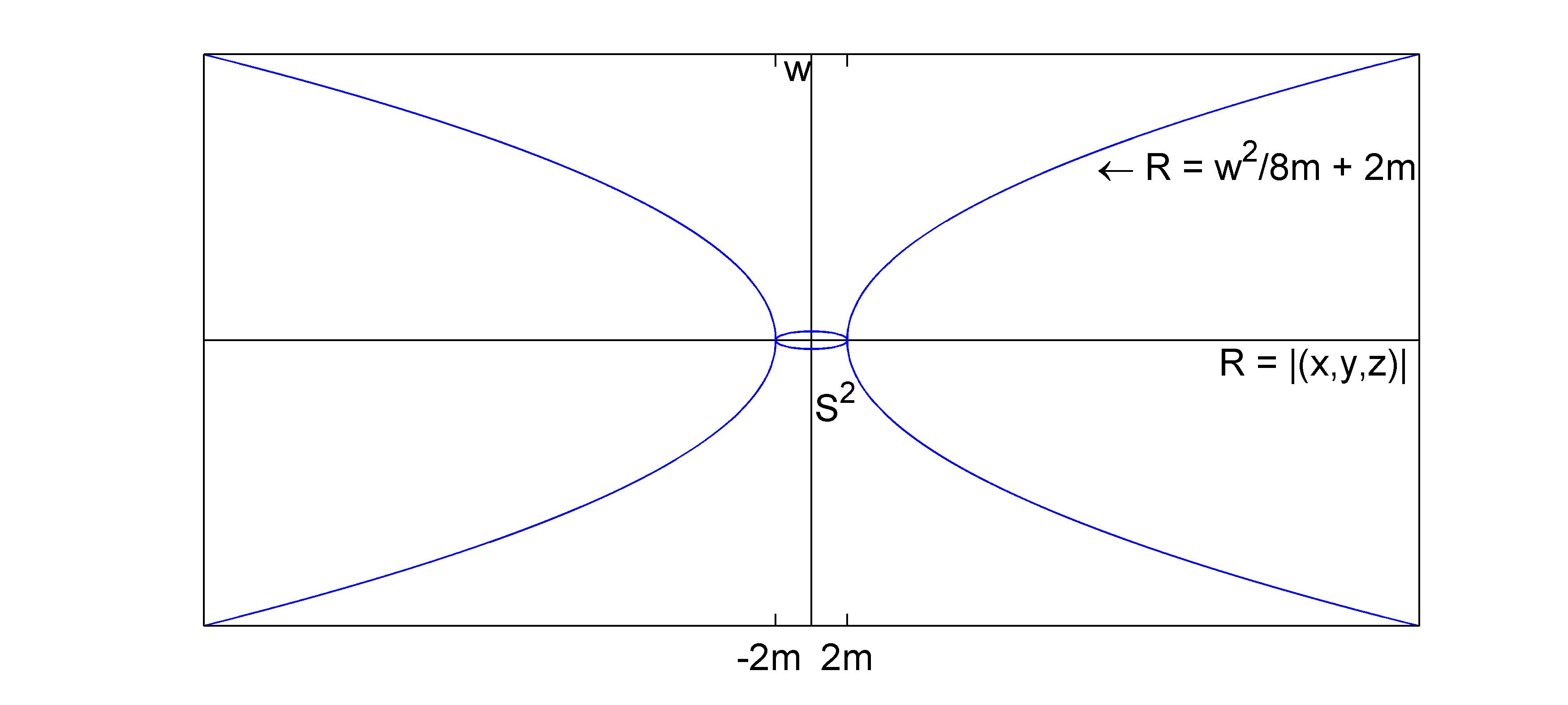
Figure 1: The three dimensional Schwarzschild metric of mass $m>0$ (in blue) viewed as a spherically symmetric submanifold of four dimensional Euclidean space {(x,y,z,w)} satisfying $R=w^{2}/8m+2m$, where $R=\sqrt{x^{2}+y^{2}+z^{2}}$.

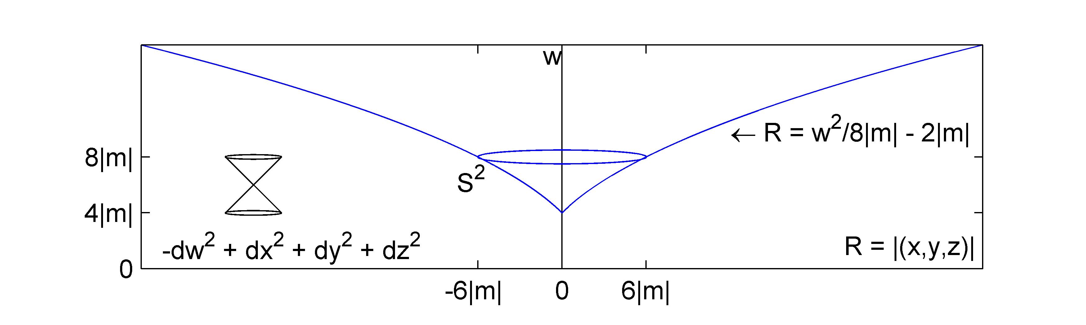
Figure 2: The three dimensional Schwarzschild metric of mass $m<0$ (in blue) viewed as a spherically symmetric submanifold of four dimensional Minkowski space {(x,y,z,w)} (with Lorentzian metric $-dw^{2}+dx^{2}+dy^{2}+dz^{2}$) satisfying $R=w^{2}/8|m|-2|m|$, where $R=\sqrt{x^{2}+y^{2}+z^{2}}$.

When $m>0$, figure 1 shows that the Schwarzschild metric also has a $Z_{2}$ symmetry by reflecting through the $w=0$ plane. The set of fixed points of this symmetry is a minimal $(n-1)$ sphere of $(n-1)$ volume $A=\omega_{n-1}(2m)^{\frac{n-1}{n-2}}$, where $\omega_{n-1}$ is the measure of the unit $(n-1)$ sphere. Going back to the conformal description of the Schwarzschild metrics in equation 8, this minimal sphere is realized at $r_{0}=(m/2)^{1/(n-2)}$. Furthermore, in the conformal picture, the $Z_{2}$ isometry is reflection through this sphere in the conformal coordinate chart, which explicitly is $r\rightarrow r_{0}^{2}/r$. Hence, zero goes to infinity and vice versa, highlighting the nonobvious fact that there is another asymptotically flat end in the neighborhood of $r=0$ in the conformal coordinate chart of equation 8.

When $m<0$, figure 2 gives a nice picture of the singularity. We comment that the nature of this singularity is complicated by the fact that the graph is becoming null at the singularity as well. We refer the reader to [7] for more discussion.

2.3 The Total Mass of Asymptotically Flat Manifolds

The Schwarzschild metrics give us examples of asymptotically flat manifolds where a notion of total mass is well defined. A logical next step is to find the most general notion of an asymptotically flat manifold for which a physically relevant definition of total mass can be defined. We refer the reader to papers by Bartnik who studied this problem in detail [2]. The most commonly used definitions for an asymptotically flat manifold $M^{n}$, $n\geq 3$, and its total mass $m$, are given below.

Definition 1.

[2] A complete Riemannian manifold $(M^{n},g)$ of dimension $n$ is said to be asymptotically flat if there is a compact subset $K\subset M$, such that $M\backslash K$ is diffeomorphic to $\mathbb{R}^{n}\backslash\{|x|\leq 1\}$, and a diffeomorphism $\Phi:M\backslash K\to\mathbb{R}^{n}\backslash\{|x|\leq 1\}$ such that, in the coordinate chart defined by $\Phi$, $g=g_{ij}(x)dx^{i}dx^{j}$, where

$$g_{ij}(x) =\delta_{ij}+O(|x|^{-p})$$

$$|x||g_{ij,k}(x)|+|x|^{2}|g_{ij,kl}(x)| =O(|x|^{-p})$$

$$|R(g)(x)| =O(|x|^{-q})$$

for some $q>n$ and $p>(n-2)/2$.

Definition 2.

[1, 2] The total mass $m$ of a complete, asymptotically flat manifold $(M,g)$ is defined to be

$$m=\lim_{r\to\infty}\frac{1}{2(n-1)\omega_{n-1}}\int_{S_{r}}\sum_{i,j}(g_{ij,i}-g_{ii,j})\nu_{j}dS_{r},$$ (9)

where $\omega_{n-1}$ is the volume of the $(n-1)$ unit sphere, $S_{r}$ is the coordinate sphere of radius $r$, $\nu$ is the outward unit normal to $S_{r}$ and $dS_{r}$ is the area element of $S_{r}$ in the coordinate chart.

The above definition for an asymptotically flat manifold is easily generalized to allow for more than one asymptotically flat end, where each connected component of $M\backslash K$, referred to as an end, is required to satisfy the stated asyptotically flat condition. For example, each Schwarzschild metric with $m>0$ has two asymptotically flat ends, as can be seen in figure 1. The definition of total mass then applies to each end separately, with each end having its own total mass.

The above definition for the total mass, also known as the ADM mass, was defined in [1]. (Definitions of total mass sometimes differ from the above by a factor, corresponding to different conventions than the one defined in section 2.1.) Later, Bartnik showed that the above definition is well-defined by showning that it is independent of the choice of asymptotically flat coordinates [2]. Finally, the above definition of total mass is compatible with our physically derived Schwarzschild metrics with metric components $g_{ij}=\left(1+m/2r^{n-2}\right)^{4/(n-2)}\delta_{ij}$, which is easily verified by direct calculation.

2.4 Local Energy Density and Scalar Curvature

Suppose that $(M^{n},g)$ is a Riemannian n-manifold isometrically embedded in an (n+1) dimensional Lorentzian spacetime. Suppose that $M^{n}$ has zero second fundamental form in the spacetime. This is a simplifying assumption which allows us to think of $(M^{n},g)$ as a “$t=0$” slice of the spacetime. Then by the Einstein equation (equation 1), the energy density $\mu$ as seen by an observer moving orthogonally to the hypersurface $M^{n}$ in the unit time direction $\nu$ is

$$\mu=T(\nu,\nu)=\frac{1}{(n-1)\omega_{n-1}}G(\nu,\nu)=\frac{R}{2(n-1)\omega_{n-1}},$$ (10)

where the last equality follows from the Gauss equation [28] and $R$ is the scalar curvature of $(M^{n},g)$.

Equation 10 reveals an important connection between energy density and scalar curvature, namely that they are the same, up to a factor, in the context of zero second fundamental form space-like hypersurfaces of spacetimes. This equation is the reason that the Riemannian positive mass inequality, the Riemannian Penrose inequality, and the Riemannian ZAS inequality, discussed in the next section, are not just important physical statements concerning energy density and total mass, but are also fundamental geometric statements about scalar curvature. More specifically, the physical assumption of nonnegative energy density everywhere implies that $(M^{n},g)$ must have nonnegative scalar curvature. Hence, the geometric study of asymptotically flat manifolds with nonnegative scalar curvature has physical implications.

2.5 Example: Conformally Flat Manifolds

Consider asymptotically flat manifolds of the form $({\mathbb{R}}^{n},g)$, $n\geq 3$, where

$$g=u(x)^{\frac{4}{n-2}}\delta,$$ (11)

where $\delta$ is the flat metric on ${\mathbb{R}}^{n}$ and $u(x)>0$ is $C^{2}$ and goes to one at infinity in a manner satisfying the asymptotically flat condition. Then direct computation shows that

$$R=-\frac{4(n-1)}{n-2}u(x)^{-\frac{n+2}{n-2}}\Delta u,$$ (12)

where $\Delta$ is the Laplacian operator of $({\mathbb{R}}^{n},\delta)$. (The exponent $\frac{4}{n-2}$ in equation 11 is chosen to make equation 12 particularly nice.) Hence, nonnegative energy density implies that our manifold must have nonnegative scalar curvature everywhere, which in turn implies that $u(x)$ must be superharmonic.

Also, $R=0$ in an open region $\Omega$ implies that $u(x)$ is harmonic in $\Omega$. Furthermore, the spherically symmetric harmonic functions in ${\mathbb{R}}^{n}$ are linear combinations of $1$ and $\frac{1}{r^{n-2}}$. Hence, if we require the asymptotically flat manifold to be spherically symmetric with zero scalar curvature outside a finite radius, then it follows that

$$u(x)=1+\frac{m}{2r^{n-2}}$$ (13)

there, for some $m$. Hence, the manifold will be isometric to a Schwarzschild metric outside the finite radius. This is a convenient assumption to make since then the total mass is just $m$. Then

$$m = \lim_{r\rightarrow\infty}\frac{2}{(n-2)\omega_{n-1}}\int_{S_{r}}-\langle\nabla u,\nu\rangle dS_{r}$$ (14)

$$= \frac{2}{(n-2)\omega_{n-1}}\int_{M^{n}}-\Delta u\;dV_{\delta}$$ (15)

$$= \frac{2}{(n-2)\omega_{n-1}}\int_{M^{n}}\frac{n-2}{4(n-1)}Ru(x)^{\frac{n+2}{n-2}}\;dV_{\delta}$$ (16)

$$= \int_{M^{n}}\frac{R}{2(n-1)\omega_{n-1}}u(x)^{\frac{2-n}{n-2}}\;dV_{g}$$ (17)

where $\nu$ is the outward unit normal to $S_{r}$, $dS_{r}$ is the area form of $S_{r}$, $dV_{\delta}$ is the volume form of $(M^{n},\delta)$, and $dV_{g}$ is the volume form of $(M^{n},g)$. The first equality follows from the special form of $u(x)$ given by equation 13, although not surprisingly it is true for all conformally flat asymptotically flat manifolds. The second equality is the divergence theorem. The third step follows from equation 12 and the fourth step follows from $dV_{g}=u(x)^{\frac{2n}{n-2}}dV_{\delta}$.

Now suppose that we let $u(x)=1+\epsilon v(x)$, where $v(x)$ is $C^{2}$, superharmonic, and equal to $\frac{1}{2r^{n-2}}$ outside a finite radius. Then in the limit as $\epsilon$ goes to zero, $u(x)\approx 1$ and

$$m\approx\int_{M^{n}}\frac{R}{2(n-1)\omega_{n-1}}\;dV_{g},$$ (18)

by which we mean that the ratio of the left hand side to the right hand side of this equation equals one in the limit as $\epsilon$ goes to zero.

Hence, equation 18 implies that the total mass is approximately the integral of energy density (as defined in equation 10) in this example. This is what one would expect from Newtonian physics. Equivalently, if we take this model to be the physically relevant perturbation of Minkowski space and its flat ${\mathbb{R}}^{3}$ zero second fundamental form hypersurface corresponding to the Newtonian limit (a discussion which we will skip), this argument defines the correct proportionality constant in the Einstein equation (equation 1).

However, especially as we get further from the $\epsilon=0$ limit, it is important to note that total mass is not the integral of energy density. Since $u(x)$ is superharmonic, the maximum principle implies that $u(x)\geq 1$. Hence, in this particular example,

$$m\leq\int_{M^{n}}\frac{R}{2(n-1)\omega_{n-1}}\;dV_{g},$$ (19)

which roughly corresponds to the fact that Newtonian potential energy, which for two positive point masses is $-m_{1}m_{2}/r^{n-2}$, is negative. However, there are also examples of asymptotically flat manifolds where

$$m\geq\int_{M^{n}}\frac{R}{2(n-1)\omega_{n-1}}\;dV_{g}.$$ (20)

If fact, given any asymptotically flat manifold with nonnegative scalar curvature, one can multiply it by a conformal factor to achieve zero scalar curvature everywhere. By the Riemannian positive mass inequality (which currently requires $n\leq 7$ or $M^{n}$ to be spin) discussed in the next section, the total mass of the resulting zero scalar curvature manifold will be positive, unless the resulting manifold is the flat metric on ${\mathbb{R}}^{n}$. Hence, the connection between local energy density and total mass is highly nontrivial.

The Riemannian positive mass inequality simply states that nonnegative energy densities should imply that the total mass is also nonnegative, with zero total mass only for the flat metric on ${\mathbb{R}}^{3}$. Physically, if this were not the case, then the local condition of nonnegative energy density would not be enough to imply that the total mass of an isolated body was also nonnegative. Hence, the positive mass inequality shows that general relativity with a nonnegative energy density condition is consistent with the fact that objects of negative total mass are not observed in the universe.

Note that equation 17 proves the Riemannian positive mass inequality for asymptotically flat manifolds conformal to the flat metric on ${\mathbb{R}}^{n}$. Clearly $R\geq 0$ implies $m\geq 0$, with $m=0$ only when $R=0$ everywhere, which by equation 12 implies that $u=1$ everywhere.

2.6 Harmonically Flat Manifolds

While definitions 1 and 2 are important for extending the notions of asymptotically flat and total mass to as many manifolds as possible, for many purposes one can take a much simpler view of what total mass is. In [38], Schoen and Yau show that for any asymptotically flat manifold with $R\geq 0$, and for any $\epsilon>0$, one can perturb the manifold while maintaining $R\geq 0$ such that the metric changes by less than $\epsilon$ pointwise and the total mass changes by less than $\epsilon$ as well, where the new perturbed manifold is “harmonically flat.”

Definition 3.

[38, 4] A complete Riemannian manifold $(M^{n},g)$ of dimension $n$ is said to be harmonically flat if there is a compact subset $K\subset M$, such that $M\backslash K$ is isometric to

$$({\mathbb{R}}^{n}\backslash B_{r}(0),u(x)^{\frac{4}{n-2}}\delta_{ij})$$

for some $r>0$ and some $u(x)$ which goes to one at infinity and is harmonic in $({\mathbb{R}}^{n}\backslash B_{r}(0),\delta_{ij})$.

The above definition is for manifolds with one asymptotically flat end. For manifolds with more than one end, each end is required to have the above asymptotics. Since harmonic functions in ${\mathbb{R}}^{n}$ are smooth, this imposes very nice asymptotics on harmonically flat manifolds. Furthermore, harmonic functions may be expanded in terms of spherical harmonics, for which the first two terms are

$$u(x)=1+\frac{m}{2r^{n-2}}+\mathcal{O}\left(\frac{1}{r^{n-1}}\right).$$ (21)

Hence, the total mass is revealed as simply the coefficient of the first nontrivial term in the spherical harmonic expansion.

This idea of perturbing the manifold to make the asymptotics as nice as possible can be pushed even further, as noted in [6]. For any asymptotically flat manifold with $R\geq 0$, and for any $\epsilon>0$, one can perturb the manifold while maintaining $R\geq 0$ such that the metric changes by less than $\epsilon$ pointwise and the total mass changes by less than $\epsilon$ as well, where the new perturbed manifold is “Schwarzschild at infinity.”

Definition 4.

[6] A complete Riemannian manifold $(M^{n},g)$ of dimension $n$ is said to be Schwarzschild at infinity if there is a compact subset $K\subset M$, such that $M\backslash K$ is isometric to an end of a Schwarzschild metric

$$({\mathbb{R}}^{n}\backslash B_{r}(0),\left(1+\frac{m}{2r^{n-2}}\right)^{\frac{4}{n-2}}\delta_{ij})$$

for some $m$ and some $r>0$.

As usual, manifolds with more than one end are required to have each end isometric to an end of a Schwarzschild metric. Hence, the above definition shows that we can require the best asymptotics possible. Furthermore, the above perturbation theorems imply that if you can prove theorems like the Riemannian positive mass inequality, the Riemannian Penrose inequality, or the Riemannian ZAS inequality for manifolds which are Schwarzschild at infinity, then you can prove them for asymptotically flat manifolds as well. Thus, as far as the picture one should have in one’s head when considering asymptotically flat manifolds, for many purposes one may as well assume that they are Schwarzschild at infinity.

2.7 New Example: Graphs Over ${\mathbb{R}}^{n}$

In this section we present a final set of examples, recently discovered by George Lam [21, 22]. In these examples, the asymptotically flat manifold is assumed to be the graph of a real-valued function over ${\mathbb{R}}^{n}$. The Riemannian positive mass inequality and the Riemannian Penrose inequality can then be proven in these cases. We refer the reader to [21, 22] for more discussion and related results, including analogous cases where graphs over ${\mathbb{R}}^{n}$ in $n+1$ dimensional Minkowski space can be proven to satisfy the Riemannian ZAS inequality in an manner similar to what we describe here.

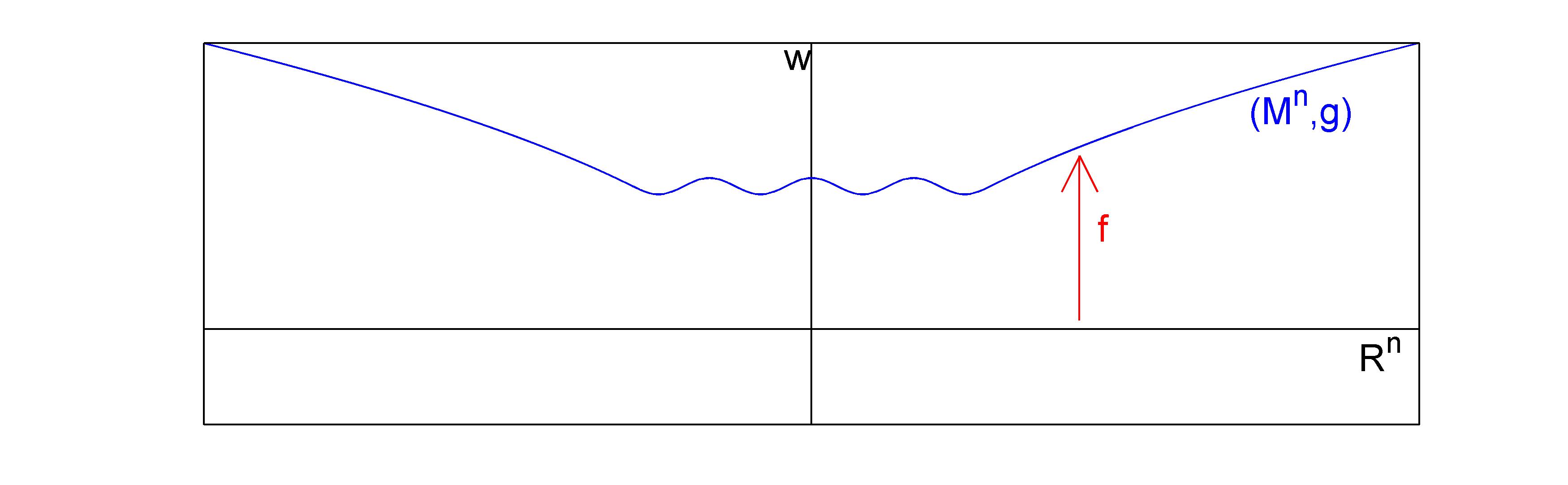
Figure 3: The graph of a real-valued function $f$ defined on ${\mathbb{R}}^{n}$ has a natural metric, namely the one induced from the flat background metric on ${\mathbb{R}}^{n+1}$. Lam’s work provides an explicit formula for the total mass of these Riemannian manifolds as an integral involving scalar curvature and $df$.

Given a smooth function $f:\mathbb{R}^{n}\to\mathbb{R}$, the graph of $f$ with metric induced from the flat metric on ${\mathbb{R}}^{n+1}$ is a complete Riemannian manifold isometric to $(\mathbb{R}^{n},\delta_{ij}+f_{i}f_{j})$, as sketched in figure 3. The following definition for an asymptotically flat function $f$ implies that the resulting graph manifold is asymptotically flat.

Definition 5.

[21, 22] Let $f:\mathbb{R}^{n}\to\mathbb{R}$ be a smooth function and let $f_{i}$ denote the $i$th partial derivative of $f$. We say that $f$ is asymptotically flat if

$$f_{i}(x) =O(|x|^{-p/2})$$

$$|x||f_{ij}(x)|+|x|^{2}|f_{ijk}(x)| =O(|x|^{-p/2})$$

at infinity for some $p>(n-2)/2$.

Lam is then able to derive an explicit expression for the total mass in terms of the scalar curvature of the graph, similar to equation 17 derived in the conformally flat manifold example.

Theorem 1 (Riemannian Positive mass inequality for Graphs over $\mathbb{R}^{n}$).

[21, 22] Let $(M^{n},g)$ be the graph of a smooth asymptotically flat function $f:\mathbb{R}^{n}\to\mathbb{R}$ with the induced metric from $\mathbb{R}^{n+1}$. Let $R$ be the scalar curvature and $m$ the total mass of $(M^{n},g)$. Let $dV_{g}$ denote the volume form on $(M^{n},g)$. Then

$$m=\int_{M^{n}}\frac{R}{2(n-1)\omega_{n-1}}\cdot\frac{1}{\sqrt{1+|\nabla f|^{2}}}\;dV_{g}.$$ (22)

In particular, $R\geq 0$ implies $m\geq 0$.

As in the conformally flat manifold example, the total mass is approximately the integral of scalar curvature divided by $2(n-1)\omega_{n-1}$ for perturbations of the flat metric corresponding to $df=0$. More generally, the total mass is less than this integral, roughly corresponding to the fact that potential energy is negative in Newtonian mechanics, as we also saw in the conformally flat example.

However, unlike the conformal examples, these graph examples can be extended to manifolds with boundaries to prove the Riemannian Penrose inequality in many graph cases as well, sketched in figure 4. To achieve this, the first step is the following theorem, which we note still gives an explicit expression for the total mass in terms of the scalar curvature and a boundary term.

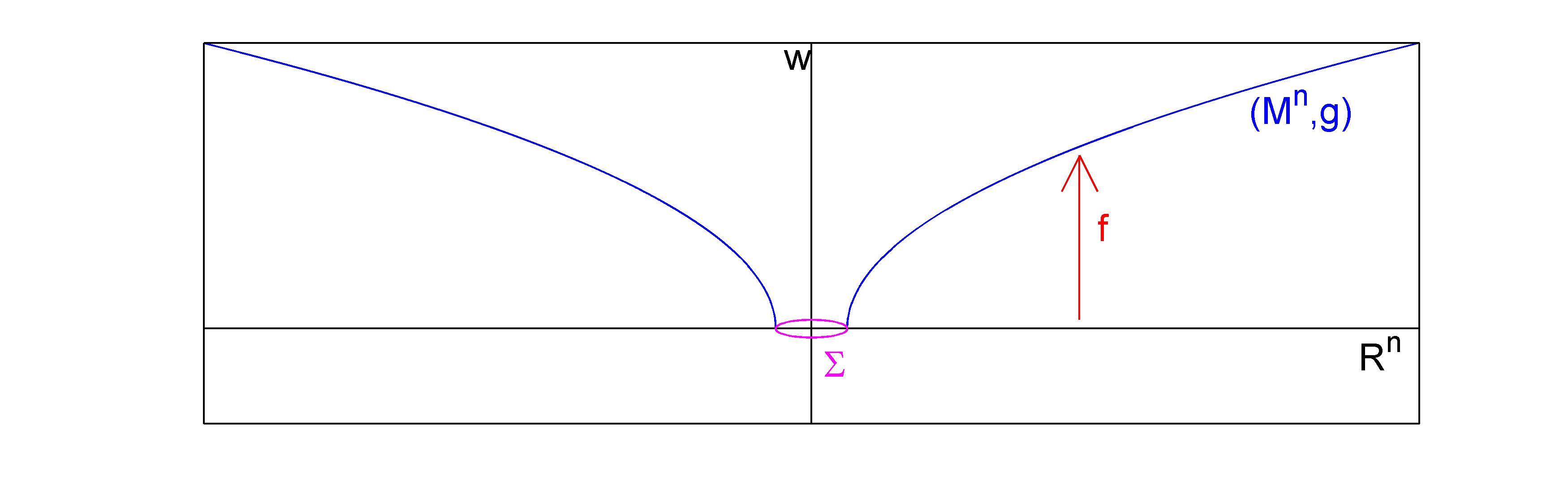
Figure 4: Same example as in the previous figure, but now the graph is allowed to have a vertical boundary. Lam’s previous result generalizes by gaining a boundary term, leading to a proof of the Riemannian Penrose inequality for these graph cases.

Theorem 2.

[21, 22] Let $\Omega$ be a bounded and open (but not necessarily connected) set with smooth boundary $\Sigma$ in $\mathbb{R}^{n}$. Let $f:\mathbb{R}^{n}\backslash\Omega\to\mathbb{R}$ be a smooth asymptotically flat function such that $\Sigma\subset f^{-1}(0)$ and $|\nabla f(x)|\to\infty$ as $x\to\Sigma$. Let $(M^{n},g)$ be the graph of $f$ with the induced metric from $(\mathbb{R}^{n}\backslash\Omega)\times\mathbb{R}$. Let $H$ be the mean curvature of $\Sigma$ in $(\mathbb{R}^{n},\delta)$ and $d\Sigma$ be the area form on $\Sigma$. Then the total mass of $(M^{n},g)$ is

$$m=\int_{\Sigma}\frac{Hd\Sigma}{2(n-1)\omega_{n-1}}+\int_{M^{n}}\frac{R}{2(n-1)\omega_{n-1}}\cdot\frac{1}{\sqrt{1+|\nabla f|^{2}}}\;dV_{g}.$$ (23)

The next step is to use a special case of the Aleksandrov-Fenchel inequality.

Lemma 1.

[33] If $\Sigma$ is a convex surface in $\mathbb{R}^{n}$ with mean curvature $H$ and area $|\Sigma|$, then

$$\frac{1}{2(n-1)\omega_{n-1}}\int_{\Sigma}Hd\Sigma\geq\frac{1}{2}\left(\frac{|\Sigma|}{\omega_{n-1}}\right)^{\frac{n-2}{n-1}}.$$ (24)

Putting the above two results together, Lam proves the Riemannian Penrose inequality in this case.

Corollary 1 (Riemannian Penrose Inequality for Graphs on $\mathbb{R}^{n}$ with Convex Boundaries).

[21, 22] With the same hypotheses as in Theorem 2, and the additional assumption that each connected component $\Omega_{i}$ of $\Omega$ is convex, then

$$m\geq\sum_{i=1}^{k}\frac{1}{2}\left(\frac{|\Sigma_{i}|}{\omega_{n-1}}\right)^{\frac{n-2}{n-1}}+\int_{M^{n}}\frac{R}{2(n-1)\omega_{n-1}}\cdot\frac{1}{\sqrt{1+|\nabla f|^{2}}}\;dV_{g},$$ (25)

where $\Sigma_{i}=\partial\Omega_{i}$. In particular, $R\geq 0$ implies that

$$m\geq\sum_{i=1}^{k}\frac{1}{2}\left(\frac{|\Sigma_{i}|}{\omega_{n-1}}\right)^{\frac{n-2}{n-1}}.$$ (26)

Equation 26 is actually stronger than the Riemannian Penrose inequality in general dimension, which is

$$m\geq\frac{1}{2}\left(\frac{\sum_{i=1}^{k}|\Sigma_{i}|}{\omega_{n-1}}\right)^{\frac{n-2}{n-1}}.$$ (27)

The inequality in equation 26 is not true in general and has explicit counterexamples. It is quite interesting that the “graph over ${\mathbb{R}}^{n}$” case is sufficiently restrictive to give this stronger result.

In fact, as far as the author is aware, the above theorem is all of the cases where the Riemannian Penrose inequality is known to be true when $n\geq 8$ since the graph cases include the spherically symmetric examples, which were the only cases known to the author prior to the above result. The general case of the Riemannian Penrose inequality is known in dimension $n\leq 7$ [4, 10], as discussed in the next section.

The key identity which Lam derived to prove the above results is a clever expression for the scalar curvature of graphs as the divergence of a vector field in the ${\mathbb{R}}^{n}$ base space. Direct computation shows that

$$R=\frac{1}{1+|\nabla f|^{2}}\left[f_{ii}f_{jj}-f_{ij}f_{ij}-\frac{2f_{j}f_{k}}{1+|\nabla f|^{2}}(f_{ii}f_{jk}-f_{ij}f_{ik})\right],$$ (28)

where subscripts denote partial differentiation in ${\mathbb{R}}^{n}$ and $\nabla$ is the gradient in ${\mathbb{R}}^{n}$. Denoting divergence in ${\mathbb{R}}^{n}$ as $\nabla\cdot$, Lam then proves the following result.

Lemma 2.

[21, 22] The scalar curvature of the graph $(\mathbb{R}^{n},\delta_{ij}+f_{i}f_{j})$ is

$$R=\nabla\cdot\left(\frac{1}{1+|\nabla f|^{2}}(f_{ii}f_{j}-f_{ij}f_{i})\partial_{j}\right).$$ (29)

Proof.

$$\nabla\cdot\left(\frac{1}{1+|\nabla f|^{2}}(f_{ii}f_{j}-f_{ij}f_{i})\partial_{j}\right)$$

$$= \frac{1}{1+|\nabla f|^{2}}(f_{iij}f_{j}+f_{ii}f_{jj}-f_{ijj}f_{i}-f_{ij}f_{ij})-\frac{2f_{jk}f_{k}}{(1+|\nabla f|^{2})^{2}}(f_{ii}f_{j}-f_{ij}f_{i})$$

$$= \frac{1}{1+|\nabla f|^{2}}\left[f_{ii}f_{jj}-f_{ij}f_{ij}-\frac{2f_{j}f_{k}}{1+|\nabla f|^{2}}(f_{ii}f_{jk}-f_{ij}f_{ik})\right]$$

$$= R$$

by (28). ∎

The key point is that the scalar curvature may be expressed as a divergence of a vector field, which is far from obvious from equation 28. This allows a divergence theorem argument to prove the desired results. We refer the reader to [21, 22] for the case where there is an interior boundary which leads to the Riemannian Penrose inequality. That case is a natural generalization of the case where there is no interior boundary. The no interior boundary case is used by Lam to prove the Riemannian positive mass inequality for manifolds which are graphs over ${\mathbb{R}}^{n}$, shown below.

Proof of Theorem 1.

By definition, the total mass of $(M^{n},g)=(\mathbb{R}^{n},\delta_{ij}+f_{i}f_{j})$ is

$$m =\lim_{r\to\infty}\frac{1}{2(n-1)\omega_{n-1}}\int_{S_{r}}(g_{ij,i}-g_{ii,j})\nu_{j}\;dS_{r}$$

$$=\lim_{r\to\infty}\frac{1}{2(n-1)\omega_{n-1}}\int_{S_{r}}(f_{ii}f_{j}+f_{ij}f_{i}-2f_{ij}f_{i})\nu_{j}\;dS_{r}$$

$$=\lim_{r\to\infty}\frac{1}{2(n-1)\omega_{n-1}}\int_{S_{r}}(f_{ii}f_{j}-f_{ij}f_{i})\nu_{j}\;dS_{r}.$$

By the asymtotic flatness assumption, the function $1/(1+|\nabla f|^{2})$ goes to 1 at infinity. Hence we can alternately write the mass as

$$m=\lim_{r\to\infty}\frac{1}{2(n-1)\omega_{n-1}}\int_{S_{r}}\frac{1}{1+|\nabla f|^{2}}(f_{ii}f_{j}-f_{ij}f_{i})\nu_{j}\;dS_{r}.$$

Now apply the divergence theorem in $(\mathbb{R}^{n},\delta)$ and use Lemma 1 to get

$$m =\frac{1}{2(n-1)\omega_{n-1}}\int_{\mathbb{R}^{n}}\nabla\cdot\left(\frac{1}{1+|\nabla f|^{2}}(f_{ii}f_{j}-f_{ij}f_{i})\partial_{j}\right)\;dV_{\delta}$$

$$=\frac{1}{2(n-1)\omega_{n-1}}\int_{\mathbb{R}^{n}}R\;dV_{\delta}$$

$$=\frac{1}{2(n-1)\omega_{n-1}}\int_{M^{n}}R\frac{1}{\sqrt{1+|\nabla f|^{2}}}\;dV_{g}$$

since

$$dV_{g}=\sqrt{\det(g)}\;dV_{\delta}=\sqrt{1+|\nabla f|^{2}}\;dV_{\delta}.$$

∎

We end this introduction by noting that Lam has generalized the identity in lemma 2 beyond ${\mathbb{R}}^{n}$, as is natural to do, as described in [21, 22]. It is of great interest to see what other applications this identity may have.

3 A Trio of Inequalities

In this section we describe the Riemannian positive mass inequality, the Riemannian Penrose inequality, and the Riemannian ZAS inequality. These three inequalities are intimately connected. Most obviously, the Schwarzschild metrics (of which there are precisely three up to scaling) are the cases of equality for these three inequalities.

In dimension two, the only reasonable interpretation of these three inequalities follows from the Gauss-Bonnet theorem (a natural story which we will not tell here). This is not surprising since the Gauss-Bonnet theorem is a global result about scalar curvature (equal to twice the Gauss curvature of a surface) as well. Hence, these theorems are, in a very real sense, nontrivial generalizations of the Gauss-Bonnet theorem to higher dimensions. Since the two dimensional case is somewhat exceptional and completely understood, we will always assume that $n\geq 3$.

All three inequalities are known to be true in dimension $n\leq 7$ [38, 10, 7] (assuming an interesting open conjecture for the Riemannian ZAS inequality [7], discussed later). Also, the only known proof of the Riemannian ZAS inequality in dimension $n\leq 7$ (modulo that interesting open conjecture [7]) requires the Riemannian Penrose inequality in dimension $n\leq 7$ [10], which in turn so far has only been proved using the Riemannian positive mass inequality in dimension $n\leq 7$ [38]. Hence, there appears to be a deep connection between these three inequalities.

3.1 The Riemannian Positive Mass Inequality

The Riemannian positive mass inequality is an elegant statement which reveals the global effect of nonnegative scalar curvature on an asymptotically flat manifold. Since scalar curvature is proportional to energy density in this context, the inequality equivalently states that nonnegative energy density implies nonnegative total mass. It also states that there is a unique zero total mass metric with nonnegative energy density, namely the flat metric on ${\mathbb{R}}^{n}$.

The Riemannian Positive Mass Inequality.

Let $(M^{n},g)$, $n\geq 3$, be a complete, asymptotically flat, smooth $n$-manifold with nonnegative scalar curvature and total mass $m$. Then

$$m\geq 0$$

with equality if and only if $(M^{n},g)$ is isometric to $\mathbb{R}^{n}$ with the standard flat metric.

Schoen and Yau surprised the relativity world in 1979 when they proved the Riemannian positive mass inequality in dimension three [37] because the techniques they used were based on existence and stability properties of minimal surfaces. A nice discussion of these techniques, as well as related results including a fascinating discussion of the hyperbolic version of the positive mass theorem, is provided in [15], also in this book dedicated to Rick Schoen’s 60th birthday. In [38], Schoen and Yau extended their argument using Jang’s equation to prove the more general positive mass inequality for a generic slice of a spacetime, in dimension three. In addition, Schoen and Yau showed that their argument extended to dimensions less than eight by using a minimal hypersurface argument which is inductive on dimension [36, 35]. The higher dimension Jang equation argument which proves the higher dimensional positive mass inequality in dimensions less than eight is treated very carefully in [13], following the method suggested by [38]. However, another initially surprising fact is that minimal hypersurfaces may have singularities on a subset whose codimension has been proven to be at least seven [39, 14, 40, 3], which prevented [36, 35] from proving the Riemannian positive mass inequality for manifolds in dimension eight and higher. However, in 2009 Schoen has been giving talks [34] about an approach to overcoming this obstacle by trying to show that the minimal hypersurface singularities can be sufficiently controlled. If this approach is ultimately successful, this would prove the Riemannian positive mass inequality in all dimensions.

In addition, Lohkamp has studied a somewhat different way of modifying the original Schoen-Yau minimal surface argument. He announced a proof of the positive mass inequality in all dimensions around or before 2004 which he describes in a 2006 preprint [24]. The techniques involved have been further expanded upon in followup preprints [11, 25].

Meanwhile, Witten’s 1981 proof [41, 29] of the positive mass inequality works in all dimensions, but only for manifolds which are spin. So far no one has been able to get around this extra topological assumption using a spinor approach.

Also, Lam’s results [21, 22], described at the end of the previous section, work in general dimension and imply both the Riemannian positive mass inequality and the Riemannian Penrose inequality for certain manifolds which can be realized as graphs over ${\mathbb{R}}^{n}$. Naturally this assumption is very restrictive, but the results are very good for helping to develop intuition.

Finally, in dimension three, the inverse mean curvature flow techniques of Huisken and Ilmanen [18] prove the Riemannian positive mass inequality by starting the inverse mean curvature flow on a surface which is a small geodesic sphere around a fixed point, in the limit as the radius of the geodesic sphere goes to zero. In fact, Lemma 8.1 of [18] proves that there is a solution to inverse mean curvature flow starting at a point, from which the Riemannian positive mass inequality in dimension three follows. Huisken and Ilmanen show that their inverse mean curvature flow exists in dimensions less than eight. However, the monotonicity of the Hawking mass of the surfaces in the flow, a critical component of their proof of the Riemannian positive mass inequality in dimension three, is only always satisfied in dimension three. It is a fascinating open question whether or not this type of approach could work in dimensions greater than three.

In [23], Lohkamp makes a nice connection between asymptotically flat manifolds and compact manifolds in the context of scalar curvature by proving the following:

Lemma 3.

[23] Let $(M^{n},g)$ be a complete, asymptotically flat, smooth manifold, and let $\tilde{M}^{n}$ be the compact smooth manifold which results from compactifying $M^{n}$ by adding a point at infinity. If $T^{n}\#\tilde{M}^{n}$ does not admit a metric of positive scalar curvature, then the Riemannian positive mass inequality is true for $(M^{n},g)$.

To be clear, we mean to say that if $(M^{n},g)$ has nonnegative scalar curvature, then its total mass is nonnegative. The case of equality when the total mass is zero is also true by a short time Ricci flow / conformal change argument [37, 2] which we do not present here.

Hence, the Riemannian positive mass inequality may be approached by studying topological obstructions to compact manifolds admitting metrics of positive scalar curvature. We refer the reader to [15] for more discussion. Besides this topological question being interesting in its own right, the Riemannian positive mass theorem in all dimensions would follow from proving that $T^{n}\#M^{n}$ does not admit a metric of positive scalar curvature for any compact $M^{n}$.

Lohkamp’s lemma may be proved as follows. Let $(M^{n},g)$ be complete, smooth, and asymptotically flat with nonnegative scalar curvature. Suppose that the total mass $m<0$. Then Lohkamp shows that the metric $g$ may be perturbed to a new metric $\tilde{g}$ while preserving nonnegative scalar curvature such that outside a bounded set $\tilde{g}$ is flat. Choosing a cube which contains this bounded set and identifying the opposite sides produces a metric $\tilde{\tilde{g}}$ on $T^{n}\#\tilde{M}^{n}$ with nonnegative scalar curvature. Furthermore, the perturbation process produces a region where the scalar curvature of $\tilde{\tilde{g}}$ is strictly positive. Multiplying $\tilde{\tilde{g}}$ through by the correct conformal factor close to one spreads out this positive scalar curvature so that the new conformal metric has positive scalar curvature everywhere. But $T^{n}\#\tilde{M}^{n}$ does not admit a metric of positive scalar curvature, so we have a contradiction. Hence, we can not have $m<0$, so $m\geq 0$.

For the case of equality, suppose $m=0$. Then the previously mentioned short time Ricci flow / conformal change argument [37] decreases the total mass to being negative unless the manifold is Ricci flat. The fact that Ricci flat plus asymptotically flat implies flat is in [2]. Since the total mass can not be negative by the above paragraph, it must be that $(M^{n},g)$ is isometric to the flat metric on ${\mathbb{R}}^{n}$.

The key step in the above proof is to take the asymptotically flat metric $g$ with negative total mass and to perturb it while preserving nonnegative scalar curvature to get the metric $\tilde{g}$ which is flat outside a bounded set. Besides Lohkamp’s construction [23], one can also use one of the author’s thesis results [6] (based on the harmonically flat perturbation result [38] of Schoen and Yau) that allows an asymptotically flat manifold to be perturbed to being Schwarzschild at infinity while preserving nonnegative scalar curvature and changing the total mass as little as one likes, so that in this case the total mass stays negative. Since Schwarzschild is spherically symmetric, the metric can then be “curved up” to being precisely flat outside a bounded set in the space of spherically symmetric metrics with nonnegative scalar curvature, which is most easily seen by considering the Hawking masses of the spherically symmetric spheres.

3.2 The Riemannian Penrose Inequality

The Riemannian Penrose inequality is another elegant statement which, like the Riemannian positive mass inequality, reveals the global effect of nonnegative scalar curvature on an asymptotically flat manifold, but where now there may be an interior boundary. Conditions imposed on this interior boundary allow each connected component of the boundary to be interpreted physically as the apparent horizon of a black hole. As before, scalar curvature is proportional to energy density at each point. Now suppose that we define the mass contributed by this collection of black holes in terms of the $(n-1)$ volume of the boundary. In doing so, we may interpret the Riemannian Penrose inequality as the physical statement that nonnegative energy density implies that the total mass is at least the mass contributed by the black holes.

The Riemannian Penrose Inequality.

Let $(M^{n},g)$, $n\geq 3$, be a complete, asymptotically flat, smooth $n$-manifold with nonnegative scalar curvature, total mass $m$, and a strictly outerminimizing smooth minimal boundary which is compact (but not necessarily connected) of total $(n-1)$ volume $A$. Then

$$m\geq\frac{1}{2}\left(\frac{A}{\omega_{n-1}}\right)^{\frac{n-2}{n-1}}$$ (30)

with equality if and only if $(M^{n},g)$ is isometric to the region of a Schwarzschild metric of positive mass outside its minimal hypersurface.

In the above statement, $\omega_{n-1}$ is the measure of the unit $(n-1)$ sphere in ${\mathbb{R}}^{n}$. A minimal boundary is one which has zero mean curvature. Finally, strictly outerminimizing means that all other smooth hypersurfaces in the same homology class have greater $(n-1)$ volume.

We hasten to add that it may be of considerable interest and importance to study versions of the above statement where the smoothness of the boundary is removed, and the notion of being minimal is revisited. For example, in dimensions eight and higher, minimizing hypersurfaces may have singularities on a subset whose codimension has been proven to be at least seven [39, 14, 40, 3], so a more general notion of allowable boundaries could be very important.

The Riemannian Penrose inequality was effectively conjectured by Penrose [30] in 1973. The inequality was proved in dimension less than eight [10] in 2007 by Lee and the author (both former students of Rick Schoen, it should be noted in this birthday volume) by generalizing the conformal flow of metrics method originally used in the author’s 1999 proof of the inequality in dimension three [4]. The difficulty in pushing the argument through to dimensions greater than seven is, once again, that minimal hypersurfaces may have singularities on a subset whose codimension has been proven to be at least seven [39, 14, 40, 3]. Proving the Riemannian Penrose inequality in dimensions greater than seven is an excellent open problem.

We refer the reader to [5] for a general discussion of the conformal flow of metrics technique. The basic idea is to flow the starting manifold $(M^{n},g)$ to a Schwarzschild metric while preserving nonnegative scalar curvature in such a way that the $(n-1)$ volume of the boundary remains fixed and the total mass is nonincreasing. The Riemannian Penrose inequality is defined to give equality for the Schwarzschild metrics, so the inequality for the original starting manifold follows. The surprising fact is that it is possible to do this flow inside the conformal class of the original manifold, which could even have a different topology than the Schwarzschild metric. The solution is to allow the boundary to be a moving boundary, where in the limit as the flow time goes to infinity, the moving boundary (which sometimes jumps over regions and topology) goes to infinity as well, eventually enclosing any bounded set. Another important characteristic of the conformal flow of metrics approach is that the monotonicity of the total mass is, quite beautifully, a direct and yet nontrivial consequence of the Riemannian positive mass theorem, as described in [4, 5].

An earlier breakthrough on the Riemannian Penrose inequality was due to Huisken and Ilmanen [18] in 1997 using a technique called inverse mean curvature flow, which proved the inequality in dimension three when the minimal boundary is connected and outermost (not enclosed by any other minimal surface). Inverse mean curvature flow is of great independent interest as well. In the seventies, Geroch [16] and Jang and Wald [19] proposed this novel approach to address the Riemannian Penrose inequality by flowing surfaces with speed equal to the reciprocal of their mean curvatures at each point. Amazingly, there is an explicit quantity called the Hawking mass which is nondecreasing under this flow, in dimension three, and which equals the right and left sides of the Riemannian Penrose inequality at $t=0$ and $t=\infty$, respectively. However, Geroch, Jang, and Wald did not prove a general existence theory for this flow, which is understandable because there are examples of manifolds and initial surfaces where it is known that smooth solutions to inverse mean curvature flow do not exist. Hence, it was quite surprising and a true breakthrough in 1997 when Huisken and Ilmanen found a weak notion of inverse mean curvature flow which allowed the surfaces to occasionally jump while still preserving the monotonicity of the Hawking mass [18].

The monotonicity of the Hawking mass turns out to rely on the two dimensional Gauss-Bonnet formula for the surfaces in the flow which need to have Euler characteristic not exceeding two. Consequently, the argument so far only works in dimension three. It is a fascinating open question whether or not this type of approach could work in dimensions greater than three. However, by a result due to Meeks, Simon, and Yau [27], the exterior region outside the outermost minimal surface of an asymptotically flat 3-manifold is, quite remarkably, always diffeomorphic to ${\mathbb{R}}^{3}$ minus a finite number of disjoint closed balls. Huisken and Ilmanen start their inverse mean curvature flow on the boundary of one of these balls so that the initial Euler characteristic equals two, and then use the trivial topology of the exterior region to guarantee that the surfaces resulting from their weak inverse mean curvature flow stay connected, and hence continue to have Euler characteristic not exceeding two. The Riemannian Penrose inequality follows, where $A$ is the area of any of the connected components of the outermost minimal surface of the manifold. We refer the reader to [18, 5] for more discussion of inverse mean curvature flow.

In dimension greater than eight, Lam’s proof of the Riemannian Penrose inequality for manifolds which are graphs over ${\mathbb{R}}^{n}$ is all of the cases where the Riemannian Penrose inequality is known to be true, as far as the author is aware. Previously the inequality was only known in the spherically symmetric case in these higher dimensions, which may also be realized as graphs in Lam’s examples.

To push the physical interpretation of the Riemannian Penrose inequality a little further, let $\Sigma_{BH}$ be the minimal boundary with connected components $\{\Sigma_{BH}^{i}\}$, each of which we will think of as the apparent horizon of a black hole (which is the case when $\Sigma$ is the outermost minimal hypersurface). Then if we define the mass contributed by this collection of black holes to be

$$m_{BH}=\frac{1}{2}\left(\frac{|\Sigma_{BH}|}{\omega_{n-1}}\right)^{\frac{n-2}{n-1}},$$ (31)

where $|\Sigma_{BH}|$ is the $(n-1)$ volume of the boundary $\Sigma_{BH}$, then the Riemannian Penrose inequality may be stated as

$$m\geq m_{BH},$$ (32)

that the total mass is at least the mass contributed by the black holes.

We also refer the reader to [26] for Marc Mars’s excellent survey of results on the Penrose inequality, a more general statement about spacelike hypersurfaces $M^{n}$ of spacetimes $(N^{n+1},g_{N})$ involving the second fundamental form $k$ and the induced metric $g$ on $M^{n}$. We note that when the second fundamental form $k$ is zero, the relevant data is $(M^{n},g)$, a Riemannian manifold. This observation inspired Huisken and Ilmanen [18] to refer to the zero second fundamental form case of the Penrose inequality as the Riemannian Penrose inequality, by which it has been known ever since. The full Penrose inequality, or Penrose conjecture, is a very important open problem since it says something very interesting about the geometries of spacetimes. In [8, 9], Khuri and the author propose an approach to reduce the full Penrose inequality (which is still wide open) to the Riemannian Penrose inequality (which has been proven in dimensions less than eight). The key step is the derivation of a new identity, called the generalized Schoen-Yau identity, which is a nontrivial generalization of an identity first proved by Schoen and Yau in their proof of the positive mass inequality [38]. We stop here because, while it would have been very tempting to survey recent progress on the Penrose inequality for this volume, Marc Mars’s recent survey [26] makes this completely unnecessary.

3.3 The Riemannian ZAS Inequality

The Riemannian ZAS inequality is the last of our trio of inequalities. Like the Riemannian Penrose inequality and the Riemannian positive mass inequality, the Riemannian ZAS inequality describes the global effect of nonnegative scalar curvature on an asymptotically flat manifold. The new feature, however, is that our manifold is now allowed to have a finite number of isolated singularities. In [7], Jauregui and the author define a notion of the mass contributed by a finite collection of zero area singularities (ZAS), which is very general. The total mass of an asymptotically flat manifold with nonnegative scalar curvature is then shown to be at least the mass contributed by the singularities, whenever a certain geometric conjecture is true. We refer the interested reader to [7] for the details but survey some of the main points from that paper here. We comment that [7] focused on $n=3$, whereas we are presenting the general dimension case here (with Jauregui’s help), which is a natural generalization. We also comment that of the three inequalities, the Riemannian ZAS inequality is the least well understood with many excellent problems left open and plenty of interesting directions to explore.

Another interesting point is that the Riemannian ZAS inequality is primarily motivated by geometric considerations as opposed to physical ones. While well established physical reasoning led to the conjecturing of the positive mass inequality and the Penrose inequality, the Riemannian ZAS inequality, as we pose it here, has simply been defined to be what can be proved mathematically so far. In fact, a precise statement of what the ZAS inequality should be exactly has not yet been established beyond the Riemannian case (although there are some natural candidates), and even the Riemannian case is not perfectly clear. Hence, it is not yet evident what the physical implications of this inequality, if any, will be, although the discussion of singularities in general relativity is well underway [17, 12].

As promised, the Schwarzschild metrics with negative mass are cases of equality of the Riemannian ZAS inequality. Metrically, these singularities look like a cusp at a single point, as in figure 2. Note that the singularity is not roughly conical in the usual sense as the picture suggests since the background metric is Minkowski space and the hypersurface is becoming null at the singularity. Also, referring back to equation 8, one sees that the singularity of a negative mass Schwarzschild metric occurs on the coordinate sphere of radius $r=(|m|/2)^{\frac{1}{n-2}}>0$ since the conformal factor goes to zero on this sphere. In fact, it is useful to think of these singularities as surfaces with zero area.

Definition 6.

[7] Let $M^{n}$ be a smooth $n$-manifold with smooth compact boundary $\partial M$ and let $g$ be a complete, smooth, asymptotically flat metric on $M\backslash\partial M$. A connected component $\Sigma$ of $\partial M$ is a zero area singularity (ZAS) of $(M^{n},g)$ if for every sequence of surfaces $\{S_{n}\}$ converging in $C^{1}$ to $\Sigma$, the areas of $S_{n}$ measured with respect to $g$ converge to zero.

In this section we will consider the case when every connected component of $\partial M$ is a ZAS, so we define $\Sigma_{ZAS}=\partial M$. As one might expect, not all singularities have equally bad behavior, even when curvatures are blowing up to infinity. In [7], notions of regular ZAS, harmonically regular ZAS, and globally harmonically regular ZAS are defined.

Definition 7.

[7] Let $\Sigma$ be a ZAS of $(M^{n},g)$. Then $\Sigma$ is regular if there exists a smooth, nonnegative function $\overline{\varphi}$ and a smooth metric $\overline{g}$, both defined on a neighborhood $U$ of $\Sigma$ (which of course includes $\Sigma$), such that

(1) $\overline{\varphi}$ vanishes precisely on $\Sigma$,

(2) $\overline{\nu}(\overline{\varphi})>0$ on $\Sigma$, where $\overline{\nu}$ is the inward unit normal to $\Sigma$ with respect to $\overline{g}$,

(3) $g=\overline{\varphi}^{\,4/(n-2)}\overline{g}$ on $U\backslash\Sigma$.

If such a pair $(\overline{g},\overline{\varphi})$ exists, it is called a local resolution of $\Sigma$.

When $\overline{\varphi}$ is also harmonic with respect to $\overline{g}$, then the ZAS is defined to be harmonically regular with a local harmonic resolution. Finally, if all of the connected components of $\partial M$ are harmonically regular ZAS with the same $\overline{\varphi}$, where $U$ is the entire manifold, then all of the ZAS are defined to be globally harmonically regular with a global harmonic resolution. Note that the negative mass Schwarzschild metric singularity is globally harmonically regular (and hence harmonically regular and regular), as can be seen from equation 8. However, there are regular ZAS which are not harmonically regular (section 4.4 of [7]).

These notions of regular ZAS are useful because generic ZAS may be approximated by them, as described in [7]. In doing so, the definition of the mass of a regular ZAS may be extended to give a definition of the mass of a generic ZAS. We refer the reader to [7] for these and other discussions.

Definition 8.

Suppose $\Sigma$ is a regular ZAS of $(M^{n},g)$ with local resolution $(\overline{g},\overline{\varphi})$. We define the regular mass of $\Sigma$ to be

$$m_{reg}(\Sigma)=-\frac{2}{(n-2)^{2}}\left(\frac{1}{\omega_{n-1}}\int_{\Sigma}({\overline{\nu}}(\overline{\varphi}))^{\frac{2(n-1)}{n}}\;\overline{dA}\right)^{\frac{n}{n-1}},$$ (33)

where ${\overline{\nu}}$ is the inward unit normal to $\Sigma$ with respect to $\overline{g}$, $\overline{dA}$ is the $(n-1)$ volume form of $\overline{g}$, and $\omega_{n-1}$ is the $(n-1)$ volume of the unit $(n-1)$ sphere in ${\mathbb{R}}^{n}$.

Again, this definition of the mass of a regular ZAS was chosen primarily because theorems can be proved about it. Hence, other definitions should also be considered. However, in addition to being able to prove theorems using this definition, it also gives the correct answer in the case of a negative mass Schwarzschild singularity, namely $-|m|$, is independent of the particular choice of local resolution, and only depends on the local geometry near the singularity. The local nature of this definition of the mass of a regular ZAS is best seen by this next lemma (proposition 12 in [7]). In fact, one could take the following formula to be the definition of the mass of a regular ZAS, if one prefers.

Lemma 4.

Suppose $\Sigma$ is a regular ZAS of $(M^{n},g)$. If $\{\Sigma_{n}\}$ is a sequence of surfaces converging to $\Sigma$ in $C^{2}$, then

$$m_{reg}(\Sigma)=\lim_{n\rightarrow\infty}-\frac{1}{2(n-1)^{2}}\left(\frac{1}{\omega_{n-1}}\int_{\Sigma_{n}}H^{\frac{2(n-1)}{n}}\;dA\right)^{\frac{n}{n-1}},$$ (34)

where $H$ is the mean curvature of $\Sigma_{n}$, and $dA$ is the $(n-1)$ volume form on $\Sigma_{n}$.

We define the mass contributed by a collection of regular ZAS using equations 33 and 34, where $\Sigma=\Sigma_{ZAS}=\partial M$ may now have multiple components. That is, we define

$$m_{ZAS}=m_{reg}(\Sigma_{ZAS}).$$ (35)

Again, we refer the reader to [7] for the case of generic ZAS. In all cases, the goal is to prove that $m\geq m_{ZAS}$, that is, that the total mass of a complete, asymptotically flat, smooth $n$-manifold with smooth boundary, each connected component of which is a ZAS, is at least the mass contributed by the ZAS.

The Riemannian ZAS Inequality.

Let $(M^{n},g)$, $n\geq 3$, be a complete, asymptotically flat, smooth $n$-manifold with nonnegative scalar curvature, total mass $m$, and nonempty compact boundary $\partial M$ (smooth with respect to the smooth structure), each connected component of which is a ZAS. Then

$$m\geq m_{ZAS}$$ (36)

with equality if and only if $(M^{n},g)$ is isometric to a Schwarzschild metric of negative mass.

The Riemannian ZAS inequality in dimension three is proven in [7] whenever a certain geometric conjecture, called the conformal conjecture, is true. The proof in [7] generalizes to dimensions less than eight without any significant changes. We state the conformal conjecture more generally than in [7] to emphasize what is needed to be true for the method in [7] to work.

The Conformal Conjecture.

Let $(M^{n},g)$, $n\geq 3$, be a complete, asymptotically flat, smooth $n$-manifold with nonempty compact boundary $\Sigma=\partial M$ which is smooth with respect to the smooth structure and the metric $g$. Then there exists a positive harmonic function $u(x)$ on $(M^{n},g)$ going to one at infinity such that if we let $\overline{g}=u(x)^{4/(n-2)}g$ and $\tilde{\Sigma}$ be the outermost minimal enclosure of $\Sigma$ in $(M^{n},\overline{g})$, then

(1) $\tilde{\Sigma}$ and $\Sigma$ have the same $(n-1)$ volume in $(M^{n},\overline{g})$,

(2) $\tilde{\Sigma}$ has zero mean curvature, at least in some weak sense compatible with the Riemannian Penrose inequality.

The power of the conformal conjecture, when it is true, is that it allows one to apply the Riemannian Penrose inequality to any asymptotically flat manifold with nonnegative scalar curvature and compact boundary to gain some information about the manifold. If the original metric has nonnegative scalar curvature, then since

$$\overline{R}=u(x)^{-\frac{n+2}{n-2}}\left(-\frac{4(n-1)}{n-2}\Delta u+Ru\right),$$ (37)

the new metric $\overline{g}$ will have nonnegative scalar curvature as well. It turns out to be too much to ask that the boundary $\Sigma$ satisfies the conditions of the Riemannian Penrose inequality (being a strictly outerminimizing minimal surface). Instead, the conjecture simply asks $\Sigma$ to have the same $(n-1)$ volume as its outermost minimal enclosure $\tilde{\Sigma}$, which is automatically strictly outerminimizing by definition. Hence, if the conjecture is satisfied, and $\tilde{\Sigma}$ has zero mean curvature, at least in some weak sense compatible with the Riemannian Penrose inequality, then we can effectively apply the Riemannian Penrose inequality to $\Sigma$, since it has the same $(n-1)$ volume as $\tilde{\Sigma}$. This inequality then gives information about the original manifold $(M^{n},g)$, for example proving the Riemannian ZAS inequality as described in [7] (when combined with some additional arguments), when the ZAS are globally harmonically regular. A process by which generic ZAS are approximated by globally harmonically regular ZAS then proves the Riemannian ZAS inequality in dimension less than eight, whenever the conformal conjecture is true.

We note that the conformal conjecture is true when $(M^{n},g)$ is spherically symmetric, which is a good exercise. Also, a substantial amount of progress has been made on the conformal conjecture in Jauregui’s thesis [20], which proves that a conformal factor may be chosen so that $\tilde{\Sigma}$ has zero mean curvature off a set of measure zero. As we commented before, it may be important to study versions of the Riemannian Penrose inequality where the smoothness of the boundary is not required. Finding the most general allowable boundary conditions for the Riemannian Penrose inequality could be a very interesting and important open problem, potentially with implications for the Riemannian ZAS inequality.

In the case of a single ZAS in dimension three, Huisken and Ilmanen’s inverse mean curvature flow proves the Riemannian ZAS inequality, as shown by Robbins in [31, 32]. However, if there is more than one ZAS, then no conclusion results from inverse mean curvature flow. The reason is that the Hawking mass is only nondecreasing if the surfaces in the flow are connected. Hence, the flow must start at one of the ZAS. However, when the surfaces flow over the other ZAS, the Hawking mass will not be nondecreasing. Once could hope that the inverse mean curvature flow might always jump over the other ZAS, but this is not the case, since we know that the total mass can in fact be less than the mass of any single ZAS. More realistically, one could hope to estimate how much the Hawking mass decreases when the surfaces flow over the other ZAS. This could be an interesting problem to study. It is even possible that the surfaces in the flow get “snagged” on ZAS for a positive amount of time in the flow when they pass over ZAS, which would be another interesting phenomenon to study.

Also, when $(M^{n},g)$ is isometric to a graph over ${\mathbb{R}}^{n}$ in $(n+1)$ dimensional Minkowski space, Lam’s methods [21, 22] prove a version of the ZAS inequality when ZAS are present, as in figure 2. This argument works for any number of ZAS in any dimension.

We comment that equations 31 and 35 combine to motivate defining the quasi-local mass functional

$${\mathcal{M}}(S)=\frac{1}{2}\left(\frac{|S|}{\omega_{n-1}}\right)^{\frac{n-2}{n-1}}\;-\;\;\frac{1}{2(n-1)^{2}}\left(\frac{1}{\omega_{n-1}}\int_{S}H^{\frac{2(n-1)}{n}}\;dA\right)^{\frac{n}{n-1}}$$ (38)

for a compact hypersurface $S$, where $|S|$ is the $(n-1)$ volume of $S$, $H$ is the mean curvature of $S$, and $dA$ is the $(n-1)$ volume form on $S$. The virtue of this quasi-local mass functional ${\mathcal{M}}$ is that on a collection of minimal hypersurfaces (where $H=0$) it gives the mass contributed by a collection of black holes as in equation 31 and in the limit as $S$ converges to a collection of ZAS in $C^{2}$ (where $|S|$ is going to zero) it gives the mass contributed by a collection of ZAS as in equation 35. Furthermore, ${\mathcal{M}}(S)=m$ for any of the spherically symmetric spheres $S$ of a Schwarzschild metric of mass $m$. However, the author is not aware of any flow which makes this functional nondecreasing. The big open problem is to try to generalize the successes of inverse mean curvature flow and the fact that it makes the Hawking mass functional nondecreasing to general dimension and to surfaces which are not necessarily connected.

Another interesting conjecture to study, again motivated by equations 31 and 35, is one which combines the Riemannian Penrose inequality with the Riemannian ZAS inequality, which we will state as

$$m\geq m_{BH}+m_{ZAS}.$$ (39)

In the above combined black hole ZAS conjecture, we are assuming that every connected component of the boundary of the smooth topological manifold $M^{n}$ is either a strictly outerminimizing minimal hypersurface (corresponding to the apparent horizon of a black hole) or a ZAS. Note that the masses of black holes do not “add” in that there are examples of asymptotically flat manifolds where

$$m<\frac{1}{2}\left(\frac{|\Sigma_{BH}^{1}|}{\omega_{n-1}}\right)^{\frac{n-2}{n-1}}+\frac{1}{2}\left(\frac{|\Sigma_{BH}^{2}|}{\omega_{n-1}}\right)^{\frac{n-2}{n-1}},$$ (40)

where the boundary of the manifold is a strictly outerminimizing minimal hypersurface with connected components $\Sigma_{BH}^{1}$ and $\Sigma_{BH}^{2}$. Similarly, the masses of ZAS do not “add” either. Essentially, the reason is related to the fact that the potential energy between two objects in Newtonian physics is $-Gm_{1}m_{2}/r^{n-2}$, which is negative when the two masses have the same sign. However, this potential energy term is positive when the two masses have opposite signs. Inspired by this, the above conjecture that the total mass is at least the sum of the mass contributed by the collection of black holes with the mass contributed by the collection of ZAS seems plausible, and hence deserving of further study. Note that another way to state this conjecture, using the quasi-local mass function just defined, is as $m\geq{\mathcal{M}}(\partial M)$. Conjecturally, the cases of equality would be the Schwarzschild metrics of any mass, positive or negative. In addition, the metric on ${\mathbb{R}}^{n}$ (minus some compact set) given by

$$g_{ij}=\left(1+\frac{m_{1}}{2|x-x_{1}|^{n-2}}+\frac{m_{2}}{2|x-x_{2}|^{n-2}}\right)^{\frac{4}{n-2}}\delta_{ij}$$ (41)

in the limit as $x_{1},x_{2}\in{\mathbb{R}}^{n}$ get infinitely far apart, are arbitrarily close to being cases of equality, when $m_{1}$ and $m_{2}$ have opposite signs, corresponding to precisely one black hole and one ZAS. This last observation could be an important hint for approaching this combined black hole ZAS conjecture.

The author would like to thank Michael Eichmair, Jeff Jauregui, George Lam, Dan Lee, and Fernando Schwartz for helpful suggestions with this paper, all of whom join the author in wishing Rick a very happy 60th birthday.

References

- [1] R. Arnowitt, S. Deser, C. W. Misner, “The Dynamics of General Relativity,” Gravitation: An Introduction to Current Research, pages 227-265. Wiley, New York, 1962.
- [2] R. Bartnik, “The Mass of an Asymptotically Flat Manifold,” Comm. Pure Appl. Math.,39(5):661-693, 1986.
- [3] E. Bombieri, E. De Giorgi, E. Giusti, “Minimal Cones and the Bernstein Problem,” Invent. Math. 7 (1969) 243-268.
- [4] H. L. Bray, “Proof of the Riemannian Penrose Inequality Using the Positive Mass Theorem,” J. Diff. Geom., 59(2):177-267, 2001.
- [5] H. L. Bray, “Black Holes, Geometric Flows, and the Penrose Inequality in General Relativity,” Notices of the American Mathematical Society, vol. 49 no. 11 (2002), pp. 1372–1381.
- [6] H. L. Bray, “The Penrose Inequality in General Relativity and Volume Comparison Theorems Involving Scalar Curvature,” 1997, thesis, Stanford University, [arXiv:0902.3241v1] (http://arxiv.org/abs/0902.3241).
- [7] H. L. Bray, J. L. Jauregui, “A Geometric Theory of Zero Area Singularities in General Relativity,” arXiv:0909.0522v1 [math.DG] (http://arxiv.org/abs/0909.0522).
- [8] H. L. Bray, M. A. Khuri, “P.D.E.’s which Imply the Penrose Conjecture,” arXiv:0905.2622v1 [math.DG] (http://arxiv.org/abs/0905.2622).
- [9] H. L. Bray, M. A. Khuri, “A Jang Equation Approach to the Penrose Inequality,” Discrete Contin. Dyn. Syst. 27 (2010), no. 2, 741–766, arXiv:0910.4785v1 [math.DG] (http://arxiv.org/abs/0910.4785).
- [10] H. L. Bray, D. A. Lee, “On the Riemannian Penrose Inequality in Dimensions Less Than Eight,” Duke Mathematical Journal, vol. 148, no. 1 (2009), pp. 81-106, arXiv:0705.1128v1 [math.DG] (http://arxiv.org/abs/0705.1128).
- [11] U. Christ, J. Lohkamp, “Singular Minimal Hypersurfaces and Scalar Curvature,” arXiv:math/0609338v1 [math.DG], 2006.
- [12] G. Dotti, R. J. Gleiser, “The Initial Value Problem for Linearized Gravitational Perturbations of the Schwarzschild Naked Singularity,” arXiv:0809.3615v3 [gr-qc] (http://arxiv.org/abs/0809.3615).
- [13] M. Eichmair, “The Space-Time Positive Mass Theorem in Dimensions Less Than Eight” (in preparation).
- [14] H. Federer, Geometric Measure Theory, Die Grundlehren der mathematischen Wissenschaften, Band 153, Springer-Verlag New York Inc., New York, 1969.
- [15] G. Galloway, “Stability and Rigidity of Extremal Surfaces in Riemannian Geometry and General Relativity,” Surveys in Geometric Analysis and Relativity Celebrating Richard Schoen’s 60th birthday, Higher Education Press and International Press Beijing-Boston, 2010.
- [16] R. Geroch, “Energy Extraction,” D. J. Hegyi, editor, Sixth Texas Symposium on Relativistic Astrophysics, volume 224 of New York Academy Sciences Annals, 1973.
- [17] G. W. Gibbons, S. A. Hartnoll, A. Ishibashi, “On the Stability of Naked Singularties,” Prog. Theor. Phys. 113:963-978, 2005, arXiv:hep-th/0409307v1 (http://arxiv.org/abs/hep-th/0409307).
- [18] G. Huisken, T. Ilmanen, “The Inverse Mean Curvature Flow and the Riemannian Penrose Inequality,” J. Diff. Geom., 59(3):353-437, 2001.
- [19] P. S. Jang, R. M. Wald, “The Positive Energy Conjecture and the Cosmic Censor Hypothesis,” Journal of Mathematical Physics, 18:41-44, Jan. 1977.
- [20] J. L. Jauregui, “Mass Estimates, Conformal Techniques, and Singularities in General Relativity,” thesis, Duke University, 2010.
- [21] G. Lam, thesis, in preparation, Duke University, 2011 (expected).
- [22] G. Lam, “Proof of the Graph Cases of the Riemannian Positive Mass Theorem and the Riemannian Penrose Inequality in All Dimensions,” (in preparation).
- [23] J. Lohkamp, “Scalar Curvature and Hammocks,” Math. Ann., 313(3):385-407, 1999.
- [24] J. Lohkamp, “The Higher Dimensional Positive Mass Theorem I,” arXiv.org:math/0608795, 2006.
- [25] J. Lohkamp, “Inductive Analysis on Singular Minimal Hypersurfaces,” arXiv:0808.2035v1 [math.DG], 2008.
- [26] M. Mars, “Present Status of the Penrose Inequality,” Classical and Quantum Gravity 26, no. 19, 193001, Oct. 2009.
- [27] W. Meeks III, L. Simon, S. T. Yau, “Embedded Minimal Surfaces, Exotic Spheres, and Manifolds with Positive Ricci Curvature,” Ann. of Math. (2), 116(3):621-659, 1982.
- [28] B. O’Neill, Semi-Riemannian Geometry with Applications to Relativity, Pure and Applied Mathematics, 103, Academic Press, Inc. [Harcourt Brace Jovanovich, Publishers], New York, 1983.
- [29] T. Parker, C. H. Taubes, “On Witten’s Proof of the Positive Energy Theorem,” Comm. Math. Phys., 84(2):223-238, 1982.
- [30] R. Penrose, “Naked Singularities,” Ann. New York Acad. Sci., 224 (1973), 125-134.
- [31] N. P. Robbins, “Zero Area Singularities in General Relativity and Inverse Mean Curvature Flow,” Class. Quantum Grav. 27 (2010) 025011, arXiv:1008.1781v1 [math.DG] (http://arxiv.org/abs/1008.1781).
- [32] N. P. Robbins, “Negative Point Mass Singularities in General Relativity,” thesis, Duke University, 2007, arXiv:1008.1795v1 [math.DG] (http://arxiv.org/abs/1008.1795).
- [33] R. Schneider, “Convex bodies: the Brunn-Minkowski theory,” Cambridge University Press, 1993.
- [34] R. Schoen, talk at the Simons Center for Geometry and Physics, November, 2009.
- [35] R. Schoen, “Variational Theory for the Total Scalar Curvature Functional for Riemannian Metrics and Related Topics,” Topics in Calculus of Variations (Montecatini Terme, 1987), volume 1365 of Lecture Notes in Math., pages 120-154. Springer, Berlin, 1989.
- [36] R. Schoen, S. T. Yau “On the Structure of Manifolds with Positive Scalar Curvature,” Manuscripta Math., 28(1-3):159-183, 1979.
- [37] R. Schoen, S. T. Yau, “On the Proof of the Positive Mass Conjecture in General Relativity,” Comm. Math. Phys., 65(1):45-76, 1979.
- [38] R. Schoen, S. T. Yau, “Proof of the Positive Mass Theorem II,” Comm. Math. Phys., 79(2):231-260, 1981.
- [39] L. Simon, Lectures on Geometric Measure Theory, Proceedings of the Centre for Mathematical Analysis, Australian National University, 3. Australian National University, Centre for Mathematical Analysis, Canberra, 1983.
- [40] J. Simons, “Minimal Varieties in Riemannian Manifolds,” Annals of Mathematics, Second Series, Vol. 88, No. 1 (July, 1968), 62-105.
- [41] E. Witten, “A New Proof of the Positive Energy Theorem,” Comm. Math. Phys., 80(3):381-402, 1981.