First stars XIII. Two extremely metal-poor RR Lyrae stars

Abstract

Context. The chemical composition of extremely metal-poor stars (EMP stars; [Fe/H]$<$ $\sim-3$) is a unique tracer of early nucleosynthesis in the Galaxy. As such stars are rare, we wish to find classes of luminous stars which can be studied at high spectral resolution.

Aims. We aim to determine the detailed chemical composition of the two EMP stars CS 30317-056 and CS 22881-039, originally thought to be red horizontal-branch (RHB) stars, and compare it to earlier results for EMP stars as well as to nucleosynthesis yields from various supernova (SN) models. In the analysis, we discovered that our targets are in fact the two most metal-poor RR Lyrae stars known.

Methods. Our detailed abundance analysis, taking into account the variability of the stars, is based on VLT/UVES spectra ($R\simeq 43,000$) and 1D LTE OSMARCS model atmospheres and synthetic spectra. For comparison with SN models we also estimate NLTE corrections for a number of elements.

Results. We derive LTE abundances for the 16 elements O, Na, Mg, Al, Si, S, Ca, Sc, Ti, Cr, Mn, Fe, Co, Ni, Sr and Ba, in good agreement with earlier values for EMP dwarf, giant and RHB stars. Li and C are not detected in either star. NLTE abundance corrections are newly calculated for O and Mg and taken from the literature for other elements. The resulting abundance pattern is best matched by model yields for supernova explosions with high energy and/or significant asphericity effects.

Conclusions. Our results indicate that, except for Li and C, the surface composition of EMP RR Lyr stars is not significantly affected by mass loss, mixing or diffusion processes; hence, EMP RR Lyr stars should also be useful tracers of the chemical evolution of the early Galactic halo. The observed abundance ratios indicate that these stars were born from an ISM polluted by energetic, massive ($25-40{\rm M}_{\odot}$) and /or aspherical supernovae, but the NLTE corrections for Sc and certain other elements do play a role in the choice of model.

1 Introduction

The most direct information on the nature of early star formation and nucleosynthesis in the Galaxy is provided by the chemical composition of very metal-poor stars (Cayrel et al. 2004; François et al. 2007; Lai et al. 2008; Bonifacio et al. 2009). Much of this information derives from studies of extremely metal-poor (EMP) giant stars, which are bright and display spectral lines of many elements. However, the surface chemical composition of giants can be affected by products of nuclear burning in their interiors, which have been mixed to the surface at a later stage (Spite et al. 2005, 2006).

Alternative tracers exist, but have not been studied in the same detail as the giants. EMP turnoff stars are not susceptible to surface mixing, but are intrinsically fainter, and the hotter stars may be affected by atomic diffusion, levitation and gravitational settling. In addition, many lines of heavy elements are not visible in spectra of EMP turnoff stars due to the higher opacity of their atmospheres. Nevertheless, the abundances observed in giants and dwarfs of similar metallicity generally agree well, although some discrepancies are seen. These are primarily ascribed to 3D and NLTE effects – see e.g., Bonifacio et al. (2009) and Andrievsky et al. (2010).

Our original aim was to test whether red horizontal-branch (RHB) stars could be used as tracers of early Galactic nucleosynthesis. To this end, we performed a detailed analysis of the two EMP stars CS 22881-039 and CS 30317-056, originally discovered in the HK Survey of Beers et al. (Beers et al. 1985, 1992) and classified as RHB stars from their colours. During the analysis we discovered the stars to be variable in radial velocity, and subsequently that although the effective temperatures of both stars are clearly outside the fundamental red edge of the instability strip defined by Preston et al. (2006), both are in fact RR Lyrae variables. CS 22881-039 was studied already by Preston et al. (2006), but from limited spectroscopic data that did not enable them to discover its variability.

The paper is organised as follows: Section 2 describes our spectroscopic observations and Section 3 their relation to the pulsational phase of the stars at the times of observation. On this basis, Section 4 describes our derivation of stellar parameters, while Section 5 discusses the LTE abundance analysis and summarises our adopted NLTE abundance corrections. Section 6 compares our abundances with earlier values for giants, dwarfs, and RHB stars, and Section 7 compares them with nucleosynthesis yields from recent SN models. Sections 8 and 9 present our discussion and conclusions.

2 Observations and Data Reduction

Our two targets were observed as part of our ESO Large Programme ’First Stars’, using the VLT Kueyen telescope and UVES spectrograph at a resolving power $R\sim 43,000$, similar to that used by Preston et al. (2006). The wavelength range 334-1000 nm is covered almost completely, using the blue and red cameras of UVES simultaneously. The observations and data reduction were performed exactly as in the rest of this programme (see Hill et al. 2002; Cayrel et al. 2004, for descriptions), making our results directly comparable with those published previously.

Table 1: Log of the observations. The first and last spectrum of CS30317-056 were used only to determine the RV.

Spectrum	$V$	$\lambda$ Setting [nm]	Date	MJD	Exp.time [s]	Phase	VBarycentric [km/s]
CS22881-39	15.1
152-10_B		396	1/6/2001	52061.3657	4800	0.86	+90.0
152-14_V		573
CS30317-056	14.0
222-6_V		573	9/8/2000	51765.9703	3600	0.13	-62.9
151-7_B		396	31/5/2001	52060.9970	3600	0.28	-53.0
151-8_V		573
152-4_B		396	1/6/2001	52061.0864	3600	0.40	-45.3
152-8_R		850
152-5_B		396	1/6/2001	52061.1323	3600	0.47	-41.6
152-9_R		850
153-5_B		396	2/6/2001	52062.2195	600	0.92	-51.4
153-5_V		573

Four spectra of CS 30317-056 were obtained in May/June 2001. The last of these has very low S/N and was used only to determine the radial velocity, as was a spectrum obtained in August 2000 with the red camera, covering only the wavelength range 460 – 670nm. For CS 22881-039, only a single spectrum from June 2001 is available.

Figure 1: The radial-velocity curve of CS30317-56, counting phase from maximum light.

3 CS 22881-039 and CS30317-056 as RR Lyr stars

Following our discovery of the radial velocity variability of our two stars, they were also identified as photometric variables in the database of the WASP project (A. Collier Cameron, priv. comm.). The periods of CS 22881-039 are $P=0.66876$ and $P=0.74851$ days, typical of RRab variables as expected for “red” RR Lyr stars (e.g. Smith 1995, p. 45). The amplitude of CS 22881-039 is $\sim 0.8$ mag, typical of an RRb variable. For CS30317-056 the amplitude is only $\sim 0.35$ mag, small for an RRb and more like an RRc; however, the overtone RRc pulsators have less asymmetric light curves with periods $P<0.5$ days and are generally hotter than CS30317-056. Several RRb stars with small amplitude have been observed by (Nemec 2004) in the metal-poor globular cluster NGC 5053, and the metallicity of our stars is substantially lower than that of any known globular cluster.

The WASP data enable us to compute the phase $\phi$ of our UVES observations, counting phase from maximum light. Both light curves then rise steeply from phase $\phi\sim 0.8$ to maximum, with a broad minimum in the phase interval $\phi\sim 0.3-0.8$. Fortunately our spectra of both stars were taken near minimum light and thus in a relatively static phase, favourable for a spectroscopic analysis (Kolenberg et al. 2010); the two observations near $\phi=$ 0.1 and 0.9 in Fig. 1 were not used in the abundance analysis.

Table 1 lists the times of the observations from which we derived radial velocities, and Fig. 1 shows the radial velocity curve of CS 30317-56.

Only few RR Lyr stars have high-dispersion spectroscopic analyses, although they play an important role in the determination of distances and their absolute magnitude depends on metallicity – see Lambert et al. (1996), Sandstrom et al. (2001), Preston et al. (2006), and Peña et al. (2009). In fact, CS 22881-039 and CS 30317-056 seem to be the most metal-poor RR Lyr stars analysed in any detail so far. Thus, their properties are important for our understanding of the physics of RR Lyr stars and the location of the instability strip in the HR diagram as a function of metallicity.

Table 2: Atmospheric parameters for the target stars. Disregarding 15 nearly saturated Fe I lines in CS 22881-039 (22% of all Fe I lines) reduces the scatter in [Fe/H] by 37% (numbers in parenthesis).

Star	$T_{\rm eff}$	$\sigma$	log $g$	$\sigma$	$\xi_{\rm t}$	$\sigma$	[Fe/H]	$\sigma$	No. of lines	Mass	$\sigma$
	K	K	cgs	cgs	${\rm km\,s}^{-1}$	${\rm km\,s}^{-1}$		dex	(Fe I, Fe II)	$M_{\odot}$	$M_{\odot}$
CS~30317-056	6000	200	2.00	0.25	3.0	0.1	-2.85	0.15	113, 4	0.7	0.1
CS~22881-039	5950	150	2.10	0.3	3.0	0.1	-2.75	0.3(0.19)	68(53), 6	0.57	0.12

4 Stellar Parameters

RR Lyr stars are pulsating variables with large variations of $T_{\rm eff}$ and log $g$ with pulsation phase: Following Peña et al. (2009), the change in temperature can reach 2000 K; in log $g$ up to 1.5 dex. It is thus very important to determine the parameters of the atmosphere of the stars at the exact moment of the observations.

A rich Fe I spectrum is a rather good thermometer: The derived abundance must be independent of the excitation potential of the line used. In this paper we have determined $T_{\rm eff}$ for each spectrum from the LTE excitation equilibrium of Fe I; the estimated uncertainty is about 200 K. Only the blue spectra were used in the determination, and only lines with an equivalent width larger than 1 pm.

Fig. 2 presents the Fe I abundance from the three blue spectra of CS 30317-056 as a function of excitation potential ($\chi_{ex}$), computed with the same model: $T_{\rm eff}$ = 6000 K, log $g$ =2.0, [M/H]=–2.85 dex and microturbulent velocity, $\rm\xi_{t}=3\leavevmode\nobreak\ kms^{-1}$. As seen, for a common temperature of 6000 K there is no trend of Fe I abundance with the excitation potential of the lines for all the spectra. The star was thus rather stable during the observations, as expected for observations close to light minimum.

CS 22881-039 was observed only once, just before the steep rise in luminosity (at phase 0.86). The effective temperature derived from our spectrum is also rather low for an RR Lyr star, $T_{\rm eff}$ = 5950 K. The barycentric radial velocity is $\sim$ 90.0 km/s.

OSMARCS LTE model atmospheres (Asplund et al. 1997; Gustafsson et al. 2008) and the 1D LTE synthetic spectrum code turbospectrum (Alvarez & Plez 1998) were used to derive stellar parameters and abundances. The procedure is described in Cayrel et al. (2004).

The microturbulent velocity was determined by requiring that the derived Fe I abundance be independent of the equivalent width of the lines.

Surface gravities (log $g$ ) were obtained from the ionization balance of Fe (as in Preston et al. (2006)). With $T_{\rm eff}$ =6000 K and log $g$ =2.0 there is good agreement between the abundances derived from Fe I and Fe II lines in all three spectra (Table 3; $\rm\Delta\Sigma=[Fe_{II}/H]-[Fe_{I}/H]\leavevmode\nobreak\ <0.1dex$).

Table 3: [Fe/H] as computed from Fe I and Fe II lines in our three “blue” spectra of CS 30317-56, for $T_{\rm eff}$ =6000 K and log $g$ =2.0. n1 and n2 are the number of lines used in each determination. The phase is given for each spectrum.

Spectrum	$\rm[Fe_{I}/H]$	n1	$\rm[Fe_{II}/H]$	n2	$\Delta\Sigma$	Phase
151-7	-2.89	52	-2.84	9	+0.05	0.28
152-4	-2.80	55	-2.84	8	-0.04	0.40
152-5	-2.82	54	-2.90	7	-0.08	0.47

In pulsating stars such as Cepheids or RR Lyr stars, the Baade-Wesselink method can also be used to determine the luminosity and thus the surface gravity of the star. However, for RR Lyraes it has been shown that precise infrared light curves, which are not available for our stars, must be used (e.g. Smith (1995) p. 31, Cacciari et al. (1992)).

Figure 2: [Fe/H] vs. $\rm\chi_{ex}$ for our three blue spectra of CS 30317-56 (152-5, 152-4 and 151-7). For clarity, the plots for 151-7 and 152-5 have been shifted down and up by 0.8 dex, respectively. The computations were with the same OSMARCS model: $T_{\rm eff}$ =6000 K, log $g$ =2.0, [M/H]=–2.85 dex, $\rm\xi_{t}=3\leavevmode\nobreak\ kms^{-1}$. The mean abundance from the Fe I lines is given to the right of each plot. Abundances from Fe II are $\rm[Fe/H]_{151-7}=-2.84$ dex, $\rm[Fe/H]_{152-4}=-2.84$ dex, and $\rm[Fe/H]_{152-5}=-2.90$ dex. Accordingly, within the errors, the same model can be adopted for all spectra.

The final atmospheric parameters for each star are given in Table 2; [Fe/H] is the mean value over all measured Fe I and Fe II lines.

Non-LTE effects have been observed in RR Lyr stars. If the luminosity is known (e.g. from a Baade-Wesselink study), the gravity can be derived directly. The mean abundance of Fe I is then found to be lower than that derived from the Fe II lines (overionisation of iron). Following Lambert et al. (1996), an abundance discrepancy of $\Delta\Sigma\approx-0.2$ is seen in RR Lyr stars when the gravity is fixed from the luminosity; reducing of $\Delta\Sigma$ to 0.0 requires a change of log $g$ by about 0.6 dex. Thus, the true gravities (corresponding to the luminosity of the stars) are probably about 0.6 dex larger than the value given in Table 2.

The masses given in Table 2 were estimated from the evolutionary tracks for [M/H]= $-2.27$ by Cassisi et al. (2004). As discussed by Preston et al. (2006), the changes in log $g$ derived from these tracks are comparable to the observational uncertainty over a reasonable range in [Fe/H], and we estimate the uncertainty of the derived masses to be $\sim\pm$0.1 M_⊙.

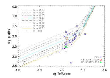
Figure 3: Spectroscopically determined log T_eff vs. log $g$ and evolutionary tracks for model masses $0.53\leq\rm{M/M_{\odot}}\leq 0.8$ and [M/H] $=-2.27$ by Cassisi et al. (2004). CS 30317-056 is shown as a green triangle, CS 22881-039 as a red square, and the RHB stars of Preston et al. (2006) as blue $\times$-es.

Figure 3 shows the Cassisi et al. (2004) evolutionary tracks in the log $T_{\rm eff}$ – log $g$ plane together with our spectroscopic values for CS 30317-056 and CS 22881-039. The Preston et al. (2006) RHB stars are shown for comparison; as seen, CS 30317-056 and CS 22881-039 fall well within the range covered by these stars (i.e. outside the instability strip ending at the fundamental red edge at log T${}_{eff}=3.80$).

5 Abundance Analysis

5.1 LTE abundances

The LTE abundances were generally obtained from equivalent widths (listed in online Table A), determined by fitting Gaussian profiles to observed lines from the lists of Hill et al. (2002). For this, we used the genetic algorithm fitline of François et al. (2003). Lines were disregarded if they were blended or very weak ($<0.5$ pm); in case of doubt, the Cayrel (1988) formula was used to assess the uncertainty of the equivalent width.

If the Gaussian fit seemed uncertain, the equivalent width was remeasured by direct integration in IRAF and checked with an LTE synthetic spectrum computed with turbospectrum (Alvarez & Plez 1998). If the two derived abundances differed significantly, the turbospectrum result was adopted. For a few elements, the abundance could only be determined from the synthetic spectrum fit.

We did not detect the Li I lines at 610.36 nm and 670.79 nm, even though the quality of the spectra was optimal in this region. The measured noise levels would allow to detect lines down to $\sim 4$ mÅ in equivalent width, which leads to the upper abundance limits for Li given in Table 4.

We have tried to measure the C abundance of CS 22881-039 and CS 30317-056 from a fit to the G band of the CH molecule. Since we found that $T_{\rm eff}$ and log $g$ did not change between the three blue spectra of CS 30317-056 (section 4), we coadded the spectra (correcting for the radial velocity variation) to improve the S/N ratio in the G-band region.

The LIFBASE program of Luque & Crosley (Luque 1996) was used to compute line positions and gf-values; excitation energies were taken from the line list of Jorgensen et al. (1996). The spectral regions free from contamination by atomic lines are indicated in the figure. Carbon is not detected, neither in CS 22881-039 nor in CS 30317-056, but the noise is large. For both stars the upper limit to the C abundance is $\rm log\leavevmode\nobreak\ \epsilon(C)=6.5$ (Fig. 4) or $\rm[C/H]\lesssim-2$.

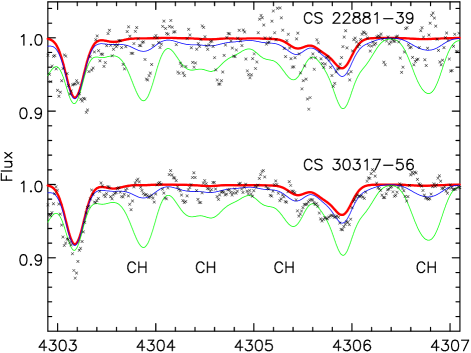
Figure 4: Synthetic spectrum fits to the CH band in CS 22881-039 and CS 30317-056. Crosses: observations; thick line: spectra computed with no carbon; thin lines: spectra computed for $\rm log\epsilon(C)=6.5$ and 7.2. The observed spectra are compatible with a complete absence of carbon; an upper limit to the abundance is $\rm log\leavevmode\nobreak\ \epsilon(C)\lesssim 6.5$.

We have also tried to measure the Na abundance in CS 22881-39 and CS 30317-56. In CS 30317-56 we observe a strong variation of the shape of the Na D lines with pulsation phase, $\phi$: At $\phi\approx 0.30$ the D lines are relatively narrow and symmetric, while they are broad and asymmetric at $\phi=0.13$. Only the first red spectrum (taken together with one of the blue spectra used to determine $T_{\rm eff}$ , log g, and $\rm\xi_{t}$) was applied to determine the Na abundance.

In CS 22881-39 the D lines are broad and asymmetric and unsuitable for an abundance determination. Since we have only one spectrum, we could not determine whether the asymmetry is due to shock waves in the atmosphere just before the steep rise to light maximum or to a blend by interstellar D lines.

The shape of the aluminium lines is very similar in the three blue spectra of CS 30317-56. Thus we have used the mean spectrum to fit the line profiles. (Since one of the Al lines is in the wing of the Balmer line $\rm H\epsilon$, it is better to determine the abundance from a synthetic spectrum fit). We find [Al/Fe]=-0.77 for CS 22881-39 and [Al/Fe]=-0.51 for CS 30317-56.

LTE abundances for the 16 elements O, Na, Mg, Al, Si, S, Ca, Sc, Ti, Cr, Mn, Fe, Co, Ni, Sr and Ba in CS 30317-056 and CS 22881-039 are listed in Table 4 together with the NLTE abundance corrections discussed in the following section. Errors of abundances based on only one line have been estimated from the uncertainty of the equivalent width. For an easier comparison with the other “First Stars” papers we have adopted the same (1D, LTE) solar reference abundances from Grevesse & Sauval (1998), which differ by typically only $\sim 0.1$ dex from the 3D+NLTE solar abundances by Asplund et al. (2009).

Table 4: LTE abundance ratios and adopted NLTE corrections for our two RR Lyr stars. $\sigma$ is the standard deviation and N the number of individual lines. ’ul’ indicates an upper limit, ’*’ a value derived from a turbospectrum fit, and a $\sim$ that the $\Delta_{\rm NLTE}$ value is a rough estimate or only valid for some lines.

Abundance	CS~22881-039	$\sigma$	N	$\Delta_{\rm NLTE}$	CS~30317-056	$\sigma$	N
log $\epsilon$ (Li)	$\sim$ 0.6	ul	1	–	$\sim$ 1.0	ul	1
[C/Fe]	0.69	ul	–	–	0.79	ul	–
[O/Fe]	–	–	–	-0.1	0.9	0.24	1
[Na/Fe]	-0.13	0.15	2	-0.2/-0.1	–	0.13	2
[Mg/Fe]	0.70	0.30	6	$\sim$0.05	0.48	0.15	6
[Al/Fe]	-0.74	0.05	2	+0.7	-0.66	0.15	2
[Si/Fe]	0.01	0.05	1	-0.05	0.05	0.05	1
[S/Fe]	–	–	–	-0.4	0.78	0.07	1
[Ca/Fe]	0.29	0.30	5	$\sim$0.19	0.4	0.13	6
[ScII/Fe II]	0.11	0.06	3	–	0.14	0.06	3
[TiI/Fe I]	0.38	0.25	1	–	0.63	0.16	6
[TiII/Fe II]	0.35	0.25	17	–	0.55	0.12	27
[Cr/Fe]	-0.32	0.12	4	+0.4	-0.18	0.05	5
[Mn/Fe]	-0.59	0.05	2	+0.6	-0.63	0.05	3
[Co/Fe]	0.14	0.14	2	$\sim$+0.6	0.27	0.06	2
[Ni/Fe]	-0.19	0.07	2	–	-0.13	0.05	3
[SrII/Fe II]	0.00	0.15	1	+0.6	0.03	0.10	2
[BaII/Fe II]	-0.62	0.09	1	$\sim$+0.15	-0.32	0.05	2

5.2 NLTE abundance correction

NLTE effects become important when the aim is not just to compare results for different stars, but to confront the data with supernova models, which are independent of our incomplete understanding of stellar atmospheres.

NLTE calculations in the literature generally apply to either dwarfs or giants. We have therefore calculated NLTE abundance corrections $\Delta_{\rm NLTE}$  for O and Mg for our stars and estimated other corrections from studies of dwarfs and giants. These corrections are discussed below and listed for all lines in online Table A.

Oxygen.

NLTE corrections for the O I triplet were computed using the Kiel code (Steenbock & Holweger 1984) and MARCS model atmospheres. The O model atom is from Paunzen et al. (1999). The cross-sections for inelastic H I collisions were computed according to Drawin (1969). Setting the scaling factor for these cross-sections (S_H) to $0$ and $1$, respectively, we obtain a correction of $-0.1$ dex in both cases.

When we compare these corrections to the more recent values estimated from Fabbian et al. (2009) we find that our corrections are lower. Fabbian et al. (2009) estimated NLTE corrections for RR Lyr stars 500 K warmer than our stars and obtained values of -0.5 and -0.35 for S_H = 0 and 1, respectively. Their Fig. 8 shows how the NLTE corrections for oxygen vary with temperature and gravity and demonstrates that temperature has a much larger influence on the corrections than gravity; a difference in $\Delta_{NLTE}$ for S${}_{H}=0$ of -0.4 dex corresponds to a difference of +1000 K in temperature. The warmer metal-poor stars yield a correction of -0.5 dex, compared to -0.1 dex for the cooler metal-poor turn-off stars. This would yield a correction of approximately -0.3 dex for our stars with S_H = 0.

$\alpha$-elements.

For magnesium we use precise NLTE corrections kindly calculated by S. Andrievsky, using the MULTI and SYNTHV codes described in Andrievsky et al. (2010), taking fine structure of the 3p 3P* levels into account, and adopting our oscillator strengths. The accurate results for individual lines in our two stars are listed in the online Table A. $\Delta_{\rm NLTE}$ varies from 0.0 to 0.17 dex for the various Mg lines; an average value is $\sim$0.05 dex.

For Silicon, $\Delta_{\rm NLTE}$ is small, typically from 0.0 to +0.25 dex, according to Shi et al. (2009), who mainly consider dwarf stars; for the 390.5 nm line we adopt a mean value of 0.05 dex from the 14 stars of their Table 2. Preston et al. (2006) noted that silicon abundances for stars hotter than 5800 K decrease with increasing temperature and should thus not be trusted as chemical tracers. The temperatures of our stars are close to 5800 K, so we still trust our values (in LTE and NLTE), but note that a somewhat larger uncertainty ($\pm$ 0.1 dex) is probably in order.

Sulphur abundances from the 921.2 nm line need a larger correction. With (S${}_{\rm H}=1$), $\Delta_{\rm NLTE}$ = -0.4 dex is interpolated between the two sets of stellar parameters ($T_{\rm eff}$ /log $g$ /[Fe/H] = 5500/2.0/-2.0 and 6500/2.0/-3.0) in Takeda et al. (2005).

For four of our nine Ca lines, $\Delta_{\rm NLTE}$ has been taken from Mashonkina et al. (2007), who use a scaling factor of S${}_{H}=0.1$. The individual corrections are listed in Table A and an average value in Table 4.

No NLTE corrections currently exist for Ti.

Odd-$Z$ elements: Na, Al, Sc.

We estimate $\Delta_{\rm NLTE}$ = -0.2 and -0.1 dex for the Na D1 and D2 lines in our RR Lyr stars, based on the calculations of (Andrievsky et al. 2007), who applied the same codes and methods as described for Mg above and Al below. For Al, we estimate $\Delta_{\rm NLTE}$ = 0.7 dex for Al from Andrievsky et al. (2008), using a scale factor of 0.1 in the Drawin (1969) formula.

No $\Delta_{\rm NLTE}$ values for Sc in metal-poor stars are available yet. Zhang et al. (2008) suggest a correction of 0.3 dex for the Sun (an average for the three lines seen in our RR Lyr stars). Since we are dealing with Sc II, one might expect to get small NLTE corrections. However, due to the very different stellar parameters of our RR Lyr stars and the Sun and the strong dependence of the Sc abundance on microturbulence, we choose to not apply their $\Delta_{\rm NLTE}$ value to our stars.

Si-burning elements: Cr, Mn and Co.

NLTE abundance corrections for Mn, and Co were taken from Bergemann et al. (2010), Bergemann & Gehren (2008), and Bergemann et al. (2009), respectively. The Cr correction is estimated to be around 0.4 dex (M. Bergemann, priv. comm.).

Neutron-capture elements: Sr, Ba.

NLTE corrections for Sr in EMP stars are available from Mashonkina & Gehren (2001), who find $\Delta_{\rm NLTE}$ = 0.6 dex for stars of similar atmospheric parameters as ours, but do not list the lines used in this value. The correction is quite sensitive to the stellar parameters (Belyakova & Mashonkina 1997; Mashonkina & Gehren 2001), but the above value should be a good estimate for our stars.

$\Delta_{\rm NLTE}$ for Ba is given by Andrievsky et al. (2009) for the three lines at 455.4 nm (around 0.15 dex, 585.3 nm, and 649.6 nm. Thus, only the resonance line (455.4 nm) can be corrected in our spectrum of CS 30317-056 and none in CS22881-039, so we prefer to retain the uncorrected LTE Ba abundances in both stars.

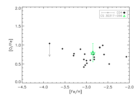
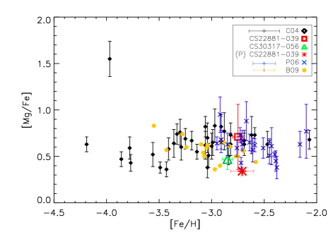
Figure 5: Left: NLTE values of [O/Fe] for our RR Lyr stars compared to the giants from Cayrel et al. (2004). Right: [Mg/Fe], corrected for NLTE, compared to EMP giants (Cayrel et al. 2004), dwarfs (Bonifacio et al. 2009), as well as the RHB stars from (Preston et al. 2006), all have been corrected for NLTE effects by applying corrections from Andrievsky et al. (2010). Results for CS 22881-039 are shown as a red square (this paper) and asterisk (Preston et al. 2006); other symbols as in Fig. 2.

6 Results

In this section we compare the abundances for our two RR Lyr stars with the earlier results for EMP giants and dwarfs Cayrel et al. (2004); François et al. (2007); Bonifacio et al. (2009), and RHB stars (Preston et al. 2006). Systematic differences in abundance scales between our results and the former should be minimal, because the observations and reductions were carried out in exactly the same way. Larger differences from the results of Preston et al. (2006) might be expected, since different observational approaches, model atmospheres, codes, and methods were used to determine the stellar parameters and abundances. Still, Preston et al. (2006) find that differences in individual elemental abundances computed with MARCS or ATLAS model atmospheres should be less than $0.05$ dex.

The abundance ratios relative to Fe are listed in Table 4 and shown graphically in the following (see e.g. Fig. 5, 7, 8 and 9). All abundance ratios shown were obtained assuming LTE, except when explicitly noted as corrected for NLTE effects. Note that NLTE effects in Fe might offset all these abundances ratios by a small amount. This offset might be as large as 0.2 dex (Mashonkina et al. 2010) but these corrections still need inclusion of many high energy levels to predict accurate abundance corrections. Generally, the figures show an abundance y-range of 2 dex, except for O, Sr and Ba. The two exceptional stars CS 22949-037 (Cayrel et al. 2004) and CS 29527-15 (Bonifacio et al. 2009) have been omitted in the comparisons. Overall, the detailed chemical composition of our two RR Lyr stars does not deviate significantly from the well-known mean trends for “normal” EMP giant and dwarf stars; we comment on individual element groups below.

The element abundances derived from the three spectra listed in Table 3 are very similar and yield very homogeneous abundances (the differences in abundances from the individual spectra are $\sim$ 0.05 dex - per element). Hence, the abundances are stable during the different pulsation phases (as noted in Kolenberg et al. (2010)), and should therefore be considered trustworthy as chemical tracers. Furthermore, the coadded spectra yield abundances agreeing within 0.05 dex with those obtained from the single spectra, except for a few elements, where the difference is around 0.1 dex.

6.1 Lithium

As expected, Li is not observed in our RR Lyr stars. During the evolution of the star along the RGB, the increasingly deep mixing has filled the external layers with the matter of deep, hot layers where lithium has been destroyed by proton fusion.

6.2 The $\alpha$-Elements

As in other EMP stars, we find [$\alpha$/Fe] $>0$ in our targets, with relatively small dispersion. We discuss the individual elements below.

Oxygen
O was only detected in CS 30317-056. Its abundance was determined from the O I triplet at 777.194 nm, which is affected by NLTE, while the O abundance for giant stars in Cayrel et al. (2004) were based on the forbidden [O I] line at 630 nm, which is insensitive to NLTE effects, but may be affected by 3D effects. However the O I 3D effects remain small for giants (Collet et al. 2006). As Fig. 5 shows, especially the corrected value of [O/Fe] in CS 30317-056 (Sect. 5.2) agrees well with the mean value for EMP giants found by Cayrel et al. (2004) without regard to 3D effects.

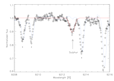
Figure 6: The observed spectrum of CS 30317-056 around the S line 921.3 nm (open diamonds). The dotted blue line shows the spectrum of a fast-rotating star with mainly telluric lines (indicated by ’*’). This confirms that the S line is indeed stellar and not telluric. The solid red line is an LTE synthetic spectrum fit to the S line, which confirms the abundance we obtain from direct integration.

Mg, Si, S, Ca, and Ti
Our Mg abundances are based on six lines in both stars, In CS 22881-39 the strong magnesium lines are asymmetric, which could indicate strong velocity fields inside the atmosphere (the star has been observed just before the sudden rise in luminosity). As a consequence, the Mg abundance deduced from a static model atmosphere cannot be completely reliable.

Small positive NLTE corrections have been applied to all Mg abundances in Fig. 5. For our RR Lyr stars (see Table 4) they were calculated specifically for this study (Sect. 5.2); for the Preston et al. (2006) HB stars we estimate $\Delta_{\rm NLTE}$ = 0.2 – $0.3$ dex, depending on the stellar parameters. This correction may be overestimated, since we found a much smaller value when getting the exact calculations compared to estimating the correction based on Andrievsky et al. (2010).

Our LTE abundances of Si are based on the single line at 390.5 nm and exhibit large scatter, as also found by Preston et al. (2006). Our abundances are somewhat lower than those for giants by Cayrel et al. (2004), but agree with those for turnoff stars by Bonifacio et al. (2009). This difference may be linked to the temperature dependence noted by Preston et al. (2006), who recommended to only trust abundances for stars with temperatures below 5800 K. Our stars are close to this limit, so we expect our Si abundances to be fairly reliable. (The difference between the dwarfs and giants could be due to NLTE effects).

Sulphur is an interesting element, because it has so far only been detected in a few EMP stars (e.g., CS 29497-030, Sivarani et al. (2004)). Here it is measurable in CS 30317-056 only (see Fig. 6). An LTE analysis of the strong triplet at 921.286 nm yields [S/Fe] = 0.78 dex, above the mean value by Nissen et al. (2007), but in agreement with Caffau et al. (2005) and other sources listed in Nissen et al. (2007). Using the value of $\Delta_{\rm NLTE}$ = -0.4 dex from Takeda et al. (2005), the agreement is essentially perfect.

Our [Ca/Fe] ratios from six Ca I lines, whether derived in LTE or NLTE, agree within the errors with Preston et al. (2006) and Cayrel et al. (2004). The LTE abundance of Ti in CS 22881-039 match the Ti abundances for giants (Cayrel et al. 2004), while that for CS 30317-056 matches the higher values for dwarfs by Bonifacio et al. (2009); both are in the range found for EMP RHB stars by Preston et al. (2006). The Ti I and Ti II LTE abundances agree well, within 0.08 dex, supporting the gravity derived from the ionisation balance of Fe.

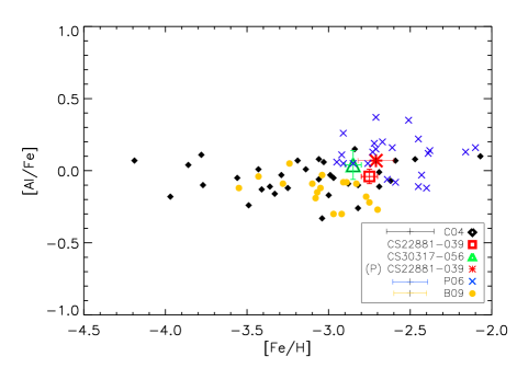
Figure 7: [Al/Fe] for our RR Lyr stars and the RHB stars by Preston et al. (2006), as well as for giants Cayrel et al. (2004), all corrected for NLTE; symbols as in Fig. 5.

6.3 The Odd-Z Elements Na, Al, and Sc

Na and Al abundances derived from the resonance lines of the neutral atoms are very sensitive to NLTE effects. According to Cayrel et al. (2004) and Bonifacio et al. (2009), $\Delta_{\rm NLTE}$ is of the order of $-0.2/-0.1$ dex for Na and $+0.70$ dex for Al. Fig. 7 compares our NLTE results for Al with those from the earlier study by (Andrievsky et al. 2008). From the stellar parameters and the calculations of Andrievsky et al. (2008), we estimate $\Delta_{\rm NLTE}$ for the Preston et al. (2006) RHB stars to be 0.8 – 1.0 dex for Al, depending on the stellar parameters.

The values of [Sc/Fe] for both RR Lyr stars are well within the range seen in Cayrel et al. (2004). The observed trend of [Sc/Fe] is flat, with a scatter of only $0.12$ dex (Cayrel et al. 2004).

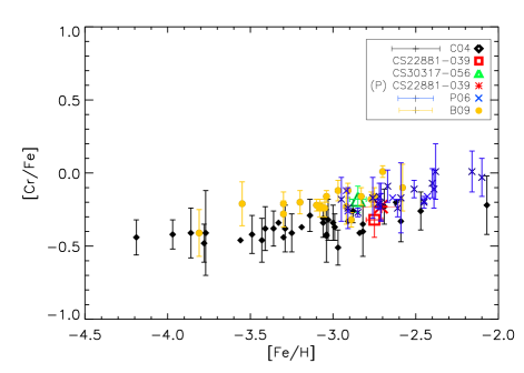
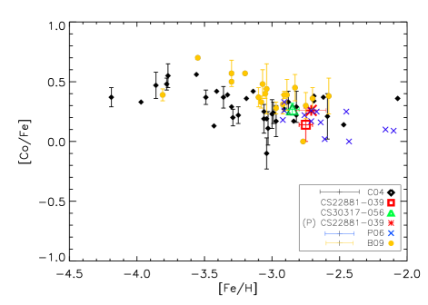
Figure 8: [Cr/Fe] and [Co/Fe] vs. [Fe/H] (symbols as in Fig. 5), all derived in LTE. The RR Lyr stars agree well with the results of Preston et al. (2006), Cayrel et al. (2004) and Bonifacio et al. (2009).

6.4 Iron-peak Elements

To facilitate comparison with theoretical yields from supernova models, we discuss the two subgroups of the iron-peak elements separately. We note that iron itself, which is used as the reference element, may be affected by NLTE effects (Mashonkina et al. 2010), which would shift all the abundance ratios discussed in the following slightly up or down by a fixed amount. Most of the iron-peak abundance ratios are extremely tightly defined – so tightly, in fact, that interpretations of the slopes (notably that of the [Cr/Fe] relation) in terms of metallicity-dependent supernova masses appear implausible. Cayrel et al. (2004) discussed residual NLTE effects for the abundance trends as a possible alternative, which seems to be confirmed by the diverging abundances from Cr I and Cr II lines found by Bonifacio et al. (2009).

Incomplete Silicon Burning Elements: Cr and Mn
Our Cr abundances are based on three Cr I lines, and the Mn abundance on the three Mn I resonance lines near $403$ nm (see Table A). Since the Mn lines are weak in these stars, no special treatment of the hyperfine structure was necessary. No lines of ionised Cr and Mn were detected in our RR Lyr stars.

The LTE abundances of Cr and Mn for our two RR Lyr stars agree within 0.1 dex with those by Preston et al. (2006), Cayrel et al. (2004), and Bonifacio et al. (2009) (Fig. 8) – better than the combined errors. Bonifacio et al. (2009) suggest that NLTE effects in Cr may be significant in metal-poor stars; if so, [Cr/Fe] in this metallicity range should be $\sim 0.1$.

Complete Silicon Burning Elements: Co and Ni
Our Co and Ni abundances are based on two neutral lines each in both stars. Within our estimated error, we find good agreement between our LTE abundances and those of the EMP stars of Cayrel et al. (2004), Bonifacio et al. (2009), and Preston et al. (2006) (Co only). However, we note that NLTE effects for Co in our RR Lyr stars are large and positive (Table 4).

6.5 Neutron-Capture Elements: Sr and Ba

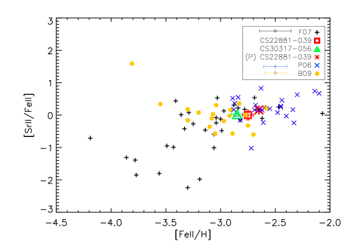
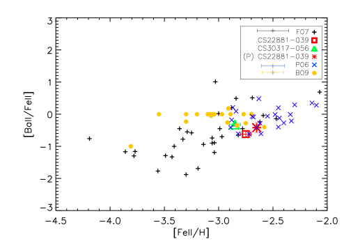
Figure 9: [Sr/Fe] and [Ba/Fe] in EMP stars, assuming LTE (symbols as in Fig. 5; note the change in vertical scale here). Our RR Lyr stars agree well with the previous relations for giants, dwarfs and RHB stars (Cayrel et al. 2004; Bonifacio et al. 2009; Preston et al. 2006).

Sr and Ba are the only neutron-capture elements detected in our RR Lyr stars. Their abundances are determined from the resonance lines and hence subject to NLTE effects. However, as noted above, consistent NLTE corrections for Ba in our stars are not available in the literature, so we have chosen not to correct our [Ba/Fe] ratios for NLTE.

Both [Sr/Fe] and [Ba/Fe] show huge scatter below [Fe/H]$\sim-3$, far in excess of observational errors (Primas et al. 1994; McWilliam et al. 1995; François et al. 2007) – see Fig. 9. Taking this into account, our results for CS 22881-039 and CS 30317-056 (both corrected and uncorrected) agree within the combined errors with the abundances found by Preston et al. (2006) and For & Sneden (2010) for the RHB stars and also with the concordant results for EMP dwarfs and giants discussed by Bonifacio et al. (2009).

7 Supernova Models and Yields

Having verified that our RR Lyr stars can be included in general samples of EMP stars, we proceed to compare the derived stellar abundances in our EMP RR Lyr stars with the supernova model yields of Limongi et al. (2000), Kobayashi et al. (2006), Tominaga et al. (2007) and Izutani et al. (2009). It is generally believed that SNe of Type Ia did not contribute significantly to the composition of the EMP stars, so only models of core-collapse SNe with massive progenitor stars need to be considered here.

These models are characterised by a number of parameters, such as the mass of the progenitor, the explosion energy, the peak temperature, the mass cut, the electron density in the proto-neutron star, $Y_{e}$ , the amount of fallback and/or mixing, and the degree of anisotropy, including any pre-explosion jets. Variations in these parameters are manifested in characteristic changes in the predicted element ratios, so the observed abundance patterns can be used to constrain the values of these parameters. For such comparisons, NLTE corrected abundances must of course be used whenever available – see Table 4.

Even EMP stars are presumably the result of more than one SN explosion, so the assumed properties of the progenitor population – notably the IMF – enter implicitly into the comparison of models vs. observations. Only models assuming a Salpeter IMF have been chosen here in order to compare models on an equal basis without introducing differences due to changes in the IMF.

A Salpeter IMF is the standard assumption in supernova and galactic chemical evolution models. Top-heavy IMF’s have been tested as well by Ballero et al. (2006); Matteucci (2007). Both studies find that if the presumed POP III stars more massive than 100 M_⊙ resulting in Pair Instability SNe (PISNe) with yields showing a strong odd/even effect, the overall impact on the early ISM is negligible. Only if these very massive stars kept forming for generations would one see an imprint of them, and this is not detectable in the observations. In fact, Ballero et al. (2006) find that a constant or slightly varying ISM yields the best results when comparing to observations of metal-poor stars.

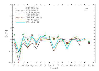
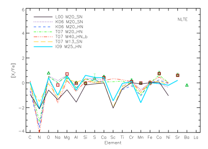
Figure 10: Observed abundance ratios in our RR Lyr stars from Table 4 (symbols as in Fig. 5)vs. predicted yields for models of super- and hypernovae (HN) by: Limongi et al. (2000) (full black line), Kobayashi et al. (2006) (dotted: SN; dashed: HN), Tominaga et al. (2007) (dot-dashed and triple-dot-dashed: 20 and 40 $M_{\odot}$ HN; long-dashed: 13 $M_{\odot}$ SN) and Izutani et al. (2009) 25 $M_{\odot}$ HN; thick blue solid line.

Fig. 10 shows that the various model yields differ most strongly for certain elements, which therefore become the most important diagnostics of the different model features. These elements are, notably, Na, Mg, Al, Sc, Mn and the neutron-capture element Sr. Lai et al. (2008) found that Si, Ti, and Cr exhibit clear trends with stellar parameters such as the temperature, so these elements are less useful in this context.

Only models that provide the fit to the abundances observed are included in Fig. 10. Models of the putative, extremely massive PISNe (Heger & Woosley 2002b; Depagne et al. 2002)) predict a much larger odd-even effect than observed. These very heavy SN were therefore not considered here.

7.1 The $\alpha$-elements

The $\alpha$-elements are generally formed in massive progenitor stars already before the SN explosion and thus bring information on the nature of the first stellar population(s). E.g., O (and C) are primarily produced in core helium burning in massive stars, O also during Ne burning, and Mg is produced in shell carbon burning. The paucity of iron formed by SNe II relative to the Solar composition causes the familiar over-abundance of the $\alpha$-elements, typically $\sim$0.3 dex, in metal-poor stars (see Table 4).

Supernova models Heger & Woosley (2002a); Kobayashi et al. (2006) indicate that larger yields of even-Z elements, also seen as a large odd-even effect, correspond to a larger (total or at least envelope) mass of the progenitor star. However, the magnitude of the observed odd-even effect depends heavily on a few relatively large NLTE abundance corrections, especially that for Al, so computing or estimating $\Delta_{\rm NLTE}$ correctly is of direct importance for the conclusions that can be drawn on the mass of the progenitor stars.

7.2 The Odd-Z Elements

The odd-Z elements are generally under-abundant by $\sim$0.2 dex relative to the Sun. Na and Al are produced in the progenitor before the SN explosion, but Sc is produced in explosive O and Si burning, and also in Ne burning (Woosley & Weaver 1995), hence in the SN itself.

The Sc abundance appears to be the best diagnostic of the explosive energy of the SN: The high (=near-Solar) [Sc/Fe], and to a lesser degree [Ti/Fe], ratios suggest that very energetic SNe (Hypernovae) were the progenitors of the EMP stars we observe today. We note, however, that $\Delta_{\rm NLTE}$ for Sc has not yet been computed, and a large negative value would affect this conclusion.

Moreover, according to Izutani et al. (2009), high Sc and Ti are tracers of a high $Y_{e}$ to an even larger extent than a high explosion energy. A high-energy explosion is still required, but it is not the primary cause of a large production of Sc and the neutron capture elements. Models with (artificially) high values of $Y_{e}$ (Izutani et al. 2009; Tominaga et al. 2007) and low-density modifications caused by, e.g., jet-like explosions and fallback (Tominaga et al. 2007) fit the abundance patterns of EMP stars better, as indicated by the relatively large amounts of Sc and Sr. The caveat about NLTE effects should be kept in mind, however.

7.3 Silicon Burning Elements

Among the iron-peak elements, Cr and Mn are produced by incomplete silicon burning and Co, Ni and Zn in complete silicon burning during supernova explosions. Incomplete silicon burning occurs at temperatures of $4\cdot 10^{9}$K $<T_{peak}<5\cdot 10^{9}$K (Nomoto et al. 2005), complete silicon burning at temperatures above $5\cdot 10^{9}$K. The observed high abundances of the complete Si burning elements indicate that the peak temperatures reached by the progenitor SNe was indeed high. At higher metallicities than discussed here, the production of Ni (and Fe) is, of course, dominated by the entirely different processes in SNe Ia.

7.4 Neutron-capture Elements

At Solar and moderately low metallicity, the abundances of Sr and Ba are dominated by the s-process (Arlandini et al. 1999). In EMP stars, however, the neutron-capture elements should all be due to the r-process (Spite & Spite 1978; Truran 1988; François et al. 2007), so observations of Sr and Ba in EMP stars should provide useful constraints on the site of the $r$-process (Heger & Woosley 2002a).

In past decades, core-collapse supernovae have been considered the most promising astrophysical site for the r-process, but this scenario is facing difficulties (e.g. Wanajo et al. 2010), and there is presently no consensus on the site of the $r$-process(es).

Unfortunately, we only have NLTE-corrected abundances for Sr, and $\Delta_{\rm NLTE}$ for Ba might be appreciable (see Sect. 5.2), so our present ability to place strong constraints is limited. Constraints on $Y_{e}$ could be derived from abundances of light neutron-capture elements, i.e. elements in the range $38<Z<48$. Slight enhancements of Sc (and Ti) are consistent both with a high $Y_{e}$ or a jet-like explosion (cf. the good fit of the Tominaga et al. (2007) models to the data in Fig. 10).

8 $T_{\rm eff}$ at the RR Lyr-RHB Boundary

One of the aims of the paper of Preston et al. (2006) was to determine the temperature of the red edge of the RR Lyr instability strip (the “fundamental red edge”: FRE in the pulsation theory). Horizontal branch stars cooler than the FRE do not pulsate, because at this temperature the onset of convection disrupts the pulsation mechanism. This limit is difficult to predict theoretically, however, because such a prediction requires a very good understanding of the role of convection in RR Lyr pulsations. Preston et al. (2006) estimated the FRE temperature by comparing the temperature distribution of RR Lyr stars and RHB stars in globular clusters and in field stars. He found that in both cases no RR Lyr star was found below log $T_{\rm eff}$ = 3.80. Accordingly, he adopted for $\rm[Fe/H]<-2$, $\rm logT_{eff}(FRE)=3.80\pm 0.01$ or $\rm T_{eff}(FRE)=6300\pm 150\leavevmode\nobreak\ K$.

CS 22881-039 and CS 30317-056 are both significantly cooler than the FRE as defined by Preston et al. (2006); nevertheless, they are photometric variables with light curves and periods like those of RR Lyr stars. Nemec (2004) found three RR Lyr below this limit in NGC5053 ($\rm[Fe/H]\sim-2.30$), and it is interesting that the photometric amplitude of these stars is small ($\rm<0.6mag$). In a recent paper, For & Sneden (2010) compared the temperature distributions of non-variable HB stars and RR Lyr stars and estimated the temperature of the FRE in the interval $\rm-0.8\lesssim[Fe/H]\lesssim-2.5$ be about 5900 K, in good agreement with our result. Hence, at the lowest metallicities the temperature of the FRE is probably lower than estimated by Preston et al. (2006); ${\rm T_{eff}(FRE)}\approx$ 5900 K would be probably a better estimate. Moreover, the RR Lyr stars found very close to the FRE seem to have smaller photometric amplitudes than typical RRab.

9 Conclusions

Our detailed analysis of two EMP RR Lyr stars from high-resolution VLT/UVES spectra have yielded abundances for 16 elements, which agree very well (generally within $\leq 0.2$ dex) with those by Cayrel et al. (2004), Bonifacio et al. (2009), and Preston et al. (2006), for giants, dwarfs, and RHB stars, respectively. Due to the homogeneity of the stellar abundances from the individual spectra, despite the pulsation, our RR Lyr stars can be used as chemical tracers as well as non-variable RHB stars.

The temperature of the fundamental red edge of the instability strip is probably lower at low metallicity than obtained by Preston et al. (2006); our results suggest a value of $T_{\rm eff}(FRE)\approx 5900\leavevmode\nobreak\ K$, in agreement with For & Sneden (2010).

Our comparison of the abundance patterns of well-studied EMP stars with supernova yields from the models of Tominaga et al. (2007); Nomoto et al. (2005) with varying $Y_{e}$, mass cut, mixing, and fallback indicates that supernovae with relatively large masses (up to 40 M_⊙) and large explosion energies provide the best overall match to the observations. Including the NLTE corrections leaves much the same overall picture of the predecessor SNe, but lowers the estimate of the progenitor mass.

Overall, among current models, the 40 M_⊙ HN model by Tominaga et al. (2007) seems to provide the best fit to our LTE abundance trends, even though it is not straightforward to constrain the mass and energy of the previous generation of SNe when varying some parameters such as $Y_{e}$ while keeping others fixed. On the other hand, when we compare the NLTE corrected abundances to the same models, the 25 $M_{\odot}$ hypernova model by Izutani et al. (2009) appears to give the best fit (or the 20 $M_{\odot}$ HN model by Tominaga et al. (2007)) , because the NLTE abundances of such elements as Na, Al, S, Sc, Ti and the iron-peak elements differ from the predictions of the 40 $M_{\odot}$ HN model. Hence, good determination of the NLTE effects for these elements are particularly important in comparisons with SN models. Sc is a key element in such work, and a good NLTE analysis of Sc is an urgent priority. Zn is another very important diagnostic element, but is not observable in such hot EMP stars as those discussed here.

[x]llllllll Equivalent widths and abundances of iron lines

CS 30317-056 CS 22881-039
$\lambda$ $\chi$ log gf Ref. EW A(Fe) EW A(Fe)
nm eV pm dex pm dex

continued.

CS 30317-056 CS 22881-039
$\lambda$ $\chi$ log gf Ref. EW A(Fe) EW A(Fe)
nm eV pm dex pm dex

Fe i
337.0783 2.69 $-0.266$ BWL – – – –
339.9333 2.20 $-0.622$ BWL 1.54 3.57 – –
340.1519 0.92 $-2.059$ BWL 1.37 3.54 – –
340.7460 2.18 $-0.020$ BWL 3.68 3.52 1.76 3.96
341.3132 2.20 $-0.404$ BWL 2.03 3.51 – –
341.7841 2.22 $-0.676$ BWL – ——
341.8507 2.22 $-0.761$ BWL 1.12 3.57 —-
342.4284 2.18 $-0.703$ BWL – – – –
342.5010 3.05 $-0.500$ BWL – ——
342.6383 0.99 $-1.909$ BWL – ——
342.7119 2.18 $-0.098$ BWL 3.48 3.54 —-
342.8193 2.20 $-0.822$ BWL 0.82 3.44 —-
344.0606 0.00 $-0.673$ BWL 10.11 3.60 7.22 4.08
344.0989 0.05 $-0.958$ BWL 8.83 3.64 6.00 4.03
344.3876 0.09 $-1.374$ BWL 7.93 3.83 3.79 3.90
344.5149 2.20 $-0.535$ BWL 2.22 3.69 – –
345.0328 2.22 $0.902$ BWL – – – –
345.2275 0.96 $-1.919$ BWL 1.65 3.54 – –
347.5450 0.09 $-1.054$ BWL 8.53 3.67 4.94 3.85
347.6702 0.12 $-1.507$ BWL 7.22 3.76 4.07 4.12
348.5340 2.20 $-1.149$ BWL – – – –
349.0574 0.05 $-1.105$ BWL 9.11 3.84 4.96 3.87
349.7841 0.11 $-1.549$ BWL 7.07 3.73 2.62 3.81
352.1261 0.92 $-0.988$ BWL 6.16 3.74 2.15 3.87
353.3198 2.88 $-0.112$ BWL – – – –
353.6556 2.88 $+0.115$ BWL 1.71 3.60 – –
354.1083 2.85 $+0.252$ BWL – – – –
354.2076 2.87 $+0.207$ BWL 2.09 3.61 – –
355.3739 3.57 $+0.269$ BWL 1.07 3.95 – –
355.4118 0.96 $-2.206$ BWL 1.80 3.86 – –
355.4925 2.83 $+0.538$ BWL 2.75 3.42 – –
355.6878 2.85 $-0.040$ FMW 2.18 3.87 – –
356.5379 0.96 $-0.133$ BWL 7.86 3.43 4.90 3.72
358.1193 0.86 $+0.406$ FMW 11.12 3.49 7.43 3.81
358.4659 2.69 $-0.157$ BWL 1.57 3.62 – –
358.5319 0.96 $-0.802$ BWL 6.79 3.77 2.60 3.84
358.5705 0.92 $-1.187$ FMW 5.45 3.72 – –
358.6113 3.24 $+0.173$ BWL 1.18 3.73 – –
358.6985 0.99 $-0.796$ BWL – – – –
358.9105 0.86 $-2.115$ FMW 1.96 3.71 – –
360.3204 2.69 $-0.256$ BWL 1.11 3.54 – –
360.6679 2.69 $+0.323$ BWL 3.55 3.66 – –
360.8859 1.01 $-0.100$ FMW 8.36 3.57 4.61 3.66
361.0159 2.81 $+0.176$ BWL 2.06 3.57 – –
361.7786 3.02 $-0.029$ BWL+BK 1.39 3.78 – –
361.8768 0.99 $-0.003$ BWL 8.85 3.58 5.35 3.73
362.2003 2.76 $-0.150$ BWL 2.09 3.85 – –
362.3186 2.40 $-0.767$ BWL 1.24 3.80 – –
363.8296 2.76 $-0.375$ BWL – – – –
364.0389 2.73 $-0.107$ BWL 1.46 3.57 – –
364.7843 0.92 $-0.194$ FMW 8.45 3.52 5.66 3.76
380.5343 3.30 $0.312$ BWL – – – –
380.6696 3.27 $+0.017$ BWL – – – –
380.7537 2.22 $-0.992$ BWL – – – –
381.5840 1.49 $+0.237$ BWL 8.56 3.63 5.67 3.82
381.6340 2.20 $-1.196$ BWL 0.68 3.65 – –
382.0425 0.86 $+0.119$ FMW 10.82 3.58 7.92 3.94
382.1178 3.27 $+0.198$ BWL 1.14 3.66 – –
382.5881 0.92 $-0.037$ FMW 9.89 3.62 – –
382.7823 1.56 $+0.062$ FMW 7.49 3.60 – –
384.0438 0.99 $-0.506$ FMW – – – –
384.1048 1.61 $-0.045$ BWL – – – –
384.3257 3.05 $-0.241$ BWL – – – –
384.9967 1.01 $-0.871$ FMW 6.64 3.71 3.34 3.99
385.0818 0.99 $-1.734$ FMW 3.21 3.72 0.55 3.87
385.2573 2.18 $-1.185$ BWL .70 3.63 – –
385.6372 0.05 $-1.286$ FMW 9.26 3.85 5.45 3.96
385.9213 2.40 $-0.749$ BWL 1.10 3.66 – –
385.9911 0.00 $-0.710$ FMW 11.39 3.66 8.22 4.07
386.5523 1.01 $-0.982$ FMW 6.30 3.72 2.91 4.01
386.7216 3.02 $-0.451$ BWL 0.73 3.82 – –
387.2501 0.99 $-0.928$ FMW 6.39 3.67 3.08 3.97
387.3761 2.43 $-0.876$ BWL – – – –
387.8018 0.96 $-0.914$ FMW 6.90 3.76 – –
388.6282 0.05 $-1.076$ FMW – – – –
388.7048 0.91 $-1.144$ FMW – – – –
389.5656 0.11 $-1.670$ FMW 8.06 3.94 – –
389.9707 0.09 $-1.531$ FMW 8.47 3.90 – –
390.2946 1.56 $-0.466$ FMW 6.01 3.71 3.49 4.11
390.6480 0.11 $-2.243$ FMW 6.00 3.91 1.41 4.01
391.7181 0.99 $-2.155$ FMW 1.76 3.76 – –
392.0258 0.12 $-1.746$ FMW 7.62 3.89 3.27 4.02
392.7920 0.11 $-1.522$ BWL 8.70 3.97 4.32 4.00
394.0878 0.96 $-2.600$ FMW 1.14 3.94 – –
394.9953 2.18 $-1.251$ BWL 0.96 3.84 – –
395.6677 2.69 $-0.429$ BWL 1.31 3.73 – –
397.7741 2.20 $-1.119$ BWL 0.96 3.72 – –
399.7392 2.73 $-0.479$ BWL 1.03 3.69 0.72 4.32
400.5242 1.56 $-0.610$ FMW 5.10 3.61 2.27 3.97
400.9713 2.22 $-1.252$ BWL 0.73 3.75 – –
401.4531 3.05 $-0.587$ BWL 0.65 3.92 – –
402.1867 2.76 $-0.729$ BWL 0.61 3.72 – –
404.5812 1.49 $+0.280$ FMW 8.88 3.61 6.84 4.02
406.3594 1.56 $+0.062$ BWL 7.92 3.65 5.49 3.98
407.1738 1.61 $-0.022$ FMW 7.36 3.64 4.80 3.97
413.2058 1.61 $-0.675$ BWL 4.88 3.66 1.81 3.94
413.4678 2.83 $-0.649$ BWL 0.63 3.72 – –
414.3415 3.05 $-0.204$ BWL 0.75 3.59 – –
414.3868 1.56 $-0.511$ BWL 5.63 3.62 2.59 3.93
418.1755 2.83 $-0.371$ BWL 1.43 3.84 – –
418.7039 2.45 $-0.548$ FMW 1.36 3.58 – –
418.7795 2.42 $-0.554$ FMW 1.56 3.63 – –
419.1431 2.47 $-0.666$ BWL 1.15 3.63 – –
419.8304 2.40 $-0.719$ FMW 1.63 3.79 – –
419.9095 3.05 $+0.155$ BWL 1.94 3.71 – –
420.2029 1.49 $-0.708$ FMW 5.68 3.74 – –
421.0344 2.48 $-0.928$ BWL 0.82 3.74 – –
421.6184 0.00 $-3.356$ FMW 1.80 3.84 – –
421.9360 3.57 $+0.000$ BWL 0.55 3.80 – –
422.2213 2.45 $-0.967$ FMW 1.18 3.92 – –
422.7427 3.33 $+0.266$ BWL 1.08 3.60 – –
423.3603 2.48 $-0.604$ FMW 1.44 3.69 – –
423.5937 2.42 $-0.341$ FMW 2.21 3.60 – –
425.0119 2.47 $-0.405$ FMW 1.98 3.65 – –
425.0787 1.56 $-0.714$ BWL 5.02 3.66 – –
426.0474 2.40 $+0.109$ BWL+BK 4.18 3.56 – –
427.1154 2.45 $-0.349$ FMW 2.41 3.68 – –
427.1761 1.49 $-0.164$ FMW 7.87 3.74 – –
428.2403 2.18 $-0.779$ BWL 1.69 3.62 – –
429.9235 2.42 $-0.405$ BWL – – 0.25 3.46
432.5762 1.61 $+0.006$ BWL 7.77 3.67 – –
435.2735 2.22 $-1.287$ BWL 0.83 3.81 – –
437.5930 0.00 $-3.031$ FMW 3.17 3.85 – –
438.3545 1.49 $+0.200$ FMW 9.00 3.63 – –
440.4750 1.56 $-0.142$ FMW 7.32 3.63 – –
441.5123 1.61 $-0.615$ FMW 5.45 3.69 – –
442.7310 0.05 $-2.924$ BWL 2.65 3.67 – –
444.2339 2.20 $-1.255$ FMW 1.09 3.88 – –
445.9118 2.18 $-1.279$ FMW 0.98 3.82 – –
446.1653 0.09 $-3.210$ FMW 1.80 3.77 – –
448.2170 0.11 $-3.501$ FMW 1.48 3.97 – –
449.4563 2.20 $-1.136$ FMW 0.99 3.71 – –
452.8614 2.18 $-0.822$ FMW 2.05 3.75 – –
487.1318 2.87 $-0.363$ BWL 0.97 3.62 – –
487.2138 2.88 $-0.567$ BWL 0.58 3.60 – –
489.0755 2.88 $-0.394$ BWL 0.90 3.63 0.49 4.13
489.1492 2.85 $-0.112$ BWL 1.58 3.60 0.47 3.81
491.8994 2.87 $-0.342$ BWL 1.14 3.68 0.43 4.01
492.0503 2.83 $+0.068$ BWL 2.63 3.69 1.11 4.01
495.7299 2.85 $-0.408$ BWL 1.08 3.70 0.60 4.21
495.7597 2.81 $+0.233$ BWL 3.03 3.58 1.28 3.90
500.6119 2.83 $-0.638$ BWL+BK 0.62 3.64 – –
501.2068 0.86 $-2.642$ FMW 1.18 3.79 – –
504.1756 1.49 $-2.203$ BWL 0.75 3.82 – –
505.1635 0.92 $-2.795$ FMW 0.68 3.73 – –
511.0413 0.00 $-3.760$ FMW 0.97 3.84 – –
513.9463 2.94 $-0.509$ BWL 0.83 3.76 – –
517.1596 1.49 $-1.793$ FMW 1.44 3.72 – –
519.1455 3.04 $-0.551$ BWL 0.37 3.53 – –
519.2344 3.00 $-0.421$ BWL 0.57 3.56 – –
519.4942 1.56 $-2.090$ FMW 0.85 3.83 – –
522.7190 1.56 $-1.228$ BWL 3.24 3.71 0.77 3.94
523.2940 2.94 $-0.058$ BWL 1.60 3.63 0.96 4.16
526.6555 3.00 $-0.386$ BWL 0.65 3.58 0.28 3.97
526.9537 0.86 $-1.321$ FMW 7.42 3.95 2.48 3.99
527.0356 1.61 $-1.339$ BWL 2.80 3.78 0.51 3.91
532.4179 3.21 $-0.103$ BKK 0.66 3.53 – –
532.8039 0.92 $-1.466$ FMW 6.08 3.83 – –
532.8532 1.56 $-1.850$ BWL 1.31 3.80 1.66 3.96
534.1024 1.61 $-1.953$ BWL 1.11 3.87 – –
537.1490 0.96 $-1.645$ FMW 5.09 3.84 0.90 3.87
539.7128 0.92 $-1.993$ FMW 3.41 3.79 – –
540.5775 0.99 $-1.844$ FMW 3.52 3.74 – –
542.9697 0.96 $-1.879$ FMW 3.81 3.80 0.54 3.86
543.4524 1.01 $-2.122$ FMW 2.44 3.80 – –
544.6917 0.99 $-1.914$ BWL 3.54 3.82 – –
545.5609 1.01 $-2.091$ BWL 2.39 3.76 – –
561.5644 3.33 $+0.050$ BKK 0.92 3.65 – –
Fe ii
423.3172 2.58 $-1.900$ av 1.06 3.74 – –
492.3927 2.89 $-1.320$ av 1.87 3.74 1.34 4.09
501.8440 2.89 $-1.220$ B 2.38 3.78 – –
516.9033 2.89 $-0.870$ FMW 3.34 3.64 – –

Appendix A Line Lists

[x]llllllllllll The tabel includes the detected elements of CS 22881-039, compared to Preston et al. (2006) and listed next to CS 30317-056. Wavelength, excitation potential ($\chi$), log gf and the obtained equaivalent width with associated abundance and uncertainty of each line is also given. ** means that the abundance was also found in Midas. The oscillator strengths listed for Li and Sc are values taken from VALD, but fine structure and hyperfine structure calculated log gf’s were actually applied to obtain the abundances listed below. A ’ul’ implies that the abundances are only upper limits. The Mg abundances were found by line fitting applying a rotational broadning of 21 km/s - the values listed after semi-colon. The NLTE correction for O has been calculated by P. Bonifacio, while the corrections of Mg, have been calculated by S. Andrievsky. There are two different values of the Mg $\Delta_{\rm NLTE}$ , first mentioned are the corrections of CS 22881-039 and last mentioned of CS 30317-056. All other estimates of the NLTE abundance corrections have been made based on literature (see Section 5.2) and a $\sim$ indicates that these corrections are slightly more uncertain.
CS 22881-039 Preston CS 30317-056
Element$\lambda$ $\chi$ log gf EW Abun Error Abun EW EW Abun Error Abun $\Delta_{\rm NLTE}$ 
continued.
CS 22881-039 Preston CS 30317-056
Element$\lambda$ $\chi$ log gf EW Abun Error Abun EW EW Abun Error Abun $\Delta_{\rm NLTE}$ 

Li 610.37 1.85 0.361 1.0 0.6 ul –
Li 670.79 0.00 -0.309 – 2.2 1.0 ul
CH 430.80 0.16 -1.356 6.50 ul – 6.50 ul
O 1 777.19 9.15 0.369 – 16.8 6.88 0.24 -0.1
Na 1 589.0 0.00 0.117 ;3.46 0.13 – 67.7 3.04 0.06 -0.2
Na 1 589.59 0.00 -0.184 ;3.45 0.20 – 31.4 2.85 0.07 -0.1
Mg 1 382.94 2.71 -0.207 187.0 5.88 ;5.62 0.04 140 141.6 5.06 0.02 0.02/0.13
Mg 1 383.23 2.71 0.146 196.0 5.66 ;5.62 0.08 – 171.2 5.27 0.19 -0.02/0.05
Mg 1 383.83 2.72 0.415 216.0 5.52 ;5.62 0.03 – 173.8 4.98 0.10 0.11/0.08
Mg 1 416.37 4.34 -1.000 – 17.70 5.45 0.20
Mg 1 435.19 4.34 -0.525 – 28.50 5.21 0.13
Mg 1 457.11 0.00 -5.393 – 6.30 5.28 0.10
Mg 1 470.30 33
Mg 1 517.27 2.71 -0.380 179.0 5.56 ;5.59 0.11 – -0.01/0.03
Mg 1 518.36 2.72 -0.158 200.0 5.72 ;5.59 0.02 – -0.17/-0.08
Mg 1 552.84 4.34 -0.341 23.0 4.87 ;5.21 0.09 40 0.11/0.11
Al 1 394.40 0.00 -0.640 56.0 2.94 0.09 – 62.2 3.06 0.05 0.7
Al 1 396.15 0.01 -0.340 86.6 3.02 0.07 86 69.4 2.85 0.03 0.7
Si 1 390.55 1.91 -1.090 122.3 4.81,4.6** 0.05 111 115.9 4.75 0.02 -0.05
S 1 921.29 6.53 0.420 – 51.3 5.12 0.07 -0.4
Ca 1 422.67 0.00 0.240 192.0 4.43 0.08 167 151.4 3.76 0.07 0.02
Ca 1 428.30 1.89 -0.220 – 26.2 4.10 0.20
Ca 1 431.87 1.90 -0.210 20.3 3.93 0.08 – 17.4 3.89 0.05
Ca 1 442.54 1.88 -0.360 – 11.4 3.81 0.05
Ca 1 443.57 1.89 -0.520 – 12.5 4.02 0.07
Ca 1 445.48 1.90 0.260 44.2 3.89 0.06 – 43.1 3.90 0.04
Ca 1 558.88 2.52 0.210 16 18.2 4.01 0.06 0.27
Ca 1 616.22 1.90 -0.090 21.9 3.78 0.07 – 0.19
Ca 1 643.91 2.52 0.470 11.2 3.47 0.13 – 0.22
Ca 1 649.38 17
Sc 2 424.68 0.31 0.240 106.0 0.53 0.05 105 96.1 0.37 0.05
Sc 2 431.41 0.62 -0.100 49.9 0.47 0.03 – 51.7 0.46 0.10
Sc 2 440.04 0.61 -0.536 28 25.3 0.46 0.10
Sc 2 441.56 0.60 -0.670 – 22.7 0.55 0.20
Sc 2 552.68 1.77 -0.030 13 13.5 0.79 0.09
Ti 1 395.82 0.05 -0.177 20 20.5 2.94 0.18
Ti 1 399.86 0.05 -0.060 – 12.5 2.58 0.08
Ti 1 453.32 0.84 0.476 13 17.6 2.92 0.04
Ti 1 498.17 0.84 0.50 12.0 2.65 0.21 – 11.2 2.65 0.08
Ti 1 499.11 0.84 0.380 – 11.6 2.78 0.06
Ti 1 499.95 0.83 0.250 – 12.4 2.94 0.10
Ti 2 375.93 0.61 0.270 200.0 3.07 0.30 – 189.6 2.97 0.08
Ti 2 376.13 0.57 0.170 200.8 3.14 0.29 – 184.9 2.96 0.05
Ti 2 391.35 1.12 -0.410 147.2 3.15 0.20 – 128.6 2.90 0.04
Ti 2 401.24 0.57 -1.750 53.0 2.50 0.13 – 57.3 2.70 0.02
Ti 2 402.83 1.89 -0.990 23.3 2.53 0.14 – 28.0 2.77 0.03
Ti 2 429.02 1.16 -0.930 76.4 2.51 0.10 – 83.7 2.74 0.06
Ti 2 430.00 1.18 -0.490 113.9 2.59 0.08 – 110.1 2.66 0.02
Ti 2 430.19 54 51.8 2.62 0.04
Ti 2 433.79 1.08 -0.980 70.8 2.41 0.05 – 59.1 2.41 0.05
Ti 2 439.41 1.22 -1.770 18 23.7 2.79 0.07
Ti 2 439.50 1.08 -0.510 125.8 2.70 0.04 – 117.6 2.69 0.03
Ti 2 439.59 1.24 -1.970 14 18.7 2.89 0.03
Ti 2 439.98 1.24 -1.220 46.8 2.49 0.04 – 47.7 2.65 0.04
Ti 2 441.77 1.16 -1.230 41.9 2.36 0.03 – 60.3 2.75 0.03
Ti 2 444.38 1.08 -0.700 102.0 2.51 0.14 101 104.9 2.69 0.04
Ti 2 444.46 1.12 -2.210 – 11.8 2.79 0.06
Ti 2 445.05 1.08 -1.510 – 42.3 2.71 0.06
Ti 2 446.45 1.16 -1.810 – 26.8 2.83 0.04
Ti 2 446.85 1.13 -0.600 109.3 2.57 0.07 106 108.6 2.68 0.04
Ti 2 450.13 1.12 -0.760 91.3 2.46 0.06 99 96.5 2.66 0.06
Ti 2 453.40 1.24 -0.540 107.0 2.57 0.07 – 107.5 2.70 0.04
Ti 2 456.38 1.22 -0.790 86.5 2.52 0.05 – 85.2 2.65 0.02
Ti 2 457.20 1.57 -0.230 – 103.6 2.66 0.03
Ti 2 512.92 1.89 -1.300 – 13.4 2.64 0.11
Ti 2 518.60 1.89 -1.370 – 14.6 2.75 0.03
Ti 2 518.87 1.58 -1.050 34.5 2.42 0.10 – 34.8 2.57 0.03
Ti 2 522.65 1.57 -1.230 – 25.4 2.57 0.04
Ti 2 533.68 1.58 -1.630 – 15.2 2.72 0.08
Ti 2 541.88 8
V 2 395.20 1.48 -0.784 11
V 2 400.57 1.82 -0.522 11
Cr 1 425.43 0.00 -0.110 52.6 2.48 0.02 69 56.6 2.59 0.10 0.4
Cr 1 427.48 0.00 -0.230 47.6 2.53 0.06 52 55.0 2.68 0.10 0.4
Cr 1 428.97 0.00 0.361 38 43.8 2.66 0.13 0.4
Cr 1 520.60 0.94 0.020 24.0 2.73 0.11 –
Cr 1 520.84 0.94 0.160 27.2 2.66 0.04 –
Mn 1 403.08 0.00 -0.480 37.2 2.03 0.16 37 28.8 1.95 0.08 0.6
Mn 1 403.31 0.00 -0.620 30.5 2.06 0.19 31 19.6 1.89 0.05 0.6
Mn 1 403.45 0.00 -0.811 17 13.0 1.88 0.10 0.6
Co 1 384.55 0.92 0.010 25.9 2.41 0.21 – 18.2 2.28 0.06 $\sim$0.6
Co 1 399.53 0.92 -0.22 – 12.9 2.33 0.06 $\sim$0.6
Co 1 412.13 0.92 -0.320 11.4 2.22 0.27 13 12.6 2.40 0.06 $\sim$0.6
Ni 1 380.71 0.42 -1.180 46.0 3.26 0.14 – 42.5 3.27 0.07
Ni 1 385.83 0.42 -0.970 70.3 3.36 0.06 – 59.8 3.29 0.05
Ni 1 547.69 1.83 -0.890 – 12.4 3.54 0.08
Sr 2 407.77 0.00 0.170 159.1 0.329 0.13 141 148.1 0.17 0.10 0.6
Sr 2 421.55 0.00 -0.145 133.5 0.111 0.16 125 126.9 0.02 0.08 0.6
Y 2 378.87 19
Ba 2 455.40 0.00 0.17 – 37 42.4 -1.04 -0.14 0.15
Ba 2 493.41 0.00 -0.150 23.8 -1.240 0.09 25

References

- Bard et al. (1991) Bard, A., Kock, A., & Kock, M. 1991, A&A, 248, 315 (BKK)
- Bridges (1973) Bridges, J. M. 1973, Phenomena in Ionized Gases, Eleventh International Conference, 418 (B)
- (3) Fuhr, J.R., Martin, G.A., and Wiese, W.L. 1988 Journal of Physical and Chemical Reference Data, 17, Suppl. 4 (FMW)
- O’Brian et al. (1991) O’Brian, T. R., Wickliffe, M. E., Lawler, J. E., Whaling, W., & Brault, J. W. 1991, Journal of the Optical Society of America B: Optical Physics, Volume 8, Issue 6, June 1991, pp.1185-1201, 8, 1185 (BWL)