Penumbral fine structure and driving mechanisms of large-scale flows in simulated sunspots

Abstract

We analyze in detail the penumbral structure found in a recent radiative MHD simulation. Near $\tau=1$, the simulation produces penumbral fine structure consistent with the observationally inferred interlocking comb structure. Fast outflows exceeding $8\,\mbox{km\,s}^{-1}$ are present along almost horizontal stretches of the magnetic field; in the outer half of the penumbra, we see opposite polarity flux indicating flux returning beneath the surface. The bulk of the penumbral brightness is maintained by small-scale motions turning over on scales shorter than the length of a typical penumbral filament. The resulting vertical rms velocity at $\tau=1$ is about half of that found in the quiet Sun. Radial outflows in the sunspot penumbra have two components. In the uppermost few $100$ km, fast outflows are driven primarily through the horizontal component of the Lorentz force, which is confined to narrow boundary layers beneath $\tau=1$, while the contribution from horizontal pressure gradients is reduced in comparison to granulation as a consequence of anisotropy. The resulting Evershed flow reaches its peak velocity near $\tau=1$ and falls off rapidly with height. Outflows present in deeper layers result primarily from a preferred ring-like alignment of convection cells surrounding the sunspot. These flows reach amplitudes of about $50\%$ of the convective rms velocity rather independent of depth. A preference for the outflow results from a combination of Lorentz force and pressure driving. While the Evershed flow dominates by velocity amplitude, most of the mass flux is present in deeper layers and likely related to a large-scale moat flow.

1. Introduction

Since the discovery of the Evershed effect about a century ago (Evershed, 1909), the origin of large-scale outflows in sunspot penumbrae has been a central element in observational and theoretical studies of sunspots. Over the past decades, advancements in ground- and space-based observing capabilities have revealed the stunning fine structure of sunspot penumbrae that is manifest in the intensity, magnetic field and velocity structure (see, for example, recent reviews by Solanki 2003; Thomas & Weiss 2004, 2008 and high resolution observations by Scharmer et al. 2002; Langhans et al. 2005; Rimmele & Marino 2006; Ichimoto et al. 2007a, b; Langhans et al. 2007; Scharmer et al. 2007; Rimmele 2008; Franz & Schlichenmaier 2009; Bellot Rubio et al. 2010). All quantities show in the penumbra a primarily radial filamentary structure. Strong horizontal outflows take place in regions with almost horizontal field, embedded in a background of more vertical field – which has been referred to as ”uncombed penumbra” (Solanki & Montavon, 1993) or ”interlocking-comb” structure (Thomas & Weiss, 1992). The connection between the Evershed flow and the intensity structure is less clear. While earlier work pointed toward a flow preferentially in the dark component, more recently Schlichenmaier et al. (2005) and Ichimoto et al. (2007a) showed that Evershed flow and intensity variations show a positive correlation in the inner and negative correlation in the outer penumbra. Another controversial aspect is the depth profile of the Evershed flow. While Rimmele (1995) and Stanchfield et al. (1997) found the Evershed flow in elevated flow channels, more recent work by Schlichenmaier et al. (2004); Bellot Rubio et al. (2006) and Borrero et al. (2008) points toward a flow primarily in the deep photosphere that declines with height.

A variety of simplified models have been proposed to explain the penumbral fine structure (e.g. Danielson, 1961; Meyer & Schmidt, 1968; Galloway, 1975; Thomas, 1988; Degenhardt, 1989, 1991; Grosser, 1991; Wentzel, 1992; Thomas & Montesinos, 1993; Montesinos & Thomas, 1997; Schlichenmaier et al., 1998a, b; Spruit & Scharmer, 2006; Scharmer & Spruit, 2006). Studies of idealized magnetoconvection in inclined magnetic field (see, e.g., Hurlburt et al., 1996, 2000) revealed traveling wave-like convection modes, which produce at the surface a combination of horizontal flow velocities and pattern motions that have been associated with flow properties observed in penumbrae. Recently substantial progress was made in ”realistic” numerical simulations that include of the effects of partial ionization and radiative transfer. These models were first applied to sections of sunspots (Schüssler & Vögler, 2006; Heinemann et al., 2007; Rempel et al., 2009b; Kitiashvili et al., 2009) and later to full sunspots (Rempel et al., 2009a; Rempel, 2010).

Not all of the simplified models listed above contain a self-consistent description of the Evershed effect, however, such a flow could be added as an additional degree of freedom to most of them. The models that include physical processes responsible for driving large-scale outflows are based on either stationary or dynamic flux tube models. In the case of stationary flux tube models (Meyer & Schmidt, 1968; Thomas, 1988; Degenhardt, 1989, 1991; Thomas & Montesinos, 1993; Montesinos & Thomas, 1997), a pressure difference is imposed at the footpoints of the flux tube, which leads to siphon flows. In the dynamic flux tube model of Schlichenmaier et al. (1998a, b), fast outflows result from a combination of hot plasma rising at the inner footpoint and additional pressure driving that results from radiative cooling in the photosphere.

In the more recent radiative MHD simulations, the penumbral fine structure is a byproduct of anisotropic overturning convection and the Evershed flow has been interpreted as the convective flow component in the direction of the magnetic field (Scharmer et al., 2008). A more detailed analysis of Rempel et al. (2009a) concluded that convection in penumbra and quiet Sun differ primarily in terms of anisotropy of the velocity field, while typical convective rms velocities and length scales of energy and mass transport are comparable. The convective nature of the penumbra is manifest in all radiative 3D simulations to date but it is still debated in the context of observational constraints. While there is evidence for overturning convection in some investigations (Zakharov et al., 2008; Rimmele, 2008; Bharti et al., 2010), many others primarily identify the upflow component of the Evershed flow in the inner and downflows in the outer penumbra with little evidence for overturning convection (Bellot Rubio et al., 2005; Ichimoto et al., 2007a; Franz & Schlichenmaier, 2009; Bellot Rubio et al., 2010).

In this paper, we present a detailed analysis of the model presented in Rempel et al. (2009a) with special focus on the physical origin of large-scale outflows. After a brief description of the numerical model in Sect. 2, we focus first on the photospheric appearance of the penumbra in Sect 3. In Sect. 4 - 5 we present a detailed analysis of the subsurface structure responsible for the driving of large-scale outflows. Sect. 6 analyzes the field geometry and connectivity in penumbral flow channels and compares our results with findings from previous models, in particular models based on the flux tube picture. Sect. 21 analyzes deeper reaching outflow components beneath the penumbra that are not directly associated with the Evershed flow. The results are summarized and discussed in Sect. 8.

2. Numerical model

Our investigation is based on the simulation of a pair of opposite polarity sunspots described in Rempel et al. (2009a). The simulation in a $98\times 49$ Mm wide and $6.1$ Mm deep box was designed to study the formation and structure of penumbrae under a variety of different field strength and inclination angles. To this end the simulation was initialized with a pair of opposite polarity sunspots each having a flux of $1.6\cdot 10^{22}$ Mx each, but different field strengths of about $3$ and $4$ kG, respectively. In order to focus on details of sunspot fine structure a rather high grid resolution of $3072\times 1536\times 384$ ($32$ km horizontal and $16$ km vertical) was used at the expense that this simulation could cover only a rather short time span. While the original presentation in Rempel et al. (2009a) was based on a run of $1.5$ h in high resolution ($3.5$ h total) we have progressed the simulation in the meantime to $4$ h in high resolution ($6$ h total). During the extension of the simulation several aspects of the penumbral structure evolved. During the later stages of the simulation filaments became more radially aligned and the mean intensity profile shows in the inner penumbra a constant value of about $0.7I_{\odot}$ with a more steep drop toward the umbra. The overall properties of the Evershed flow did not show a significant variation in the time frame covered by this simulation; we base our detailed analysis of the physical origin of the flow pattern on the last hour of this simulation run (starting about $5$ hours after the initialization).

We also emphasize for clarification that this simulation uses gray radiative transfer. When we refer in the following discussion to intensity, we mean the bolometric intensity, if we refer to optical depth, we mean the optical depth computed with the Rosseland mean opacity.

3. Photospheric appearance

3.1. Azimuthal averages in photosphere

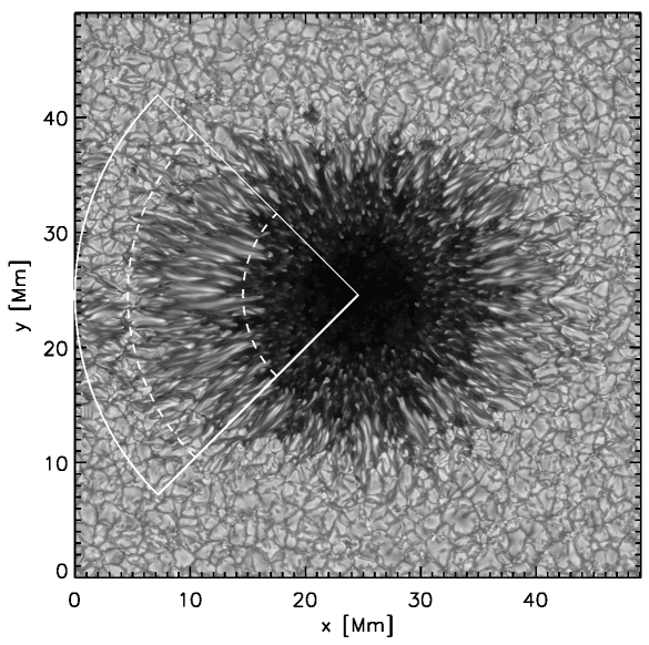
Figure 1.— Intensity image of the sunspot we analyze at about 6 hours after initialization of the simulation run. We show here only one half of the horizontal extent of the computational domain, which contains a pair of opposite polarity sunspots oriented in the x-direction. The panel is centered on the right sunspot in the simulation domain, which has a stronger magnetic field and is overall more coherent. Our analysis is focused on the penumbral region on the left side. The white lines indicate the region used for azimuthal averages.

Figure 2.— Azimuthal averages of quantities at the $\tau=1$ level as function of the distance from the spot center. The dotted vertical lines indicate the radial positions also shown in Fig. 1. Quantities shown are a) intensity relative to quiet sun, b) radial velocity (solid) and vertical rms velocity (dashed), c) vertical field strength (solid) and radial field strength (dashed), and d) field inclination with respect to vertical. Here, the solid line indicates the average inclination angle, while the dashed line indicates the inclination computed from the average field.

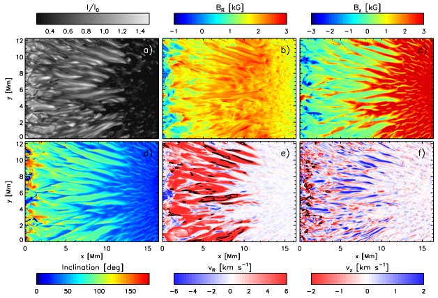
Figure 3.— Sunspot fine structure at the $\tau=1$ level. Quantities shown are a) bolometric intensity, b) radial and c) vertical magnetic field, d) field inclination, e) radial and f) vertical flow velocities. A field inclination of $0\deg$ corresponds to vertical field with the same polarity as the umbra, $90\deg$ to horizontal and $180\deg$ to vertical field with opposite polarity of the umbra. Radial outflows are displayed by red colors, solid contours indicate regions with more than $10\,\mbox{km\,s}^{-1}$ outflow velocity. Vertical upflows are displayed by blue colors, solid contours indicate regions with more than $5\,\mbox{km\,s}^{-1}$ downflow velocity.

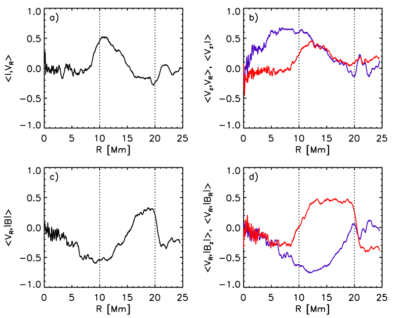
Figure 4.— a) Correlation between intensity and radial velocity ; b) correlation between vertical and radial velocity (blue) as well as vertical velocity and intensity (red); c) correlation between magnetic field strength and radial velocity; d) correlation between vertical field strength and radial velocity (blue) as well as radial field strength and radial velocity (red).

As described in detail in Rempel et al. (2009a), the simulation domain contains a pair of opposite polarity sunspots, with the most extended penumbrae found in between the opposite polarity spots along the horizontal x-direction. The most coherent penumbra is found in the sunspot with the initially stronger field strength of about $4$ kG (see the spot on the right in Fig. 1 of Rempel et al., 2009a). We focus our detailed analysis on the latter, for which an intensity image is presented in Fig. 1. We are here in particular interested in the extended penumbra on the left side of the spot for which we highlighted the sub-domain used for azimuthal averages in subsequent figures. The dashed lines indicate $R=10$ Mm and $R=20$ Mm from the center of the spot. Fig. 2 summarizes properties at the $\tau=1$ level, averaged azimuthally over the $90$ degree wedge shown in Fig. 1 and about $1$ hour in time. The intensity normalized by the quiet Sun brightness $I_{\odot}$ (panel a) shows a sharp increase from umbra toward penumbra from about 0.15 to 0.7 $I_{\odot}$. In the inner penumbra, the intensity stays constant on a plateau with about $0.7I_{\odot}$ and increases then almost linear toward the edge of the penumbra where it reaches $0.95I_{\odot}$ (due to the nearby opposite polarity spot in our simulation setup the intensity does not reach $I_{\odot}$). The plateau-like intensity profile formed during later stages of this simulation and was not present in the results reported earlier by Rempel et al. (2009a). The radial outflow (panel b) starts at about $R=10$ Mm, reaches its peak of about $4\,\mbox{km\,s}^{-1}$ near $R=15$ Mm and drops off toward the outer edge of the penumbra. $R=10$ Mm corresponds to the position at which the average field inclination (displayed in panel d) angle exceeds $45$ degrees, which was already found by Rempel et al. (2009a) as the critical value for the onset of large-scale outflows. The position of the peak velocity coincides with the position of maximum inclination (about 70 degrees) in the middle of the penumbra. The inclination is defined here as $\arcsin(B_{R}/|B|)$. Due to the strong variation of inclination angle with azimuth, it makes a difference whether we compute the inclination locally and average in azimuth and time later or whether we base the computation on the averaged magnetic field presented in panel c). We show in panel d) both, the average of the inclination (solid) and the inclination of the average field (dashed). The vertical rms velocity (panel b, dashed) increases steadily throughout the penumbra from a few $100\,\mbox{m\,s}^{-1}$ at $R=10$ Mm to about $2\,\mbox{km\,s}^{-1}$ at the outer edge, which is the value corresponding to quiet Sun granulation. A value of about $1\,\mbox{km\,s}^{-1}$ is required near the inner edge of the penumbra ($R=12$ Mm) to maintain the penumbral brightness of $0.7I_{\odot}$. We find in this simulation an approximate relationship of the form $I\propto\sqrt{v_{z\,rms}(\tau=1)}$.

3.2. Filamentation in photosphere

Fig. 3 displays the filamentary fine structure seen at the $\tau=1$ level in the penumbra. A filamentary structure is present in all quantities shown, however the strongest evidence is seen in intensity (panel a), vertical magnetic field (panel c), inclination (panel d) and radial flow velocity (panel e). Penumbral filaments show a strong reduction of the vertical magnetic field strength, while the horizontal (radial) field component is moderately enhanced (panel b). The combination of the two leads to the strong variation of the inclination angle in the penumbra. Strong radial outflows (panel e, red color indicates outflows) are seen in the almost horizontal flow channels, toward the outer end of flow channels the inclination angle exceeds $90\deg$, indicating field returning back into the convection zone. Radial outflows with more than $10\,\mbox{km\,s}^{-1}$ outflow velocity are indicated by solid contours. Most of the very fast outflows are found in the inner half of the penumbra, a few of them are associated with fast downflows in the outer penumbra. The vertical velocity (panel f, blue colors indicate upflows) shows strong up and downflows everywhere in the penumbra, strong radially aligned upflows are preferentially found in the center of penumbral filaments. Solid contours indicate regions with more than $5\,\mbox{km\,s}^{-1}$ downflow velocity. They are primarily found near the outer edge of the penumbra. We find downflow speeds of up to $15\,\mbox{km\,s}^{-1}$ near $\tau=1$. Fast downflows in opposite polarity regions have been observed by Westendorp Plaza et al. (2001); del Toro Iniesta et al. (2001).

To clarify the relation between radial flow velocity, intensity and magnetic field strength in a statistical sense we present correlation coefficients in Fig. 4. Panel a) displays the correlation between intensity and radial velocity, panel c) the correlation between field strength and radial velocity. All correlations are computed based on the fluctuations of these quantities about their azimuthal mean. Intensity is correlated with outflows in the inner penumbra, but weakly anti-correlated further outward. The radial outflow is found in regions with reduced field strength in the inner, but stronger field in the outer penumbra. Similar correlations were found by Ichimoto et al. (2007a) (see Fig. 3 therein) as well as Schlichenmaier et al. (2005). In the panels on the right (b and d) we present additional correlations, which allow us to make a closer connection to the magnetoconvective structure of the penumbra. The radial dependence of the $I-v_{R}$ correlation is due to a decorrelation between vertical and radial velocity in the penumbra (panel b, blue) combined with a decorrelation of vertical velocity and intensity (panel b, red). While the latter remains positive, a sign change is present in the former. The physical reason for the decorrelation between vertical and radial velocity is evident from the magnetoconvection pattern shown in Fig. 3. In the inner penumbra filaments are very narrow and the central upflow covers most of the filament, leading to large positive correlation between the brighter upflow and radial outflow. In the outer penumbra the patches of outflowing material become broader and several downflow lanes can be found within these patches, resulting in a reduction of the correlation. Toward the outer edge of the penumbra stronger downflow patches are present, turning the correlation weakly negative. Note that the $I-v_{z}$ correlation stays low outside $R=20$ Mm due to the proximity of an opposite polarity spot in our simulation setup. Fig. 4 panel d) presents additional correlations between radial velocity and vertical magnetic field (blue) as well as radial magnetic field strength (red). While the former stays negative throughout the penumbra, the correlation with the radial field strength is positive. In the innermost penumbra the strong reduction of $|B_{z}|$ dominates the picture and leads to an anti-correlation between $v_{R}$ and $|B|$, further out the contribution from the increased $|B_{R}|$ in the flow channels dominates and leads to a positive $v_{R}-|B|$ correlation. The increase of the inclination angle found in the flow channels is a consequence of a strong reduction of $B_{z}$ to almost zero, while $B_{R}$ is moderately enhanced in strength. This asymmetry is due to the fact that $B_{R}$ benefits from a strong positive contribution of the induction term $(\vec{B}\cdot\nabla)\vec{v}$ due to the Evershed flow, while the corresponding term is negative for $B_{z}$ due to the upward decreasing vertical velocity near $\tau=1$ (see Sect. 5 for more detail). Ichimoto et al. (2007a) found also a negative $v_{R}-|B|$ correlation in the inner penumbra with a trend of overall decreasing anti-correlation further out, however, a sign change was not observed. The latter was proposed by Tritschler et al. (2007) and Ichimoto et al. (2008) based on observations of the net circular polarization (NCP) in the outer penumbra at different viewing angles.

The outflow velocity we find in the simulation is not stationary, we see flow variability that ranges from periodic fluctuations on timescales of $5-10$ minutes in the inner penumbra to quasi-periodic variations over a wider range of timescales starting from $10-20$ minutes in the center and outer penumbra. A flow variability in the $15-40$ minute range was also reported in the simulation of Kitiashvili et al. (2009) and associated with Evershed clouds (Shine et al., 1994; Rimmele, 1994; Cabrera Solana et al., 2007). It is conceivable that the periodic variations we find near the inner tip of filaments have a relation to twisting motions observed by Ichimoto et al. (2007b) and Bharti et al. (2010). We focus in this paper on the maintenance of the stationary flow component and base our analysis primarily on time and volume averages over sections of the penumbra. The non stationary flow component will be analyzed in a separate publication.

3.3. Mass and energy fluxes

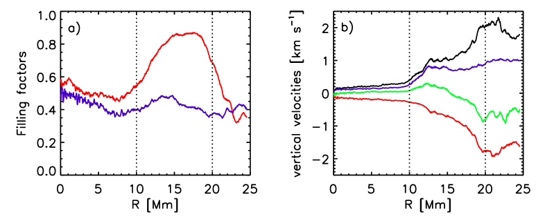
Figure 5.— a) Filling factors of radial outflows (red) and upflows (blue). b) Vertical rms velocity (black), mean upflow (blue), mean downflow velocity (red), and mean vertical velocity in regions with outflows (green).

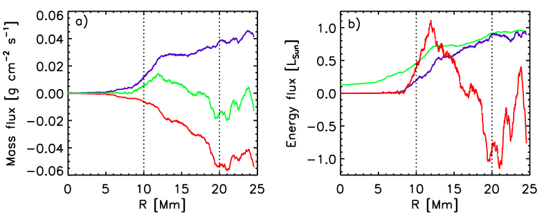
Figure 6.— a) Mass flux in upflows (blue), downflows (red), and azimuthal average of mass flux (green). In the inner penumbra up to $50\%$ of the total upward directed mass flux is found in the large-scale flow component. The vertical mass flux is balanced within $R<20.9$ Mm. In this region about $13\%$ of the unsigned mass flux is found in the large-scale flow component. b) Decomposition of convective energy flux into normalized small-scale energy flux (blue) and large-scale energy flux (red). In green color is shown the normalized surface intensity for comparison. Integrated over the region with balanced vertical mass flux ($R<20.9$ Mm), the contribution from the large-scale flow component is $12\%$, consistent with the mass flux contribution.

Fig. 5 panel a) displays filling factors of radial and vertical motions. While the upflow filling factor remains almost constant around $0.4$ to $0.5$ from inner umbra toward the outer penumbra, the filling factor of outflows exceeds $0.8$ in the center of the penumbra. Panel b) shows the vertical rms velocity (black), together with the mean velocity of upflow (blue) and downflow regions (red). The green line presents the mean vertical velocity averaged over regions with radial outflows (flow channels). The latter shows a weak average upflow of about $250\,\mbox{m\,s}^{-1}$ in the inner penumbra and a downflow reaching velocities of more than $500\,\mbox{m\,s}^{-1}$ toward the outer edge of the penumbra.

The contributions from small- and large-scale flow components to mass and energy flux in the penumbra are presented in Fig. 6. In order to properly compare up- and downflow components we perform the analysis here on a constant height surface that is located about $350$ km beneath $\tau=1$ in the quiet Sun (about half a Wilson depression downward). We decompose here the mass flux into positive and negative as well as azimuthal average components. Their contributions as function of radius are presented in panel a), where we show $\langle m_{z}^{+}\rangle$ in blue and $\langle m_{z}^{-}\rangle$ in red as well as $\langle m_{z}\rangle$ in green (the latter is the sum of the former two). Here, $\langle\ldots\rangle$ denotes the azimuthal average and $m_{z}^{\pm}=(m_{z}\pm|m_{z}|)/2$. While in the innermost penumbra up to about $50\%$ of the mass flux is present in the azimuthal average component, this fraction drops steadily toward the center penumbra. Integrated over the region $R<15$ Mm about $1/3$ of the total upward flowing mass is found in the azimuthal component, while the major fraction ($2/3$) is still overturning laterally. The mass flux in the penumbra is balanced within $R<20.9$ Mm. Integrated over this region the unsigned mass flux in the mean component constitutes about $13\%$ of the total unsigned vertical mass flux in the penumbra.

Evaluating the relative contributions from large-scale and small-scale convective motions to the total convective energy flux in the penumbra requires an appropriate decomposition of the vertical mass flux. A separation just into azimuthal mean and the respective fluctuation would not be sufficient since the latter assumes that the large-scale flow is axisymmetric and equally considers filaments with higher temperature and the region in between with lower temperature in the enthalpy flux. The consequence would be an underestimation of the overall contribution from the large-scale flow (in the region $R<20.9$ the net contribution would be $-0.07L_{\odot}$). Instead we construct the vertical mass flux of the laterally overturning flow component $m_{z}^{S}$ as follows: in regions with positive $\langle m_{z}\rangle$, we reduce the amplitude of upflows such that they are in a mass flux balance with downflows, in regions with negative $\langle m_{z}\rangle$, we reduce the amplitude of downflows such that they are in balance with the upward directed mass flux. The large-scale mass flux is then given by $m_{z}^{L}=m_{z}-m_{z}^{S}$. Unlike the decomposition into azimuthal mean and corresponding fluctuation, this procedure does not change the position of upflow and downflow regions for $m_{z}^{S}$ and $m_{z}^{L}$ compared to $m_{z}$. With $H=(e_{\rm int}+p)/\varrho+v^{2}/2$ we can now compute the energy flux components $F_{z}^{S/L}=\langle m_{z}^{S/L}H\rangle$, which are displayed in Fig. 6 panel b). While $F_{z}^{S}$ matches the intensity profile very well in the outer penumbra, there is a clear deficit present in the inner penumbra. The deviations in the umbra are due to the fact that our horizontal slice is located above the $\tau=1$ in the umbra and therefore the convective energy flux is zero. The large scale energy flux $F_{z}^{L}$ has an amplitude of about $+L_{\odot}$ in the inner penumbra and $-L_{\odot}$ in the outer penumbra. The relevant quantity here is the net contribution after carefully balancing the upflow in the inner and downflow in the outer penumbra. Integrating $F_{z}^{L}$ over the region $R<20.9$ Mm (in which the large-scale mass flux is balanced) leads to a net contribution of $12\%$ to the total convective energy flux. The latter is very consistent with the relative mass flux contribution of $13\%$ we found before. In an integral sense the large-scale flow contributes only a small fraction of the energy radiated away in a sunspot penumbra, but locally the contribution can be larger. If we use the difference between $F_{z}^{S}/L_{\odot}$ (blue) and $I/I_{\odot}$ (green) in Fig. 6 as a rough estimate for the missing energy flux we identify a contribution of up to $50\%$ in the inner penumbra. Note that we avoided in the above discussion the association between Evershed flow and the large-scale flow component since there is no clear definition of what the former encompasses. If we associate the Evershed flow only with the horizontal flow pattern that corresponds to upflows in the inner and downflows in the outer penumbra we would conclude that this flow pattern plays only a minor role in the penumbral energy transport. This definition would essentially correspond to the ”sources” and ”sinks” of the Evershed flow that have been identified by Rimmele & Marino (2006) and Ichimoto et al. (2007a). Also note that the contribution from large-scale flows increases with depth as all intrinsic scales of convection increase with depth. Properly quantifying their contribution in deeper layers requires numerical simulations over longer timescales (since convective timescales increase with depth), which is beyond the scope of the current investigation.

4. Subsurface flow structure and underlying driving forces

4.1. Flow structure beneath penumbra

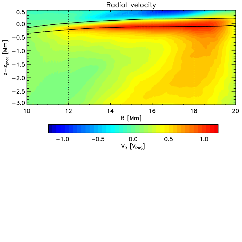
Figure 7.— Radial and depth dependence of radial flows in penumbra. The radial flow velocity is normalized with the rms velocity of convective motions outside the sunspot (which is shown in Fig. 8 panel a). The dark solid lines indicate the $\tau=1$ and $\tau=0.01$ levels. The strongest outflows reach velocities comparable to the rms velocity and are concentrated around $\tau=1$. We see a transition from outflow to inflow at about $\tau=0.01$ in the inner and at $\tau=0.001$ in the outer penumbra. In deeper layers, especially in the outer penumbra, outflows with speeds reaching $50\%$ of the convective rms velocity are present. The vertical dotted lines indicate sub-regions we use for a more detailed analysis in the following discussion.

Fig. 7 presents the subsurface outflow structure as function of depth and radial distance from the center of the spot. The depth is measured relative to the average height of the $\tau=1$ level in the quiet sun. We will use the same height scale in all of the following figures except Fig. 16, where we use the average $\tau=1$ level in the penumbra as reference. Flow velocities are normalized by the rms velocity found outside the sunspot at the corresponding height level (see also Fig. 8). We have chosen this normalization in order to compare flow fields found in the penumbra to convective flows found in almost undisturbed convection. We refer to this velocity reference in the following as $v_{\rm rms}^{0}$. While the outflow velocity stays around $0.4-0.5\,v_{\rm rms}^{0}$ in the deeper layers, the near surface layers stand out with flow speeds exceeding $v_{\rm rms}^{0}$. The two different scaling regimes of the outflow velocity found in the near surface layers (uppermost $500$ km) and the deeper part of the domain indicate already different physical driving mechanism at work, which we will analyze further in the following discussion. We exclude here the lower most $2$ Mm of our domain which are partially influenced by the bottom boundary condition. The solid black lines indicate the average $\tau=1$ and $\tau=0.01$ levels. The radial outflow velocity peaks close to $\tau=1$ and falls off rapidly with height. An outflow is present to about $\tau=0.01$ in the inner and $\tau=10^{-3}$ in the outer penumbra. The azimuthally averaged mass flux changes sign between $\tau=10^{-3}$ and $\tau=10^{-4}$, since it puts more weight on the region above the more dense filament channels with fast outflows. Overall the simulation indicates that radial outflows in the penumbra are expected to be found in the deep photosphere, which is consistent with recent spectropolarimetric inversions (Schlichenmaier et al., 2004; Bellot Rubio et al., 2006; Borrero et al., 2008), but not earlier work by Rimmele (1995) and Stanchfield et al. (1997) where elevated flow channels were inferred. Whether the inflow above $\tau=10^{-3}$ could be related to the inverse Evershed flow observed in the Chromosphere (Dialetis et al., 1985) is currently an open question, even though also Borrero et al. (2008) found observational evidence for an inflow near temperature minimum. As described in Rempel et al. (2009b) we switch for reasons of numerical stability to an isothermal equation of state in regions with $\beta=p_{\rm gas}/p_{\rm mag}<10^{-3}$ and limit the Lorentz force such that the Alfvén velocity does not exceed $60\,\mbox{km\,s}^{-1}$ to prevent stringent time step constraints. The latter two could possibly influence this flow pattern near the top boundary while the influence on flows in the photosphere is rather weak. Despite substantial velocities of a few $\mbox{km\,s}^{-1}$ the associated mass and momentum flux is negligible compared to photospheric flows due to the sharp drop in density.

The vertical dotted lines indicate 3 regions we refer to in the following analysis. We consider the region in between $R=10$ and $R=12$ Mm as inner penumbra, the region in between $R=12$ and $R=18$ Mm as center penumbra and $R=18$ and $R=20$ as outer penumbra. We have chosen the boundary for the inner penumbra based on the intensity profile (Fig. 2) that reaches a value typical for a penumbra of $0.7I_{\odot}$ at $R=12$ Mm. Since our outer penumbra might not be fully representative for conditions in a ”typical” outer penumbra due to the presence of a nearby opposite polarity spot with an Evershed flow in the opposite direction, we separated out regions with $R>18$ Mm. $R=18$ Mm is also the distance where most of the dominant filaments of the center penumbra end (see Fig. 1 and 3).

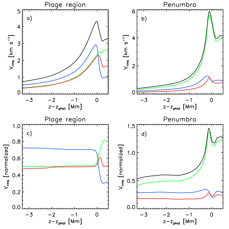
Figure 8.— Vertical profiles of rms velocities in the plage region surrounding the spot (a, c) and in the penumbra (b, d). The latter rms velocities are computed in the center penumbra in between $R=12$ and $R=18$ Mm. Panels a) and b) show the absolute values, while velocities in panels c) and d) are normalized by the rms velocity profile outside the sunspot near the edge of the computational domain. Black indicates the total, blue the vertical rms velocity, green and red the 2 horizontal components. In the case of the penumbra green is the component along the filaments. In the penumbra there are 2 distinct regimes. In the deep layers ($<-1$ Mm) flows are anisotropic, but show a depth dependence similar to convective flows in the plage region (i.e., they scale proportional to $v_{\rm rms}^{0}$). In the near surface layers, this scaling is still present for flows turning over laterally (blue and red curve), while the flow component along filaments shows a much steeper increase with height.

Fig. 8 compares rms velocities in the plage region surrounding the sunspot and the center penumbra. The top panels present the absolute rms velocities, the bottom panels relative to $v_{\rm rms}^{0}$. Blue indicates the vertical rms velocity, green and red the horizontal components (green is along the filaments in the case of the penumbra). In the plage region (more or less undisturbed convection) about half of the kinetic energy is found in vertical motions, the other half equally distributed among the horizontal components. This scaling holds very well over the 3 orders of magnitude in pressure stratification shown here (panel c). In the penumbra the vertical and horizontal rms velocity perpendicular to the filaments show a similar scaling and relative strength, but overall their amplitude is reduced to about $40\%$ of the respective values in the plage region. The rms velocity along the filaments is strongly increased with respect to the vertical rms, indicating a strong degree of anisotropy. The rms velocity in the direction of filaments is proportional to $v_{\rm rms}^{0}$ in more than $1$ Mm depth and shows a steep increase toward the photosphere. Overall the kinetic energy is reduced in the deeper layers, but doubled in the near surface layers compared to the plage region. The apparent excess of kinetic energy found in the Evershed flow compared to the plage region is due to a vertical redistribution of kinetic energy combined with anisotropy of the flow.

4.2. Underlying driving forces

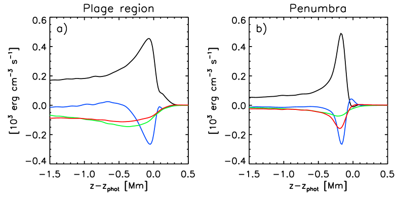
Figure 9.— Comparison of energy conversion terms in kinetic energy equation between plage region (a) and center penumbra (b). The quantities shown are averaged in volume and about 1 hour in time. Black: work by pressure/buoyancy forces; red: work by Lorentz force; blue: work by acceleration forces; green: work by viscous forces. Overall the pressure/buoyancy forces are the primary driver of flows. Close to the surface a major fraction of the energy is deposited into acceleration work, viscous losses and work against Lorentz forces have about equal contributions.

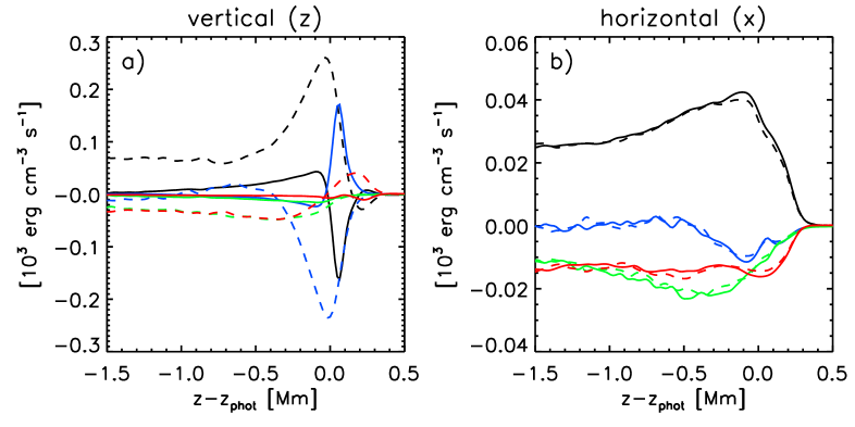
Figure 10.— Plage region: Energy conversion terms in kinetic energy equation. The quantities shown are averaged in volume and about 1 hour in time. Black: work by pressure/buoyancy forces; red: work by Lorentz force; blue: work by acceleration forces; green: work by viscous forces. Solid lines indicate upflow, dashed lines downflow regions. a) Contribution from terms in the vertical and b) from terms in the horizontal direction. In the vertical momentum equation pressure/buoyancy terms are in balance with acceleration terms. Most pressure/buoyancy driving takes place in the downflow regions. In the horizontal momentum equations pressure driving is offset primarily by work against magnetic and viscous forces.

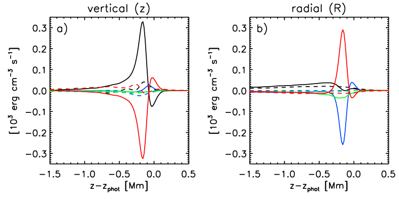
Figure 11.— Center penumbra (averaged in between $R=12$ to $R=18$ Mm): Quantities shown are the same as in Fig. 10. In the vertical momentum equation (panel a) pressure driving is balanced by by work against the Lorentz force. Contrary to the plage region the pressure driving takes place in upflow regions. Acceleration terms are negligible. In the radial direction (panel b) outflows are primarily driven by magnetic forces (in the uppermost few $100$ km), which are in balance with acceleration terms. In deeper layers pressure driving becomes more important, but remains weaker than in the plage region (see also Fig. 12).

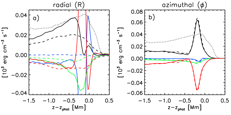
Figure 12.— Energy conversion terms for the radial direction in the center penumbra on different scale (panel a). In more than $300$ km depth flows are primarily driven by pressure forces. Pressure driving favors outflows, the Lorentz force opposes inflows more than outflows. In less than $300$ km depth, the Lorentz force is the dominant driver for outflows, while pressure driving favors inflows. Panel b) shows the balance for horizontal motions perpendicular to the filaments (azimuthal direction). Work by pressure forces is in balance with work against magnetic forces. The dotted line indicates in both panels the role of pressure driving in the plage region for comparison.

In order to investigate the physical processes that lead to the driving of large-scale outflows around sunspots we analyze the energy conversion terms in the kinetic energy equation. Starting from the momentum equation we derive the following energy balance (we drop the time derivatives since we are interested in time averages):

$$\begin{split}\underbrace{\vec{v}\cdot(\varrho\vec{g}-\nabla p)}_{\rm pressure/buoyancy}&+\underbrace{\vec{v}\cdot(\vec{j}\times\vec{B})}_{\rm Lorentz}\\ &\underbrace{-\varrho\vec{v}\cdot[(\vec{v}\cdot\nabla)\vec{v}]}_{\rm Acceleration}+\underbrace{\vec{v}\cdot F_{visc}}_{\rm Viscosity}=0\;.\end{split}$$ (1)

Under the assumption of stationarity the acceleration term is identical to the negative divergence of the kinetic energy flux, $\varrho\vec{v}v^{2}/2$. A negative acceleration term implies positive divergence, i.e. the volume element is a source of kinetic energy. In Fig. 9 we compare the different contributions to the energy equation for the plage region (panel a) and penumbra (panel b). On a qualitative level there is a large degree of similarity: Pressure/buoyancy forces are the main driver, close to the surface most of that energy input is used up by acceleration forces, the remainder is balanced in about equal parts by work against viscous and Lorentz forces. In the penumbra the total amount of energy input by pressure/buoyancy forces in the uppermost $1.5$ Mm shown here is reduced to about $40\%$ and more concentrated toward the photosphere. The reduction in energy input is consistent with the overall reduced kinetic energy integrated over this depth range. It is also notable that the work against the Lorentz force is not substantially different from the plage region (relative to the respective pressure driving) despite the quite different field strength and field structure.

To investigate the driving of flows in plage and penumbra further we split now terms into the contributions from different grid directions as well as flow directions, i.e. we consider the following $18$ terms:

$$P_{i}^{\pm} = \langle\,v_{i}^{\pm}[\varrho g_{i}-(\nabla p)_{i}]\,\rangle$$ (2)

$$L_{i}^{\pm} = \langle\,v_{i}^{\pm}(\vec{j}\times\vec{B})_{i}\,\rangle$$ (3)

$$A_{i}^{\pm} = -\langle\,\varrho v_{i}^{\pm}[(\vec{v}\cdot\nabla)\vec{v}]_{i}\,\rangle$$ (4)

Here, $i$ indicates either the Cartesian directions $x,y,z$ in the case of the plage region or the cylindrical components $R,\Phi,z$ in the case of the sunspot penumbra. With $v_{i}^{\pm}=(v_{i}\pm|v_{i}|)/2$ we denote negative and positive velocity components. Note that we compute all forces on the Cartesian grid and use the transformation to cylindrical coordinates only to separate the directions along and perpendicular to filaments in our nearly axisymmetric penumbra fragment (i.e. we compute terms like $v_{r}F_{r}$ and $v_{\Phi}F_{\Phi}$ instead of $v_{x}F_{x}$ and $v_{y}F_{y}$ with $\vec{F}$ being any one of the forces). The explicit expression for the viscous force is rather complicated due to the non-linearity of the underlying artificial viscosity scheme. In the following discussion we do not explicitly compute the viscous terms, but indicate their approximate magnitude by using the quantity $V_{i}^{\pm}=-(P_{i}^{\pm}+L_{i}^{\pm}+A_{i}^{\pm})$. We confirmed a close relationship for a few snapshots, for which we restarted the code and extracted all numerical dissipation terms.

Formally the energy conversion terms are power densities (work per volume and time). For the sake of making the text more readable we will refer to them in the following discussion very often as ”work done by/against … forces” instead of ”work done by/against … forces per volume and time”. Since the former is simply the latter multiplied by a unit volume element and time interval it has no further impact on the physical meaning of these terms.

Fig. 10 shows the energy conversion terms for vertical motions (panel a) and horizontal motions (panel b) in the plage region. Note that we only show one horizontal direction due to isotropy. In the vertical direction pressure/buoyancy driving is in balance with work done against acceleration forces. Most of the pressure/buoyancy driving takes place in downflows due to their overdense material that cannot be supported by the pressure gradient. Pressure/buoyancy driving in upflows is much weaker since they are very close to a hydrostatic balance. Close to $z=0$ the sign of pressure/buoyancy driving is changing in upflows as a consequence of the overshoot layer in the upper photosphere. Magnetic and viscous forces play only a minor role in the vertical direction. Horizontal flows are primarily driven by pressure forces. Most of the energy is absorbed by magnetic and viscous forces, only a small amount is balanced by horizontal acceleration in the uppermost $500$ km of the convection zone.

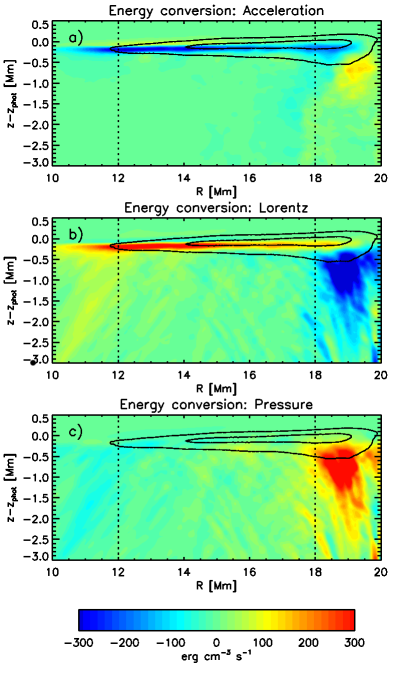
Figure 13.— Energy conversion terms as functions of radius and depth in the penumbra. We show the differences between the energy conversion for outflow and inflow regions. Panel a) shows $A^{+}_{R}-A^{-}_{R}$, panel b) $L^{+}_{R}-L^{-}_{R}$, and panel c) $P^{+}_{R}-P^{-}_{R}$. The contour lines indicate regions with average outflows of more than $2$ and $4\,\mbox{km\,s}^{-1}$.

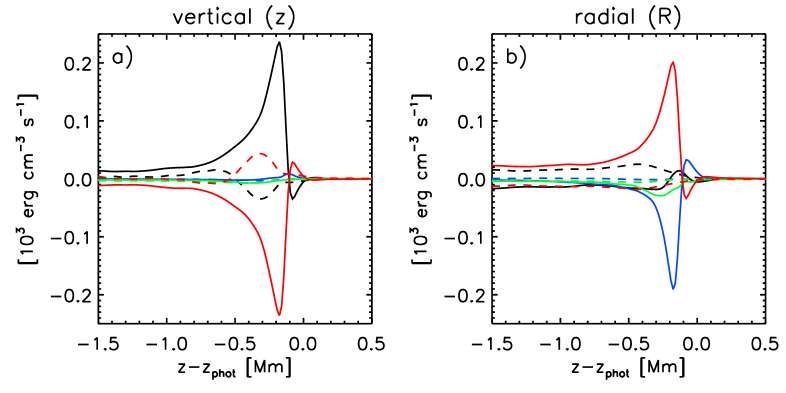
Figure 14.— Inner penumbra (averaged in between $R=10$ to $R=12$ Mm): Quantities shown are the same as in Fig. 10.

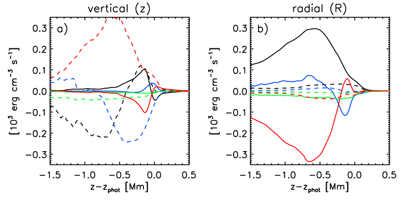
Figure 15.— Outer penumbra (averaged in between $R=18$ to $R=20$ Mm): Quantities shown are the same as in Fig. 10.

In comparison to the plage region, the center penumbra shows distinct differences (Fig. 11). Almost all pressure/buoyancy driving takes place in upflow regions: the presence of strong magnetic field causes in the near surface layers to a steepening of the pressure gradient, leading to almost hydrostatic balance in downflows and excess pressure driving in the upflows. This excess pressure driving in upflows is in balance with work against the Lorentz force while in contrast to the plage region vertical acceleration of fluid does not play an important role at all. Most of the energy extracted by Lorentz forces in the vertical direction is deposited into outward acceleration of fluid along filaments. In that sense the Evershed flow is driven by vertical pressure forces in upflows that are deflected into the horizontal direction through the Lorentz-force. This ”deflection” is most efficient very close to the surface: integrated from $1$ Mm ($500$, $250$ km) depth to the top boundary about $44\%$ ($64\%$, $97\%$) of the pressure driving in the vertical direction ends up as Lorentz force driving in the radial direction. This way kinetic energy that is normally deposited into the vertical direction (plage region) gets transferred directly into the horizontal direction and accounts for the high anisotropy seen in the penumbra.

Also the role of horizontal pressure driving differs substantially from the plage region, which can be seen in Fig. 12a), where we show the energy conversion terms for the radial direction on a different scale. Pressure driving is dominant below $300$ km depth, but the overall magnitude remains smaller than in the plage region at comparable depth. While pressure driving shows a preference for outflows in more than $300$ km depth, it prefers inflows further up. Pressure forces are the primary cause for the deep flow component with velocities of about $0.5\,v_{\rm rms}^{0}$ we identified in Fig. 7, but their overall role for the near surface flow is limited: integrated from $1$ Mm ($500$, $250$ km) depth to the top boundary the contribution from $P^{+}_{R}$ relative to $L^{+}_{R}$ is $100\%$ ($38\%$, $9\%$). If we consider only the components of the driving that break the symmetry between in- and outflows, $P^{+}_{R}-P^{-}_{R}$ and $L^{+}_{R}-L^{-}_{R}$, the corresponding values are $13\%$ ($1\%$, $-9\%$). Note that most of the contribution to $P^{+}_{R}-P^{-}_{R}$ comes from the region $R>17$ Mm, further inward $P^{+}_{R}-P^{-}_{R}$ is close to zero (see also Fig. 13).

However, pressure forces remain the dominant driver for flows perpendicular ($\Phi$-direction) to filaments (Fig. 12b). Here, pressure driving is offset by work against the Lorentz force, while both acceleration and viscous terms do not contribute substantially.

The different role of pressure driving compared to the plage region is primarily a consequence of anisotropy in terms of radially elongated convection cells in the penumbra: radial pressure gradients are reduced, while lateral pressure gradients are enhanced compared to isotropic granulation. In addition the steepening of the vertical pressure gradient (that leads to the shift of pressure driving from down to upflows) results in an overall reduction of pressure close to the photosphere in comparison to the ambient stratification.

The clear association between Lorentz force driving and the near surface flow pattern is evident from Fig. 13. Here, we present the quantities $A^{+}_{R}-A^{-}_{R}$, $L^{+}_{R}-L^{-}_{R}$ and $P^{+}_{R}-P^{-}_{R}$ as function of radius and depth. Strong negative values of $A^{+}_{R}-A^{-}_{R}$ indicate outward acceleration of fluid. These regions are confined to a narrow layer near $\tau=1$. Here, the Lorentz force is the primary driver, pressure terms have weakly negative contributions (they favor inflows). The peak of Lorentz force driving and acceleration is found in between $R=12$ and $R=15$ Mm.

In deeper layers pressure terms are in approximate balance with Lorentz force terms, resulting in only minor acceleration work despite their overall amplitude. Toward the outermost edge the Lorentz force is overcompensating outward directed pressure driving resulting in deceleration of radial outflows (positive values of $A^{+}_{R}-A^{-}_{R}$).

For comparison with Fig. 11 we present in Figs. 14 and 15 the same quantities for the inner penumbra (from $R=10$ to $R=12$ Mm) and outer penumbra (from $R=18$ to $R=20$ Mm).

In the inner penumbra we see a forcing pattern that is very similar to that we found for the center penumbra, in particular with respect to the near surface layers where the Evershed flow is driven. Differences are present in deeper layers; here, the Lorentz force is also dominant in driving outflows and is actually driving these outflows against horizontal pressure forces.

In the outer penumbra, we see a fundamentally different situation (which is in part a consequence of the nearby opposite polarity spot and the resulting strongly magnetized downflow lane in between). Here, outward directed pressure forces dominate the picture entirely, however, they do not lead to a strong outward acceleration of fluid. To a large degree they are opposed by the horizontal Lorentz force and the energy is transferred to the vertical direction, where the Lorentz force becomes the major driver for downflows. The latter is due to the fact that magnetic field in the outer penumbra turns back downward. We see in the uppermost layers only a weak signal from the horizontal Lorentz force driving outflows – this is expected since we are in the region where the Evershed flow declines quickly to zero.

We will further discuss the deeper reaching flow component in Sect. 21.

5. Magnetic filament substructure responsible for driving the Evershed flow

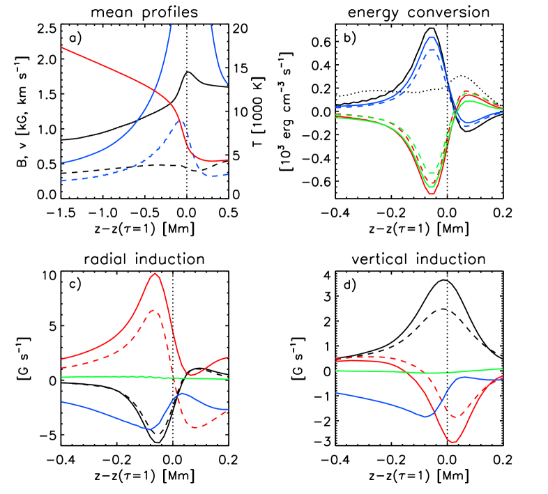
Figure 16.— a) Average vertical thermal, magnetic and flow profiles in regions responsible for driving the Evershed flow. Magnetic field (black) and flow profiles (blue) are shown on the left scale, solid lines indicate the radial, dashed lines the vertical component. The temperature (red) is shown on the right scale. b) Pressure driving in upflows (black), work against Lorentz force in upflows (red), work by Lorentz force in radial direction (blue) and work against acceleration forces in radial direction (green). The dashed lines show simplified expressions that are explained in the text. The dotted line indicates the contribution from horizontal pressure gradients multiplied by a factor of $10$. Bottom panels: Contributions in induction equation from advection (black), field line stretching (red), flow divergence (blue) and numerical diffusivity (green). Panel c) displays terms for the radial and panel d) for the vertical field component. Here, dashed and dotted lines refer again to simplified expressions explained in the text. Vertical dotted lines indicate the average $\tau=1$ level.

5.1. Simplified momentum balance

After describing the driving forces behind the Evershed flow in detail in the previous section, we present here a simple model of the underlying thermal, magnetic and velocity structure and reduce the overall picture to the most relevant terms in the equations. In order to carve out the typical structure of the regions responsible for driving the Evershed flow we select regions which have both upflows and outflows. In Fig. 16a) we present the mean magnetic field, flow, and thermal structure as function of depth obtained by averaging over all such regions horizontally between $R=12$ and $R=18$ Mm. While the vertical magnetic field (black, dashed) is constant at about $400$ G, the radial component (black, solid) increases monotonically from about $900$ G to $1.8$ kG at the $\tau=1$ level (vertical dotted line) and drops again in higher layers to about $1.6$ kG. The steep increase just below $\tau=1$ is essential for the Lorentz force component driving the outflow as we will describe below. The vertical velocity (blue, dashed) increases monotonically to about $1\,\mbox{km\,s}^{-1}$ just $100$ km beneath $\tau=1$, followed by a sharp decline to a few $100\,\mbox{m\,s}^{-1}$ above $\tau=1$. The radial flow velocity peaks right at $\tau=1$, the maximum amplitude is about $5.5\,\mbox{km\,s}^{-1}$. The solid red line shows the mean temperature profile with the corresponding scale on the right. Panel b) presents volume averages of pressure driving in upflows (black) work against Lorentz force in upflows (red) and work by Lorentz force in outflows (blue) and work against acceleration forces (green) for the same region. The dotted black line shows contributions from horizontal pressure gradients multiplied by a factor of $10$. Averaged over the region shown (from -$0.4$ to $0.2$ Mm) they contribute about $10\%$ to the total acceleration work. Work by the horizontal Lorentz force (blue) is $90\%$ of the work by vertical pressure driving (black). The solid lines are based on all terms in the equations (see Eqs. (2) to (4) ), the dashed lines are an approximation for Lorentz force and acceleration terms based only on volume averages of the following expressions:

$$L_{z} = -v_{z}\frac{1}{4\pi}B_{R}\frac{\partial B_{R}}{\partial z}$$ (5)

$$L_{R} = v_{R}\frac{1}{4\pi}B_{z}\frac{\partial B_{R}}{\partial z}$$ (6)

$$A_{R} = -\varrho v_{R}v_{z}\frac{\partial v_{R}}{\partial z}\;.$$ (7)

The excellent agreement allows us to understand the driving mechanism behind the Evershed effect by considering a reduced set of equations. Note that we could go even one step further with these simplifications, by expressing all terms through the mean quantities $\bar{B}_{R}(z)$, $\bar{B}_{z}(z)$, $\bar{v}_{R}(z)$, $\bar{v}_{z}(z)$, $\bar{p}(z)$, and $\bar{\varrho}(z)$. Despite the fact that we are dealing with nonlinear terms of spatially highly inhomogeneous quantities, the agreement remains excellent except for the acceleration term that falls short by a factor of 2, i.e. quantities such as $\overline{\varrho v_{R}v_{z}\partial_{z}v_{R}}$ and $\bar{\varrho}\bar{v}_{R}\bar{v}_{z}\partial_{z}\bar{v}_{R}$ agree in general on a qualitative level for the region we selected to perform the averages.

In the vertical direction we have essentially a magneto-hydrostatic balance involving the terms:

$$\overline{\frac{\partial}{\partial z}\left(p+\frac{B_{R}^{2}}{8\pi}\right)}\approx-\overline{\varrho g}\;.$$ (8)

This is evident from the opposing contributions of the terms $-\overline{v_{z}\left(\partial_{z}p+\varrho g\right)}$ and $-\overline{v_{z}B_{R}\partial_{z}B_{R}/(4\pi)}$ in Fig. 16b) (black and dashed red curve). The energy extracted by the Lorentz force in the vertical direction leads to a strong acceleration of an outflow in the radial direction. Here, we have a balance between the Lorentz force and acceleration terms:

$$\overline{\frac{1}{4\pi}B_{z}\frac{\partial B_{R}}{\partial z}}\approx\overline{\varrho v_{z}\frac{\partial v_{R}}{\partial z}}\;.$$ (9)

The acceleration force results from the upward transport of plasma in a region with an upward increasing Evershed flow velocity. The work by vertical and radial Lorentz force components is in approximate balance, i.e.

$$\overline{v_{z}\frac{1}{4\pi}B_{R}\frac{\partial B_{R}}{\partial z}}\approx\overline{v_{R}\frac{1}{4\pi}B_{z}\frac{\partial B_{R}}{\partial z}}\;,$$ (10)

leading to a simple relation between vertical and radial flow velocities of the form

$$\overline{v_{z}B_{R}}\approx\overline{v_{R}B_{z}}\;.$$ (11)

The latter is the relation one would expect from a simple ”deflection” of vertical flows by an inclined magnetic field.

Note that most of the acceleration of the outflow takes place about $100$ km beneath the $\tau=1$ level, while the outflow peaks right at $\tau=1$. The latter is a consequence of the strong vertical upflow advecting accelerated fluid a few $100$ km further upward. This upward advected fluid also overpowers the inward directed Lorentz force found right above $\tau=1$ due to the sign change in $\partial_{z}B_{R}$.

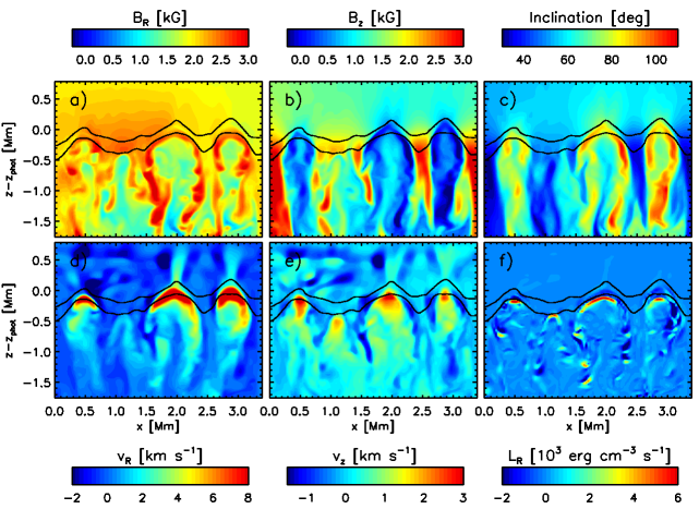
Figure 17.— Vertical cross section of filaments in the inner penumbra. Displayed are a) radial and b) vertical field strength together with the resulting inclination in panel c). The bottom panels show d) radial, e) vertical velocity and f) the energy conversion by the horizontal Lorentz force along filaments. The two solid lines indicate the $\tau=1$ and $0.01$ levels. The enhancement of $B_{R}$ combined with a reduction of $B_{z}$ around $\tau=1$ leads to a sharp increase of the inclination angle. The strong increase of the inclination angle is restricted to a very narrow boundary layer near $\tau=1$, around which we also see the dominant contribution from the horizontal Lorentz force. The resulting outflow found around $\tau=1$ is broader than the boundary layer, but also restricted to the deep photosphere.

5.2. Induction equation

Since the large positive value of $\partial_{z}B_{R}$ right below $\tau=1$ plays an essential role in the acceleration process, we analyze now how this magnetic field structure is maintained in the presence of strong vertical and radial flows. To this end we evaluate the different contributions in the induction equation:

$$\frac{\partial\vec{B}}{\partial t}=\underbrace{-(\vec{v}\cdot\nabla)\vec{B}}_{\rm Advection}+\underbrace{(\vec{B}\cdot\nabla)\vec{v}}_{\rm Stretching}\underbrace{-\vec{B}(\nabla\cdot\vec{v})}_{\rm Divergence}\;.$$ (12)

The bottom panels of Fig. 16 present these contributions (black: advection, red: stretching, blue: divergence) for the maintenance of the radial magnetic field structure in panel c) and vertical magnetic field structure in panel d). As before solid lines show the full expressions, dashed-line approximations are described in the text below. For the radial field component (panel c) the dominant source is the stretching term in the induction equation. The major contribution to this term comes from the vertical shear profile of the Evershed flow, leading to an induction term $\overline{B_{z}\partial_{z}v_{R}}$ (red dashed line). The remainder is due to horizontal stretching from terms like $\overline{B_{R}\partial_{R}v_{R}}$. The peak of the stretching term (including all contributions) is located about $100$ km beneath $\tau=1$, where we also find the peak of the Lorentz force driving. This is not exactly where we find the peak of $\bar{B}_{R}$, since there is an additional strong contribution from the vertical advection that pushes strong radial field upward ($-\overline{v_{z}\partial_{z}B_{R}}$, black dashed line). The remainder is offset by the negative contribution from the diverging convective motions (solid blue line). In the case of the vertical field (panel d), the role of the contributions from advection and stretching are opposite. Here ,advection is the primary mechanism that maintains the field. The positive sign originates primarily from horizontal advection terms (black dashed) with a dominant contribution from $-\overline{v_{R}\partial_{R}B_{z}}$ due to the on average outward decreasing vertical field strength, but there are also positive contributions from vertical advection $-\overline{v_{z}\partial_{z}B_{z}}$. The dominant negative contribution to the stretching term is due to $\overline{B_{z}\partial_{z}v_{z}}$ (red dashed line), which peaks close to $\tau=1$ where $\partial_{z}\bar{v}_{z}$ is strongly negative. The remainder is offset again by the negative contribution from the diverging convective motions (solid blue line). In both panels the green curve indicates the negative sum of these three terms, i.e. the amplitude of additional contributions from artificial numerical diffusivity. For both radial and vertical magnetic field the contributions from stretching, advection and divergence are in balance at the level of a few $\%$. This indicates that the magnetic structure within the penumbral filaments in this simulations is not strongly affected on average by the unavoidable artificial magnetic diffusivity of the numerical scheme. Also the fact that our simulation contains almost field free umbral dots on scales even smaller than filaments sets strong constraints on the role artificial diffusivity plays.

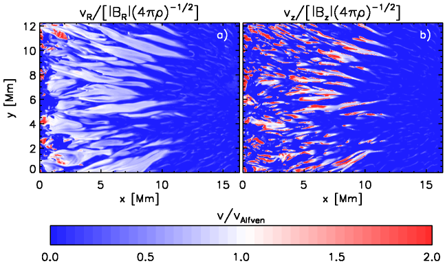
Figure 18.— Displayed are a) outflow and b) upflow velocities at $\tau=1$ relative to $|B_{R}|/\sqrt{4\pi\varrho}$ and $|B_{z}|/\sqrt{4\pi\varrho}$, respectively. Blue (white, red) colors indicate sub-Alfvénic (Alfvénic, super-Alfvénic) flow speeds. Throughout most of the penumbra the outflows stay close to $0.8\,|B_{R}|/\sqrt{4\pi\varrho}$.

5.3. Filament cross section

From Fig. 16 we deduce a vertical extent of about $200$ km for the region in which most of the energy conversion takes place. This value is obtained through an average over all areas between $R=12$ and $R=18$ km that have upflows and outflows. Since the typical height variation of the $\tau=1$ level in the penumbra is about $200$ km, this indicates that locally within individual filaments the flow is driven in an even narrower boundary layer right beneath the $\tau=1$ level. We illustrate this in Fig. 17, which shows magnetic field and velocity together with inclination and energy conversion by horizontal Lorentz force on a vertical cut through three developed and one just forming penumbral filament in the inner penumbra. It is evident that there is a narrow boundary layer forming along the $\tau=1$ surface that is characterized by increased $B_{R}$ and reduced $B_{z}$, resulting in a strong increase of inclination. Lorentz force driving is concentrated to an equally thin layer just beneath $\tau=1$, the resulting outflow is broader and extends above $\tau=1$. The latter is a consequence of the presence of overturning motions that transport and distribute accelerated fluid above and along the $\tau=1$ surface. This redistribution does not require additional acceleration work, since the associated kinetic energy flux is close to divergence free (the term for acceleration work is identical to the negative divergence of the kinetic energy flux under the assumption of stationarity). In Fig. 17, we highlighted a cross section in the inner penumbra, further out the filamentary structure is less prominent. Nevertheless, we also see there a concentration of the energy conversion terms to very thin sheets beneath $\tau=1$, while fast outflows are found mostly between $\tau=1$ and $\tau=0.01$. In a statistical (average) sense the differences between inner and center penumbra are small (compare Figs. 11 and 14). Also note that the concentration of energy conversion by Lorentz forces to thin sheets is typical for magnetoconvection in a more general sense; however, the preferred location and quasi-steady maintenance of these regions near $\tau=1$ is restricted to the penumbra. The mechanism responsible for the latter is explained in Sect. 5.4.

5.4. Formation of thin boundary layer

In this section we illustrate the crucial role of the vertical advection terms by discussing a simplified model that captures the essential terms on a qualitative level to within a factor of two. We consider only those terms in the radial momentum and induction equations that have been identified as the dominant contributors in the previous discussion:

$$\frac{\partial v_{R}}{\partial t}+v_{z}\frac{\partial v_{R}}{\partial z} = \frac{B_{z}}{4\pi\varrho}\frac{\partial B_{R}}{\partial z}$$ (13)

$$\frac{\partial B_{R}}{\partial t}+v_{z}\frac{\partial B_{R}}{\partial z} = B_{z}\frac{\partial v_{R}}{\partial z}\;.$$ (14)

Neglecting the advection terms, Eqs. (13) and (14) lead to wave solutions of the form (assuming that $B_{z}$ is nearly constant, which is at least true for the average shown in Fig. 16):

$$\left[\frac{\partial^{2}}{\partial t^{2}}-\frac{B_{z}^{2}}{4\pi\varrho}\frac{\partial^{2}}{\partial z^{2}}\right](v_{R},B_{R})=0\;.$$ (15)

In this case the profiles of $v_{R}$ and $B_{R}$ could not be maintained in place and would spread out with the Alfvén velocity corresponding to the vertical magnetic field component, $|B_{z}|/\sqrt{4\pi\varrho}$; see, for example, Vasil & Brummell (2009) for a discussion of the dynamics of magnetic shear layers. Since the Alfvén velocity is of the order of $2\,\mbox{km\,s}^{-1}$ (using a mean value of $B_{z}=400$ G and $\varrho=3\cdot 10^{-7}{\rm g}/{\rm cm}^{3}$ near the $\tau=1$ level), the rather narrow Evershed flow profile would broaden substantially within a few $100$ secs of time. On the other hand, the inclusion of the advection terms allows for a stationary solution provided that $v_{z}>|B_{z}|/\sqrt{4\pi\varrho}$. Since near $\tau=1$ the vertical field strength drops and upflows can reach locally up to $3\,\mbox{km\,s}^{-1}$, this condition can be met within the thin boundary layer in which most of the driving is taking place. With a sufficiently strong advection term the upflow counteracts the downward traveling Alfvén wave, while the upward traveling wave is bound by the photosphere and transition to a low $\beta$ regime. The quasi-steady maintenance of the shear layer despite the back-reaction of Lorentz forces seems to be at odds with Lenz’s rule, however, we have to keep in mind that there is a steady flow of energy through the system ultimately driven by overturning convective motions. Indeed, the energy conversion by the vertical advection term in the induction equation, $B_{R}/(4\pi)\,v_{z}\partial_{z}B_{R}$, is identical to the energy extracted by the Lorentz force from convective motions in the vertical direction (Eq. 5).

To summarize, the most important feature responsible for driving the Evershed flow is a strong increase of $B_{R}$ just beneath the $\tau=1$ level (combined with the presence of a vertical background field of a few $100$ G). The steep gradient of $B_{R}$ is primarily maintained by the vertical shear profile of the Evershed flow in combination with upward advection due to the strong upflow in the center of the filament. The vertical advection terms in the induction as well as momentum equation are essential for a quasi-stationary configuration with lifetimes far beyond the overturning timescale of convection. They ensure that the peak of $v_{R}$ and $B_{R}$ is maintained above the region with the strongest Lorentz force driving as well as induction due to shear, which are proportional to $\partial_{z}B_{R}$ and $\partial_{z}v_{R}$, respectively. The vertical confinement of the shear layer is guaranteed by the fact that locally the upflow velocity can exceed $|B_{z}|/\sqrt{4\pi\varrho}$. Since the outflow velocity is linked to the upflow velocity by the approximate relation $v_{R}B_{z}\approx v_{z}B_{R}$ the expectation is that the resulting outflow reaches a velocity of about $v_{R}=|B_{R}|/\sqrt{4\pi\varrho}$. With $B_{R}=1\ldots 2$ kG and $\varrho=3\cdot 10^{-7}{\rm g}{\rm cm}^{-3}$ the resulting velocities should be $v_{R}=5\ldots 10\,\mbox{km\,s}^{-1}$, which is about the range we find for the velocity within flow channels. Fig. 18 displays outflow and upflow velocities at $\tau=1$ relative to $|B_{R}|/\sqrt{4\pi\varrho}$ and $|B_{z}|/\sqrt{4\pi\varrho}$. Outflows are close to Alfvénic throughout the penumbra (typically $v_{R}\approx 0.8\,|B_{R}|/\sqrt{4\pi\varrho}$), upflows are weakly super-Alfvénic.

The fact that there is a clear threshold for the onset of this driving mechanism ($v_{z}>|B_{z}|/\sqrt{4\pi\varrho}$ near $\tau=1$) is a possible explanation for a more or less well defined inner edge of the penumbra, or related, a critical field inclination that needs to be exceeded (about $45$ degrees in this simulation). Going further inward toward the umbra the vertical field becomes stronger while vertical velocities are reduced, which makes it harder to pass this threshold locally. Even if it would be passed the resulting radial flow velocities would be less due to the smaller value of $B_{R}$.

5.5. Observable consequences

Unfortunately the ”feature” responsible for driving the Evershed flow remains well hidden beneath the $\tau=1$ level. Even worse, if we compute the Lorentz force from the ”visible” part of the magnetic field structure, the Lorentz force is inward directed due to the sign change of $\partial_{z}B_{R}$. The amplitude of the visible inward component above $\tau=1$ is about a factor of $5-10$ smaller than the strong outward directed component beneath $\tau=1$, which is responsible for the outward acceleration.

The observable parts of the magnetic and velocity field are an increase of $v_{R}$ and $B_{R}$ toward $\tau=1$ and a strong vertical gradient of $v_{z}$ around $\tau=1$. The latter is only visible very deep in the photosphere. The combination of this three factors should lead to positive values of ${\rm d}|B|/{\rm d}\tau$ and ${\rm d}|v_{\rm los}|/{\rm d}\tau$ for a variety of observation angles and therefore contribute to the net circular polarization observed in sunspot penumbrae.

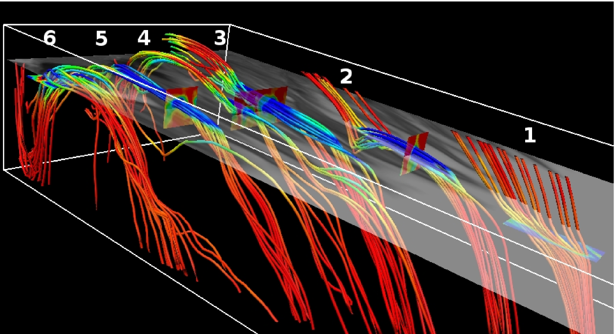
Figure 19.— Field line connectivity and associated horizontal flow speeds in simulated penumbra. The color of the field lines indicates the radial flow velocity (the colors red, yellow, green, and blue correspond to velocities of $<0$, $2$, $4$, and $>8\,\mbox{km\,s}^{-1}$, respectively). Filament 1 indicates a peripheral umbral dot almost transitioning to a penumbral filament. Filaments 2-6 sample different radial position in the penumbra. The semi-transparent plane indicates a magnetogram near (average) $\tau=1$. Smaller horizontal and vertical cross section indicate the regions from which we selected the seed points for the field line integration.

6. Field line structure of filaments

Many simplified models of penumbral filaments and the origin of the Evershed flow such as Meyer & Schmidt (1968); Thomas (1988); Degenhardt (1989, 1991); Thomas & Montesinos (1993); Montesinos & Thomas (1997); Schlichenmaier et al. (1998a, b) are based on the thin flux tube approximation. It is not clear from first principles whether penumbral filaments (flow channels) can be identified with flux tubes in a meaningful way. The latter assumes the existence of a well defined flux surface that encloses a flow channel and clearly separates fluid ”inside” the channel from fluid ”outside” and assumes further that there are well defined ”footpoints” when intersected with a horizontal plane somewhere beneath the photosphere.

The convective structure of the penumbra as presented in Sect. 3 puts already some limits on the usefulness of the flux tube concept, since overturning convective motions are mostly orthogonal to the flows assumed in the flux tube picture (except footpoints). These convective motions lead to a continuous mass, momentum and energy exchange while fluid is moving outward along penumbral flow channels. Integrated over the penumbra this mass exchange is substantial, since we find only about $13\%$ of the total unsigned vertical mass flux in the large scale flow component.

In the following paragraphs we will discuss filaments on the basis of their field line structure and connectivity to allow for a better comparison with models that are based on the flux tube approximation.

6.1. Field Line connectivity

In Fig. 19 we present the magnetic field line connectivity as well as radial outflow velocity. The filaments are representative for different radial positions in the simulated penumbra. The field line analysis presented here was performed using the VAPOR software package developed at NCAR (Clyne & Rast, 2005; Clyne et al., 2007) (www.vapor.ucar.edu). The field lines are computed from a $15$ minute average, which is about a characteristic wave crossing time along filaments. We have chosen the latter since in particular stationary flux tube models make only sense on timescales beyond that, but the following conclusions are not affected by the averaging in a fundamental way. Filament 1 corresponds to a peripheral umbral dot that almost transitions to a penumbral filament, filament 2 is representative for the inner, 3 and 4 for the center and 5 and 6 for the outer penumbra. Seed points for filament 1 were chosen from a magnetogram at the umbral $\tau=1$ level (regions with reduced field strength indicating peripheral umbral dot). Seed points for filaments 2-5 were chosen based on outflow velocities in the indicated vertical cross sections with more than $5\,\mbox{km\,s}^{-1}$ (most of them are actually around $8\,\mbox{km\,s}^{-1}$). The seed points for filament 6 were chosen from the indicated horizontal plane based on regions with more than $5\,\mbox{km\,s}^{-1}$ downflow speed. The color coding of the field lines indicates the radial outflow velocity (the colors red, yellow, green, and blue correspond to velocities of $<0$, $2$, $4$, and $>8\,\mbox{km\,s}^{-1}$, respectively). Going radially outward from filament 1 to filament 6 we see the following physical picture emerging. Near the umbra-penumbra boundary upflow plumes (similar to those forming umbral dots in the center of the umbra) push mass upward along inclined field lines. The mass loading results in a small bend of the field line and the upflow is guided outward leading to outflow velocities of about a $\mbox{km\,s}^{-1}$. Due to the strong almost vertical field the flow is not powerful enough to bend over field lines completely. This is consistent with a moderate enhancement of the field inclination in peripheral umbral dots by some $10-20\deg$ that has been inferred from spectropolarimetric observations (Socas-Navarro et al., 2004; Riethmüller et al., 2008; Sobotka & Jurčák, 2009; Ortiz et al., 2010). Going further outward (filament 2) field lines are bent over sufficiently to become horizontal for a distance of a few Mm. In the horizontal stretch we find outflows exceeding $8\,\mbox{km\,s}^{-1}$ (blue color), nevertheless, the field lines remain connected to the top boundary. Near the outer edge of this filament, we see the formation of small dips right before the field lines connect back to the top boundary. The latter is a consequence of the mass flux decoupling on average from the field through the formation of U-loops and reconnection with deeper field lines that extend further out. In addition, downflows present along the edge of filaments can transport field lines together with the mass flowing along them downward beneath the photosphere. Moving to the center penumbra (filaments 3 and 4) the horizontal stretch with fast outflows is extended and field lines start to bend over and return beneath the photosphere (filament 4). Here, most of the mass unloading from field lines happens through either the above mentioned U-loop formation or through field lines that bend over temporarily. Going further outward (filament 5) the latter scenario happens most of the time resulting in a filament that follows the $\tau=1$ level and returns back beneath the photosphere. Note that all of these filaments (2-5) have fast $>8$ km outflows along their almost horizontal stretch in the photosphere regardless of their connectivity further out. Filament 6 shows an example of field connectivity and flows in proximity of one of the fast downflow patches in the outer penumbra (all of the selected field lines have more than $5\,\mbox{km\,s}^{-1}$ downflow velocity near $\tau=1$). Compared to the previous filament most field lines host only outflows in the $2-4$ km range with some faster flows present in the ultimate proximity of the footpoint. Most field lines reach toward the higher photosphere and turn back beneath the photosphere within $3$ Mm. They do not show the extended horizontal stretches that host fast outflows in filaments 2-5.

6.2. Underlying physical picture

Overall we do not see compelling evidence that the field line connectivity is linked to the presence of strong horizontal outflows. Filaments with more than $8\,\mbox{km\,s}^{-1}$ outflow speed can have any connectivity: in the inner penumbra field lines typically connect to the top boundary, in the outer penumbra field lines bend over and return beneath the photosphere. Looking at the smooth transition in the filament structure throughout the penumbra (filaments 2-5) strongly suggests that a similar process is responsible for driving outflows in all of them. Following up on the discussion in Sect. 4 and 5 outflows result from pressure driven upflows that load field lines with mass and bend them over. A very similar situation was already described by Scharmer et al. (2008) based on the ”slab” simulation of Heinemann et al. (2007). The energetic signature of this process is a balance between pressure and Lorentz forces in upflows and Lorentz and acceleration forces in the radial direction. Horizontal pressure gradients do not enter the picture on average since the upflow cells are elongated in the radial direction, which strongly decreases the role of the radial pressure gradient. The elongation of filaments does not impact the Lorentz force since there only vertical field gradients matter (see Sect. 5). The region in which outflows are driven is confined to a narrow boundary layer just beneath $\tau=1$ as we discussed in Sect. 5. An interesting property of this driving mechanism is that no substantial acceleration work is present in horizontal stretches of the magnetic field, where we find most of the fast horizontal flows: the Lorentz force has no horizontal component there and horizontal pressure gradients do not contribute much. This is however no contradiction, since all of the fluid that appears at or above $\tau=1$ has to pass through the narrow boundary layer with concentrated driving forces (see Fig. 17). The continuous vertical mass exchange along the flow channel maintains an almost steady flow despite the fact that no substantial driving forces exist above $\tau=1$.

The driving of outflows depends primarily on conditions in the upflow cell in the inner penumbra, the field line connectivity toward the outer penumbra is secondary and established as a consequence of the outflow (similarly also umbral dots form initially on field lines that might connect to a region several $100$ Mm away, the field line connectivity changes as part of the process until overturning convection is possible). The average field line connectivity found in the penumbra depends on the radial position (combination of ambient field strength and inclination angle). Mass unloading happens primarily through U-loop formation and reconnection in the inner penumbra since flows are not strong enough to completely bend over field lines. In addition, entire field lines can be submerged by laterally overturning convective motions. In the center and outer penumbra, continuous bending of the field lines increases the length of the almost horizontal part near $\tau=1$ until mass can be unloaded at the outer edge of the penumbra. This process happens periodically in the center and permanently over the life time of the filament in the outer penumbra. The fact that the flow speed in the flow channels does not show an increase when field lines bend over completely is a strong indication that the conditions of the outer footpoint are of secondary importance to the process. We cannot rule out additional contributions from unavoidable numerical diffusivity allowing plasma to move across field lines; however, our analysis in Sect. 5 did not reveal a very large contribution on average compared to the other terms in the induction equation.

The above interpretation shares some similarity with the ”fallen flux tube” concept of Wentzel (1992) combined with the convective driving of outflows described here and previously by Scharmer et al. (2008).

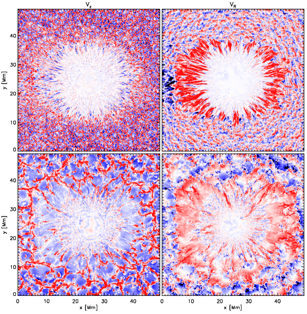
Figure 20.— Vertical (left) and radial (right) flow velocity at the $\tau=1$ level (top) and $3.4$ Mm depth (bottom). At the $\tau=1$ level ($3.4$ Mm depth) the vertical flow velocity is saturated at $3\,\mbox{km\,s}^{-1}$ ($0.8\,\mbox{km\,s}^{-1}$), the radial one at $6\,\mbox{km\,s}^{-1}$ ($0.8\,\mbox{km\,s}^{-1}$). While vertical motions in the penumbra are subdued compared to the surrounding granulation, horizontal flows clearly stand out. Horizontal outflows are strongest in the x-direction, where the nearby opposite polarity spots impose a more horizontal field. In contrast to the flow field in the photosphere radial motions do not stand as much over the surrounding convection cells and are also much less dependent on the position (x vs. y direction). The presence of the sunspot leads to a ring-like arrangement of convection cells around the spot. In contrast to the more or less randomly arranged convection cells at larger distance from the spot this preferred arrangement leads to the generation of mean flows with an amplitude comparable to convective flows at the given height.

6.3. Implications for simplified models

We address here only models that include driving processes for the Evershed flow, a more general discussion is presented in Sect. 8.

The picture presented above shows substantial differences to stationary siphon flow models that have been proposed to explain the Evershed flow. Those models assume that processes related to turbulent pumping near the outer edge of the penumbra (Montesinos & Thomas, 1997; Brummell et al., 2008) hold field lines down and establish the field line connectivity that allows then for siphon flows due to pressure differences between the inner and outer footpoint. We see stronger evidence in our simulation for a flow that is driven from within the penumbra regardless of the initial field line connectivity, even though siphon-like flow channels can result from this process in the outer penumbra (see, e.g., filament 5 in Fig. 19). Since we find fast outflows along horizontal stretches of field lines regardless of their field line connectivity we conjecture that siphon-like flow channels in the outer penumbra are more a consequence of the fast outflow than its cause.

This does not rule out additional contributions from processes as described by Montesinos & Thomas (1997) in the outer penumbra. The filament 6 we highlighted in Fig. 19 is a potential example for a siphon flow related to turbulent pumping near the edge of the penumbra. The footpoint in the outer penumbra is caused by a strong downdraft leading to an U-loop of field lines (see the upward returning flux in the left corner of the indicated sub domain). The outer footpoint of filament 6 has as a consequence fast downflows and low pressure (on average more than $10^{5}{\rm dyne}{\rm cm}^{-2}$ lower than the regions most of the field lines connect to further inward). We see a bundle of arch like field lines extending a few $100$ km above $\tau=1$ and having outflow velocities mostly in the $2-4\,\mbox{km\,s}^{-1}$ range (a few faster flows are found in the proximity of the footpoint), which is consistent with the predictions of most stationary siphon models. However, the flow velocities fall short of those present in filaments 2-5, where fast outflows are confined to almost horizontal stretches of the field lines in the deep photosphere over lengths of several Mm. When there are higher reaching arches present such as in filament 3 and 4, flow speeds are declining toward the highpoint, contrary to predictions from stationary siphon flow models.

The concentration of driving forces to a very narrow boundary layer beneath $\tau=1$ is not compatible with the acceleration of fluid along several Mm wide arches of field lines extending mostly above $\tau=1$.

Fast outflows in the deep photosphere are a natural outcome of the moving flux tube model (Schlichenmaier et al., 1998a, b) in which processes similar to convective overshoot limit the vertical rise of plasma. The fast outflows found there have been attributed in part to a hot upflow near the inner footpoint that is magnetically deflected outward and in part to horizontal pressure gradients resulting from radiative cooling. The former has some similarity to the magnetic ”deflection” we see in our magnetoconvection simulation leading to a process limited to a very narrow height range near $\tau=1$, but we do not see significant contributions from horizontal pressure gradients in the radial direction. The primary difference is that in the simplified flux tube picture there is only one inner footpoint present for the filament, while the driving process seen in our numerical simulation is approximately translation invariant along the filament, i.e. the entire filament is essentially a ”footpoint” in which this process accelerates fluid. The translation invariance also implies small contributions from horizontal pressure driving in the radial direction.

7. Deep flow component

Figure 21.— Vertical velocity and mass flux profile take at $R=18$ Mm in the outer penumbra (cf. Fig. 7). The solid line shows the radial flow velocity (scale on the left) and the dashed line the radial mass flux $v_{R}\varrho$ with the scale on the right. At a depth of $3$ Mm the deep flow component transports about $10$ times the mass of the Evershed flow due to the strong increase of mass density with depth.

In the previous section we focused on the driving of flows in the uppermost few $100$ km of the penumbra. While these flows can be primarily explained through strongly enhanced Lorentz force driving, there is no strong contribution present in more than $400$ km depth (cf. Fig. 12). The physical origin of this deeper reaching outflow becomes evident from Fig. 20. At the $\tau=1$ surface horizontal outflows stand out compared to typical granular flows at that height level, while vertical motions in the penumbra are subdued. Furthermore, strong outflows are found preferentially along the x-direction where the nearby opposite polarity spots impose a more horizontal magnetic field. In about $3.4$ Mm depth vertical and horizontal flows do not stand out in terms of amplitude, but rather in terms of the overall flow structure. In the periphery of the sunspot convection cells are arranged in a ring-like pattern in contrast to the random arrangement further away. This preferred arrangement leads to the appearance of large-scale mean flows (outflows away from the sunspot), which have amplitudes comparable to typical horizontal convective flows at the same depth, i.e. the flow amplitude should be a certain fraction of the rms velocity rather independent of depth as indicated in Fig. 7. While the appearance of an approximately axisymmetric mean flow is a consequence of geometric arrangement, the preferred outflow direction requires additional ingredients. A pure arrangement of convection cells in a ring-like fashion should lead to a pair of convection rolls, generating an inflow close to the spot and an outflow further out. A preference for the outflow can be a consequence of the presence of strong magnetic field in the center, which inhibits motions converging toward the spot but has less influence on the diverging motions further out. In addition large-scale pressure gradients can lead to the preference of outflows. We see in this simulation a combination of both. According to Fig. 12a) radial flows in the center penumbra are driven primarily by pressure forces in more than $300$ km depth. We see a preference for pressure driving of outflows, only a weak asymmetry is introduced by the Lorentz force, which opposes inflows more strongly than outflows. Note that most of the pressure driving originates from the region in between $R=16$ and $R=18$ Mm, where the deep flow component gains speed.

While the outflow close to $\tau=1$ clearly dominates in terms of flow velocity, the deep reaching flow component transports significantly more mass than the shallow Evershed flow. In Fig. 21, we compare vertical profiles of $\langle v_{R}\rangle$ and $\langle v_{R}\varrho\rangle$ at the position $R=18$ Mm in the outer penumbra. At a depth of $3$ Mm the mass flux is about $10$ times larger than the the mass flux of the Evershed flow in the photosphere. It is very likely that the deep flow component is related to large-scale moat flows observed around sunspots in the photosphere as well as deeper layers through helioseismology (see, e.g., Gizon & Birch (2005) for a recent review and references therein). To clearly establish this relationship we need however a numerical simulation covering a substantially longer time span as well as depth range, which is beyond this investigation.

8. Conclusions

We presented a detailed analysis of the recent numerical sunspot simulation by Rempel et al. (2009a). Our investigation focused on properties of penumbral fine structure near the $\tau=1$ level as well as the physical mechanisms behind the driving of large-scale outflows in sunspots at photospheric levels and beneath. Our main conclusions can be summarized as follows:

1. We find penumbral fine structure near $\tau=1$, which is compatible with the observationally inferred picture of an interlocking comb structure with fast $>8\,\mbox{km\,s}^{-1}$ Evershed flows along almost horizontal stretches of magnetic field.

2. Correlations between radial flow velocity, intensity, and field strength at the $\tau=1$ level show a good qualitative agreement with recent observations and are a direct consequence of convective energy transport in a sunspot penumbra.

3. The net contribution from large-scale flows to the mass and convective energy flux in the penumbra is found to be about $12-13\%$. Local contributions in the inner penumbra can reach $50\%$. Maintaining the penumbral brightness of $0.7L_{\odot}$ requires about $1\,\mbox{km\,s}^{-1}$ vertical rms velocity at the $\tau=1$ level.

4. We find in the sunspot penumbra two flow components, which we separate according to their scaling with respect to the convective rms velocity outside the penumbra ($v_{\rm rms}^{0}$). While the deep component (more than $500$ km beneath the photosphere) has an almost constant ratio to $v_{\rm rms}^{0}$ of about $50\%$ rather independent of depth, the shallow component (uppermost $500$ km) shows an increase toward the surface steeper than $v_{\rm rms}^{0}$. While the latter is essentially the Evershed flow, the former is likely related to a deep reaching moat flow component.

5. The near surface flow component is almost exclusively driven through the horizontal component of the Lorentz force along filaments. The energy for maintaining this flow is provided by vertical pressure forces in upflow regions, which are effectively deflected horizontally by an inclined magnetic field.

6. The Evershed flow is driven in a thin boundary layer beneath $\tau=1$. Essential ingredient is a strong vertical increase of $B_{R}$ beneath $\tau=1$ combined with a moderate vertical average field strength of a few $100$ G. The Evershed flow is strongly magnetized and reaches a peak velocity of about $|B_{R}|/\sqrt{4\pi\varrho}$ at $\tau=1$.

7. Upward advection of momentum and magnetic field by overturning convective motions in the penumbra is crucial for maintaining the conditions under which a quasi-stationary Evershed flow can be driven.

8. The deep reaching flow component results from a preferred geometric alignment of convection cells in the periphery of the sunspot. Asymmetries in pressure and Lorentz forces lead to a dominance of the outflow component. The flow amplitude is about $50\%$ of the convective rms velocity, rather independent of depth.

9. Flow channels cannot be easily identified with magnetic flux tubes. The field line connectivity is changing between inner and outer penumbra and we see no compelling evidence that the field line connectivity plays a major role in determining the Evershed flow speed; on the contrary, field line connectivity is established primarily as a consequence of the outflow.

A variety of simplified as well as magnetoconvective models for the penumbra have been discussed to explain the Evershed effect. The majority of the simplified models that have been used to describe the acceleration of horizontal flows in the penumbra is based on stationary or dynamic flux tube models.

We see strong limitations for the applicability of the thin flux tube approximation in the context of penumbral flow channels. The continuous mass exchange along flow channels due to overturning convective motions is not part of the flux tube picture (it is essentially orthogonal to the assumptions), but found to be substantial in the presented numerical simulation. In addition the changing field line connectivity along the flow channels from inner to outer penumbra does not allow for an easy identification with a flux tube, at least not for the whole length of it. It is in general difficult to find meaningful compact footpoints that are representative of the field in inner and outer penumbra at the same time.

We see limitations for the applicability of stationary flux tube models such as Meyer & Schmidt (1968); Thomas (1988); Degenhardt (1989, 1991); Thomas & Montesinos (1993); Montesinos & Thomas (1997) as explanation for the flows in our simulation. Both, field line connectivity and the causality between outflows and field line connectivity point toward processes in which the conditions in the outer footpoint (if it exists at all) are of minor influence on the flow pattern and outflows are mostly driven by convective motions within the penumbra. In addition fast outflows are found preferentially in the deep photosphere along almost horizontal stretches of field lines regardless of their connectivity, which is different from the situation described in most stationary siphon models to date. This does not rule out additional contributions in the outer penumbra from processes similar to those described in Montesinos & Thomas (1997), where turbulent pumping by convective motions at the periphery of the penumbra plays a crucial role in establishing the field geometry. Filament 6 in Fig. 19 is one possible example for such a configuration. Note that our simulation might not be fully representative of a ”typical” outer penumbra due to the setup with a nearby opposite polarity spot, even though, the combination of strong horizontal field in between both sunspots with a strong downflow lane due to the converging Evershed flows from both sides has a tendency to enhance submergence of field by convective motions.

The moving flux tube model of Schlichenmaier et al. (1998a, b) naturally produces outflows located in the deep photosphere and similarly to the situation in our simulation most driving is focused on the inner footpoint. The acceleration of outflows is attributed to a combination of ”deflection” of hot upflows and horizontal pressure gradients resulting from radiative cooling. In contrast to moving flux tube models we see in our simulation strong limits on the overall role horizontal pressure driving plays for the acceleration of plasma in the radial direction, while the magnetic ”deflection” of hot upflows is not restricted to the inner footpoint but found everywhere throughout the penumbra.

Recently Thomas (2010) and also Priest (2010, private communication) have suggested that flows in the penumbra could be described in terms of “dynamical” siphon models, in which pressure gradients are produced by MHD processes such as magnetoconvection and these drive time-dependent flows along the magnetic field, which then reacts by Lorentz forces to the presence of the flow: in this view, field line connectivity plays only a secondary role and is more a consequence than a cause. While describing part of the picture, however, one also needs to understand the fluid motions that are responsible for the filamentation and most of the energy transport. Furthermore, we showed that the magnetic driving of outflows originates from narrow boundary layers that form beneath $\tau=1$ in regions where convective upflows are present. These regions arise as a consequence of magnetoconvection and are not captured by flux tube models that do not include a filament sub-structure and overturning convection.

Galloway (1975) presented a phenomenological model based on the ”roll-convection” picture introduced by Danielson (1961), which explains the Evershed flow as a consequence of unbalanced horizontal Lorentz force components: while the Lorentz force balances the gas pressure deficit of the sunspot on average, the filamentation of the penumbra implies a strong azimuthal variation and therefore a violation of this balance locally that is responsible for driving the Evershed flow. It is argued further that the Evershed flow is located in dark filaments, where downward directed motions concentrate magnetic field and lead in return to an above average Lorentz force. While our magnetoconvection simulation certainly produces a Lorentz force that is strongly varying in the azimuthal direction, our results disagree with Galloway (1975) in detail as we find that most of the Evershed flow is driven in upflow regions.

Several other penumbra models focus on the fine structure of the penumbra, without necessarily addressing the driving of large-scale outflows. One of these models which has gotten a lot of attention recently is the ”gappy” penumbra model by Spruit & Scharmer (2006); Scharmer & Spruit (2006). In its original form this model proposed essentially field free upflow plumes embedded in an inclined background field. While this structure certainly captures the essence of the convective picture seen in the numerical simulations presented here, there has been a lot of discussion of how field free these ”gaps” really are and to which extent the field strength seen in present simulations is affected by numerical diffusion (see, e.g., discussion in Nordlund & Scharmer, 2010). The physical explanation of the Evershed flow presented here implies the presence of strong Lorentz forces in the uppermost few $100$ km beneath the $\tau=1$ level in the penumbra, which requires the presence of strong $1-2$ kG magnetic field. In that sense our results are incompatible with models that predict field free gaps at photospheric levels! Furthermore we do not see evidence that the field structure is heavily influenced by numerical dissipation as the analysis presented in the bottom panels of Fig. 16 reveals. Also it remains very controversial whether the wealth of spectropolarimetric observations could be explained by an essentially unmagnetized Evershed flow (see, e.g., Thomas, 2010). Nevertheless, the results presented here indicate an almost Salomonian solution to this discussion: Strong field is confined to a narrow boundary layer just beneath $\tau=1$, while further down the field strength is substantially reduced compared to the ambient plasma (but still of the order of $1$ kG). This scenario was also brought forward as a possible solution for this problem in a recent review by Scharmer (2009).

Recently a variety of different magnetoconvection simulations with radiative transfer such as Heinemann et al. (2007); Rempel et al. (2009b); Kitiashvili et al. (2009) have been used to model the penumbra. The models by Heinemann et al. (2007) and Rempel et al. (2009b) focused primarily on the transition from umbra toward inner penumbra, which corresponds roughly to the innermost edge of the region we analyzed in this investigation. The energy conversion terms for that region are displayed in Fig. 14 and do not show (except for the overall amplitude) a fundamental difference to Fig. 11. From this we conclude that the driving mechanisms for horizontal outflows in Heinemann et al. (2007) and Rempel et al. (2009b) is essentially the same as discussed here. The overall picture we described in Sect. 6 is similar to Scharmer et al. (2008). Kitiashvili et al. (2009) studied in an idealized setup the influence of field strength and inclination on large-scale flows and found a strong dependence of outflow speeds on the average inclination and field strength, which is consistent with the mechanism explained here. They also reported on temporal variations of the Evershed flow speed on timescales of $15$ to $40$ minutes.

Our analysis essentially reinforces conclusions of Scharmer et al. (2008); Rempel et al. (2009a) that the penumbra is anisotropic magnetoconvection and that the Evershed flow can be understood as convective flow component in the direction of the magnetic field. The similarity between plage region and penumbra with respect to the different terms in the kinetic energy equation (Fig. 9) is quite astonishing, a comparison between the depth profiles of rms velocities points toward anisotropy as the main difference (see Rempel et al. (2009a), supporting online material). Nevertheless, there are also notable differences which clearly differentiate the Evershed flow from horizontal flows in typical convection. While the latter is entirely pressure driven, the Evershed flow is almost completely Lorentz force driven. Only flows that turn over laterally in penumbral filaments remain pressure driven. In addition pressure/buoyancy driving takes place primarily in upflow regions, in contrast to field free convection that is driven by top heavy downflow regions. An interesting new aspect pointed out in this paper is the confinement of the underlying driving mechanism to very narrow boundary layers that exist just beneath $\tau=1$.

For clarification we want point out that the driving of the Evershed flow is achieved through the radial component of the Lorentz force while the total work done by Lorentz forces remains negative, i.e. the net effect is a sink for kinetic energy. The overall underlying energy source is convective instability, which enters the kinetic energy balance through pressure/buoyancy driving. The Lorentz force facilitates the energy exchange between the pressure driving in the vertical direction and the horizontal Evershed flow acceleration. A necessary condition for the latter is the shift of pressure/buoyancy driving from downflow to upflow regions in the penumbra we described above.

In addition to the mechanism leading to the fast Evershed flow in the upper most few $100$ km of a sunspot penumbra we have also identified a mechanism leading to the formation of a larger scale outflow in deeper layers. In contrast to the Evershed flow the deeper flow scales proportional to the convective rms velocity (outside the sunspot), the dominant radial outflow reaches typically amplitudes $\sim 0.5\,v_{\rm rms}$. The main reason for this flow cell is a preferred circular alignment of convection cells surrounding the sunspot. As a consequence the azimuthal average over this ring-like pattern of convection cells does not vanish and leads to mean flow speeds scaling proportional to $v_{\rm rms}$. A preference for the outflow results from a combination of pressure and Lorentz forces. While this flow does not stand out in terms of flow velocity as the Evershed flow, the radial mass flux is substantially larger, which make a connection with the large-scale moat flows observed around sunspots likely. In this simulation we do not see evidence for a converging collar flow that was found previously in 2D axisymmetric simulations (Hurlburt & Rucklidge, 2000; Botha et al., 2006, 2008). In a future publication we will investigate the subsurface structure of this flow component in deeper domains and evolution over timescales longer than those covered by the numerical simulation presented here.

The deep flow component described in Sect. 21 should be in principle observable through local helioseismology. The clear prediction is here an outflow of plasma with an amplitude of about $50\%$ of the convective rms velocity reaching downward several Mm beneath the penumbra. This result is in contradiction with some recent helioseismic inversions such as Zhao et al. (2001, 2010), which point toward an inflow in a depth range from $1.5$ to $5$ Mm. One the other hand Gizon et al. (2009) reported on an outflow over the uppermost $5$ Mm.

While most of the processes responsible for driving the Evershed flow are located beneath the $\tau=1$ level, there are nevertheless several aspects of the magnetoconvective penumbra model presented here that can be constrained through observations. As presented in Sect. 3 most of the energy is transported in the penumbra by laterally overturning convective motions. We find a very tight relationship between intensity and vertical rms velocity of the form $I\propto\sqrt{v_{z\,rms}(\tau=1)}$. From this follows that the vertical rms velocity at $\tau=1$ in the penumbra with $I\approx 0.7I_{\odot}$ should be about half of the value found in the quiet sun, i.e. about 1 $\mbox{km\,s}^{-1}$. This value is consistent with the recent findings of Franz & Schlichenmaier (2009), who computed from Hinode observations velocity distributions functions for both quiet Sun and penumbra (see Fig.3 in their paper). The half width at half maximum of the vertical velocity distribution function for the penumbra is about $500\,\mbox{m\,s}^{-1}$, while the same analysis results in $1\,\mbox{km\,s}^{-1}$ for the quiet Sun, i.e. the latter falls short by about a factor of $2$ compared to the value we find for the quiet Sun at $\tau=1$ (due to a combination of limited observational resolution as well as the sharp decline of $v_{z}$ above $\tau=1$). If we assume that the same shortfall applies also to the penumbra, the vertical velocity structure reported in Franz & Schlichenmaier (2009) is at least in a statistical sense fully consistent with the amount of overturning convection we see in the numerical simulation presented here. Other consequences of the magnetoconvective model are the sign changes in the $I-v_{R}$ and $B-v_{R}$ correlations presented in Fig. 4. They are consistent with the analysis of Hinode data presented by Ichimoto et al. (2007a) (see Fig. 3 therein). A positive $B-v_{R}$ correlation in the outer penumbra was suggested by Tritschler et al. (2007) and Ichimoto et al. (2008) based on observations of the net circular polarization (NCP) at different viewing angles. As explained in Sect. 5 the observable consequences of the Evershed flow driving mechanism are a moderate increase of $B_{R}$ and a steep increase of $v_{R}$ toward $\tau=1$. $v_{z}$ shows a very steep gradient in the deep photosphere. The peak velocity of the Evershed flow in the deep photosphere should be around $|B_{R}|/\sqrt{4\pi\varrho}$.

The fact that the simulated Evershed flow is a deep photospheric flow is a direct consequence of its convective origin. On the observational side the depth dependence of the Evershed flow is debated. While the investigations by Rimmele (1995) and Stanchfield et al. (1997) point toward flows in elevated flow channels, recent work by Schlichenmaier et al. (2004), Bellot Rubio et al. (2006), and Borrero et al. (2008) is in support of a flow in the deep photosphere declining with height. Another point heavily debated is the presence or absence of overturning convection in the penumbra. Support for overturning convection is found by Ichimoto et al. (2007b); Zakharov et al. (2008); Rimmele (2008); Bharti et al. (2010), while Bellot Rubio et al. (2005); Ichimoto et al. (2007a); Franz & Schlichenmaier (2009); Bellot Rubio et al. (2010) see primarily support for Evershed flow related upflows in the inner and downflows in the outer penumbra – a flow pattern that accounts in our model only for a small fraction of the unsigned mass and energy flux integrated over the penumbra. It appears that overcoming the discrepancy between the presence of overturning convection in MHD simulations and the lack of evidence in many high resolution observations is one of the biggest challenges both numerical models and observations will face in the future. It is unlikely that the absence of overturning convection is the solution to this discrepancy; a brightness of $0.7I_{\odot}$ or more requires overturning mass flux at a level not much less than granulation. An other possible solution could be related to thin boundary layers, which are indicated but not well resolved in the simulation presented here. If quantities such as flow velocities and magnetic field change dramatically over short distances, moving a $\tau$-surface by a distance comparable to our grid spacing can make a dramatic differences for the visibility of such feature. This clearly indicates that the simulation presented here can only be considered as a first step in that direction.

A convergence study of the properties highlighted in this investigation covering the resolution range from $96\times 32$ to $16\times 12$ km resolution (horizontal $\times$ vertical) is in progress. A preliminary analysis shows that most magnetoconvective properties of the penumbra are robust (qualitative agreement over the whole range investigated, quantitative agreement from $48\times 24$ km resolution upward), while the photospheric appearance of sunspot fine structure improves substantially with resolution. The currently highest resolution case is presented in Rempel (2010).

References

- Bellot Rubio et al. (2005) Bellot Rubio, L. R., Langhans, K., & Schlichenmaier, R. 2005, A&A, 443, L7
- Bellot Rubio et al. (2010) Bellot Rubio, L. R., Schlichenmaier, R., & Langhans, K. 2010, ApJ, 725, 11
- Bellot Rubio et al. (2006) Bellot Rubio, L. R., Schlichenmaier, R., & Tritschler, A. 2006, A&A, 453, 1117
- Bharti et al. (2010) Bharti, L., Solanki, S. K., & Hirzberger, J. 2010, ApJ, 722, L194
- Borrero et al. (2008) Borrero, J. M., Lites, B. W., & Solanki, S. K. 2008, A&A, 481, L13
- Botha et al. (2008) Botha, G. J. J., Busse, F. H., Hurlburt, N. E., & Rucklidge, A. M. 2008, MNRAS, 387, 1445
- Botha et al. (2006) Botha, G. J. J., Rucklidge, A. M., & Hurlburt, N. E. 2006, MNRAS, 369, 1611
- Brummell et al. (2008) Brummell, N. H., Tobias, S. M., Thomas, J. H., & Weiss, N. O. 2008, ApJ, 686, 1454
- Cabrera Solana et al. (2007) Cabrera Solana, D., Bellot Rubio, L. R., Beck, C., & Del Toro Iniesta, J. C. 2007, A&A, 475, 1067
- Clyne et al. (2007) Clyne, J., Mininni, P., Norton, A., & Rast, M. 2007, New Journal of Physics, 9, 301
- Clyne & Rast (2005) Clyne, J. & Rast, M. 2005, in Society of Photo-Optical Instrumentation Engineers (SPIE) Conference Series, Vol. 5669, Society of Photo-Optical Instrumentation Engineers (SPIE) Conference Series, ed. R. F. Erbacher, J. C. Roberts, M. T. Gröhn, & K. Börner , 284–294
- Danielson (1961) Danielson, R. E. 1961, ApJ, 134, 289
- Degenhardt (1989) Degenhardt, D. 1989, A&A, 222, 297
- Degenhardt (1991) —. 1991, A&A, 248, 637
- del Toro Iniesta et al. (2001) del Toro Iniesta, J. C., Bellot Rubio, L. R., & Collados, M. 2001, ApJ, 549, L139
- Dialetis et al. (1985) Dialetis, D., Mein, P., & Alissandrakis, C. E. 1985, A&A, 147, 93
- Evershed (1909) Evershed, J. 1909, MNRAS, 69, 454
- Franz & Schlichenmaier (2009) Franz, M. & Schlichenmaier, R. 2009, A&A, 508, 1453
- Galloway (1975) Galloway, D. J. 1975, Sol. Phys., 44, 409
- Gizon & Birch (2005) Gizon, L. & Birch, A. C. 2005, Living Reviews in Solar Physics, 2, 6
- Gizon et al. (2009) Gizon, L., Schunker, H., Baldner, C. S., Basu, S., Birch, A. C., Bogart, R. S., Braun, D. C., Cameron, R., Duvall, T. L., Hanasoge, S. M., Jackiewicz, J., Roth, M., Stahn, T., Thompson, M. J., & Zharkov, S. 2009, Space Sci. Rev., 144, 249
- Grosser (1991) Grosser, H. 1991, Zur Entstehung der Penumbra-Filamentierung von Sonnenflecken durch die Wirkung von Konvektionsrollen, PhD thesis, Universität Göttingen
- Heinemann et al. (2007) Heinemann, T., Nordlund, Å., Scharmer, G. B., & Spruit, H. C. 2007, ApJ, 669, 1390
- Hurlburt et al. (1996) Hurlburt, N. E., Matthews, P. C., & Proctor, M. R. E. 1996, ApJ, 457, 933
- Hurlburt et al. (2000) Hurlburt, N. E., Matthews, P. C., & Rucklidge, A. M. 2000, Sol. Phys., 192, 109
- Hurlburt & Rucklidge (2000) Hurlburt, N. E. & Rucklidge, A. M. 2000, MNRAS, 314, 793
- Ichimoto et al. (2007a) Ichimoto, K., Shine, R. A., Lites, B., Kubo, M., Shimizu, T., Suematsu, Y., Tsuneta, S., Katsukawa, Y., Tarbell, T. D., Title, A. M., Nagata, S., Yokoyama, T., & Shimojo, M. 2007a, PASJ, 59, 593
- Ichimoto et al. (2007b) Ichimoto, K., Suematsu, Y., Tsuneta, S., Katsukawa, Y., Shimizu, T., Shine, R. A., Tarbell, T. D., Title, A. M., Lites, B. W., Kubo, M., & Nagata, S. 2007b, Science, 318, 1597
- Ichimoto et al. (2008) Ichimoto, K., Tsuneta, S., Suematsu, Y., Katsukawa, Y., Shimizu, T., Lites, B. W., Kubo, M., Tarbell, T. D., Shine, R. A., Title, A. M., & Nagata, S. 2008, A&A, 481, L9
- Kitiashvili et al. (2009) Kitiashvili, I. N., Kosovichev, A. G., Wray, A. A., & Mansour, N. N. 2009, ApJ, 700, L178
- Langhans et al. (2007) Langhans, K., Scharmer, G. B., Kiselman, D., & Löfdahl, M. G. 2007, A&A, 464, 763
- Langhans et al. (2005) Langhans, K., Scharmer, G. B., Kiselman, D., Löfdahl, M. G., & Berger, T. E. 2005, A&A, 436, 1087
- Meyer & Schmidt (1968) Meyer, F. & Schmidt, H. U. 1968, Zeitschrift Angewandte Mathematik und Mechanik, 48, 218
- Montesinos & Thomas (1997) Montesinos, B. & Thomas, J. H. 1997, Nature, 390, 485
- Nordlund & Scharmer (2010) Nordlund, Å. & Scharmer, G. B. 2010, in Magnetic Coupling between the Interior and Atmosphere of the Sun, ed. S. S. Hasan & R. J. Rutten, 243–254
- Ortiz et al. (2010) Ortiz, A., Bellot Rubio, L. R., & Rouppe van der Voort, L. 2010, ApJ, 713, 1282
- Rempel (2010) Rempel, M. 2010, IAU Symp. 273, arXiv:1011.0981
- Rempel et al. (2009a) Rempel, M., Schüssler, M., Cameron, R. H., & Knölker, M. 2009a, Science, 325, 171
- Rempel et al. (2009b) Rempel, M., Schüssler, M., & Knölker, M. 2009b, ApJ, 691, 640
- Riethmüller et al. (2008) Riethmüller, T. L., Solanki, S. K., & Lagg, A. 2008, ApJ, 678, L157
- Rimmele (2008) Rimmele, T. 2008, ApJ, 672, 684
- Rimmele & Marino (2006) Rimmele, T. & Marino, J. 2006, ApJ, 646, 593
- Rimmele (1994) Rimmele, T. R. 1994, A&A, 290, 972
- Rimmele (1995) —. 1995, A&A, 298, 260
- Scharmer (2009) Scharmer, G. B. 2009, Space Sci. Rev., 144, 229
- Scharmer et al. (2002) Scharmer, G. B., Gudiksen, B. V., Kiselman, D., Löfdahl, M. G., & Rouppe van der Voort, L. H. M. 2002, Nature, 420, 151
- Scharmer et al. (2007) Scharmer, G. B., Langhans, K., Kiselman, D., & Löfdahl, M. G. 2007, in Astronomical Society of the Pacific Conference Series, Vol. 369, New Solar Physics with Solar-B Mission, ed. K. Shibata, S. Nagata, & T. Sakurai, 71–+
- Scharmer et al. (2008) Scharmer, G. B., Nordlund, Å., & Heinemann, T. 2008, ApJ, 677, L149
- Scharmer & Spruit (2006) Scharmer, G. B. & Spruit, H. C. 2006, A&A, 460, 605
- Schlichenmaier et al. (2005) Schlichenmaier, R., Bellot Rubio, L. R., & Tritscher, A. 2005, Astronomische Nachrichten, 326, 301
- Schlichenmaier et al. (2004) Schlichenmaier, R., Bellot Rubio, L. R., & Tritschler, A. 2004, A&A, 415, 731
- Schlichenmaier et al. (1998a) Schlichenmaier, R., Jahn, K., & Schmidt, H. U. 1998a, ApJ, 493, L121
- Schlichenmaier et al. (1998b) —. 1998b, A&A, 337, 897
- Schüssler & Vögler (2006) Schüssler, M. & Vögler, A. 2006, ApJ, 641, L73
- Shine et al. (1994) Shine, R. A., Title, A. M., Tarbell, T. D., Smith, K., Frank, Z. A., & Scharmer, G. 1994, ApJ, 430, 413
- Sobotka & Jurčák (2009) Sobotka, M. & Jurčák, J. 2009, ApJ, 694, 1080
- Socas-Navarro et al. (2004) Socas-Navarro, H., Pillet, V. M., Sobotka, M., & Vázquez, M. 2004, ApJ, 614, 448
- Solanki (2003) Solanki, S. K. 2003, A&Ar, 11, 153
- Solanki & Montavon (1993) Solanki, S. K. & Montavon, C. A. P. 1993, A&A, 275, 283
- Spruit & Scharmer (2006) Spruit, H. C. & Scharmer, G. B. 2006, A&A, 447, 343
- Stanchfield et al. (1997) Stanchfield, II, D. C. H., Thomas, J. H., & Lites, B. W. 1997, ApJ, 477, 485
- Thomas (1988) Thomas, J. H. 1988, ApJ, 333, 407
- Thomas (2010) Thomas, J. H. 2010, in Magnetic Coupling between the Interior and Atmosphere of the Sun, ed. S. S. Hasan & R. J. Rutten, 229–242
- Thomas & Montesinos (1993) Thomas, J. H. & Montesinos, B. 1993, ApJ, 407, 398
- Thomas & Weiss (1992) Thomas, J. H. & Weiss, N. O. 1992, in Sunspots: Theory and Observations, ed. J. H. Thomas & N. O. Weiss (Kluwer, NATO ASI, C 375), 3–59
- Thomas & Weiss (2004) Thomas, J. H. & Weiss, N. O. 2004, ARA&A, 42, 517
- Thomas & Weiss (2008) —. 2008, Sunspots and Starspots, ed. Thomas, J. H. & Weiss, N. O. (Cambridge University Press)
- Tritschler et al. (2007) Tritschler, A., Müller, D. A. N., Schlichenmaier, R., & Hagenaar, H. J. 2007, ApJ, 671, L85
- Vasil & Brummell (2009) Vasil, G. M. & Brummell, N. H. 2009, ApJ, 690, 783
- Wentzel (1992) Wentzel, D. G. 1992, ApJ, 388, 211
- Westendorp Plaza et al. (2001) Westendorp Plaza, C., del Toro Iniesta, J. C., Ruiz Cobo, B., & Martínez Pillet, V. 2001, ApJ, 547, 1148
- Zakharov et al. (2008) Zakharov, V., Hirzberger, J., Riethmüller, T. L., Solanki, S. K., & Kobel, P. 2008, A&A, 488, L17
- Zhao et al. (2001) Zhao, J., Kosovichev, A. G., & Duvall, T. L. 2001, ApJ, 557, 384
- Zhao et al. (2010) Zhao, J., Kosovichev, A. G., & Sekii, T. 2010, ApJ, 708, 304