Polarization transitions in Quantum Dot Quantum Well Arrays

Abstract

With the improvement in fabrication techniques it is now possible to produce atom-like semiconductor structures with unique electronic properties. This makes possible periodic arrays of nano-structures in which the Coulomb interaction, polarizability, and tunneling may all be varied. We study the collective properties of 2D arrays and 3D face centered cubic lattices of singly-charged nano-spherical shells, sometimes called ‘quantum-dot quantum wells’ or ‘core-shell quantum dots.’ We find that for square arrays, the classical groundstate is an Ising anti-ferroelectret (AFE), while the quantum groundstate undergoes a transition from a uniform state to an AFE. The triangular lattice, in contrast, displays properties characteristic of frustration. Three dimensional face-centered cubic lattices polarize in planes, with each layer alternating in direction. We discuss the possible experimental signals of these transitions.

I Introduction

With improvements in the colloidal fabrication of structures on the micro- and nanometer scale, new areas of study have been made possible. In particular, researchers are now able to produce atom-like electronic devices with their own unique spectra and shell structures ph ; pengdots . The distinct characteristics of such devices may be controlled through fabrication, in turn producing structures with unique electronic properties.

Periodic arrays of atoms have been studied extensively for nearly a century. However, we may now examine periodic arrays of nano-structures in which the tunneling, polarizability, and Coulomb interaction may all be varied, thus giving us the power to control an electronic wavefunction to a degree without an atomic analogue. Small multi-dot systems show coherent phenomena in experimentsmultidot while disordered arrays of colloidal quantum dots display variable long-range hopping.hop It should soon be possible to examine collective electronic excitations of periodic nanostructures. With this in mind, we choose a nano-structure which will confine the electron on the nanoscale in such a way as to bring about novel characteristics.

In this paper we consider electrons confined to spherical shells, sometimes called “quantum dot quantum wells” (QDQW) or “core-shell quantum dots.” QDQWs are heterostructures where layers of different semi-conducting materials alternate in a single nano-crystal. One well characterized example is the CdS/CdSe/CdS system, i.e. a CdS core and outer shell with a CdSe inner shell b . In this case each layer is on the order of 1-2 nm and is separated by a large electronic band gap, thus allowing the investigation of quantum confinement in a geometry in which electrons occupy the surface of a sphere. CdS/CdSe/CdS QDQW’s have also been found to have an electron-g factor which varies as a function of quantum well width as well as a transverse spin lifetime of several nano-seconds at temperatures approaching room temperature b .

We choose QDQW’s for two reasons. First, because they have already be fabricated and are well-characterized,b and second, because their excluded core structure yields properties not found in regular quantum dot systems. Previous researchrings has found that in a 1D array of singly-charged nano-rings, a quantum phase transition ($T=0$) occurs which allows the system to spontaneously break symmetry into anti-ferroeletric (AFE) alignment. Studies of the 2D ring problem revealed another phase transition from random orientation to a striped AFE state, analogous to unitary transition of the 2D XY model. The focus of this paper is to show an analogous transition occurs in an ordered array of QDQW’s.

In the section below we describe our model, and then our methods for analyzing it in the classical and quantum mechanical limits. We then present results for the 2D square lattice, the 2D triangular lattice and the 3D face-centered cubic (FCC) lattice. Both the 2D square lattice and 3D face-centered cubic lattice systems yield a phase transition from random (classical) or uniform (quantum mechanical) distribution to an anti-ferroelectric state.

II The Model

In our model, each QDQW is treated as a infinitesimally thick spherical shell of radius $R$ with an electric charge on the surface. Charging might be achieved either by doping,ddots tunneling from a backgateor be adjusting an electrochemical potential.hop The radial degree of freedom can be neglected when the gap between radial excitations is large compared to that of orbital eigenstates. We then consider periodic arrays of singly-charged QDQW’s in either two or three dimensions and define a distance, $D$, between neighbors. In 2D we choose $D$ as the lattice constant so that $D>2R$. In a 3D face-centered cubic lattice $D$ is half the distance between vertices of the FCC cells so that the separation between nearest neighbors is given by $\sqrt{2}D$. We then consider the electrostatic interaction solely between nearest neighbors. Though the Coulomb repulsion acts over large distances, we assume that there is sufficient screening so that only nearest neighbor interactions are significant. Furthermore, the insulating shell around each QDQW allows us to ignore electron tunneling between dots.

II.1 Classical Analysis

Before solving a quantum mechanical problem it is often helpful to look at the classical case, which is usually easier to solve and provides an guide to the quantum ground state. Classically the electron is a point charge constrained to the surface of a sphere. Because of this constraint, it has a dipole moment (with respect to the shell center) of constant magnitude but random direction. Adjacent moments interact leading to the polarization instability, as we will show below.

There is only one energy scale in the classical problem, the Coulomb energy $E_{c}=e^{2}/D$. The electrostatic energy of the array is given by

$$U=\sum_{i,j\in n.n.\atop i\neq j}^{N}{e^{2}\over|{\vec{r}}_{i}(\theta_{i},\phi_{i})-{\vec{r}}_{j}(\theta_{j},\phi_{j})|}U={1\over 2}\sum_{i,j\in n.n.}^{N}{e^{2}\over|{\vec{r}}_{i}-{\vec{r}}_{j}|}$$ (1)

where $\vec{r}_{i}$ is the location of the $i$-th electron, $i$ and $j$ are restricted to nearest neighbors, and the factor of $1/2$ corrects for double counting. We define the expansion parameter $\epsilon\equiv R/D$ and expand the potential to second order:

$$U/E_{c} \approx U_{2}\equiv{1\over 2}\sum_{i,j\in n.n.}\left\{(1+\epsilon^{2})\right.$$ (2)

$$+ \left.\epsilon^{2}\left[{\vec{s}}_{i}\cdot{\vec{s}}_{j}+{3\over 2}({\hat{D}_{i,j}}\cdot({\vec{s}}_{i}-{\vec{s}}_{j}))^{2}\right]\right\}.$$

where $E_{c}\equiv e^{2}/D$ is a measure of the Coulomb interaction between shells. Here we specify the position of each charge by a unit vector ${\vec{s}}_{i}$ pointing from the center of the $i$-th sphere to the charge on that sphere. The unit vector ${\hat{D}_{i,j}}$ points from the center of the $i$-th to the center of the $j$-th sphere. We have also assumed that the lattice possesses reflection symmetry. From eq.(2) we see that the system has an AFE Heisenberg interaction and a symmetry breaking term. The symmetry breaking term encourages alignment of adjacent spins in the direction of the lattice vector connecting them. Further analysis requires knowledge of the lattice vectors of the specific system.

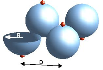
Figure 1: A schematic picture of the groundstate of classical point electrons in a 2D array of spherical shells. Each shell is of radius R and separated from its neighbor by a distance D. The 2D ordering is antiferroelectric for the infinite system size.

II.2 Quantum Mechanical Analysis

Instead of a single point charge on a sphere, in the quantum mechanical problem the electron is treated as a charge distribution constrained to the surface of a spherical shell. We now have two competing energy terms: the kinetic, which aims to spread the wave function, and the potential, which is strictly the Coulomb interaction between nearest neighbors. Our starting Hamiltonian is $H=T+U$ where the kinetic energy is given by:

$$T = -{E_{q}}\,\sum_{i}\,{1\over\sin{\theta_{i}}}{\partial\over\partial\theta_{i}}{1\over\sin{\theta_{i}}}{\partial\over\partial\theta_{i}}+{1\over\sin^{2}{\theta_{i}}}{\partial^{2}\over\partial\phi_{i}^{2}}$$ (3)

$$= -{E_{q}}\sum_{i}\nabla^{2}_{\Omega_{i}}\hfill$$ (4)

where $E_{q}\equiv{\hbar^{2}/2m^{*}R^{2}}$, and $m^{*}$ is the effective mass of the electron. In moving to angular variables, we write the unit vectors in eq(2) in terms of angle variables, $\vec{s}_{i}=\sin{\theta_{i}}\cos{\phi_{i}}\,\hat{x}+\sin{\theta_{i}}\sin{\phi_{i}}\,\hat{y}+\cos{\theta_{i}}\,\hat{z}$. If we measure our energy in units of $E_{q}$, our scaled Schrodinger equation is then

$$\left(\sum_{i}\nabla_{\Omega_{i}}^{2}+\lambda\,U\right)\psi=\tilde{E}\,\psi$$ (5)

where $\lambda$ is the ratio between the Coloumb and confinement energies, $\lambda={E_{c}/E_{q}}$ and $\tilde{E}$ is the dimensionless energy.

We calculate the groundstate using a variational approximation. For the $i$-th ring we choose a variational wave function, using only the first four spherical harmonics ($Y_{\ell m}$):

$$\psi_{\rm var}(\theta_{i},\phi_{i};\alpha_{i};\beta_{i},\gamma_{i})=\cos(\beta_{i})Y_{00}+\sin(\beta_{i})\cos(\alpha_{i})Y_{10}$$

$$+\sin(\beta_{i})\sin(\alpha_{i})\sqrt{3\over 2\pi}\sin(\theta_{i})\cos(\phi_{i}-\gamma_{i})$$ (6)

where we have used time reversal symmetry to force the wave function to be real. We are able to use this form since at low energies, each electron will occupy one of the lowest energy states. Even at full polarization the charge is not strongly localized; this is demonstrated in fig.(2) If the system will not polarize in this approximation, it will not be able to do so if we include higher energy states. This is done for a unit cell that respects the periodicity found in the classical simulations. Separation between neighbors is assumed to be sufficiently large to neglect tunneling effects and enable the use of the Hartree approximation.

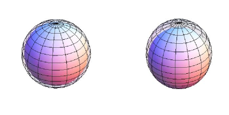
Figure 2: Spherical plot showing the charge polarization of a single lattice site for the 2D square array. Left is a uniform surface charge density ($1/4\pi$) represented by a mesh sphere of radius $1+1/4\pi$ surrounding a solid sphere of unit radius. Right is a plot of the polarized charge density, again represented by a spherical mesh with a radius $1+\psi^{2}$ surrounding a solid sphere of unit radius. The charge is not strongly localized since we are dealing with only the lowest spherical harmonics. Nearest neighbors display the same behavior but with opposite polarization.

III 2D Square Lattice

We first analyze the 2D square lattice assuming periodic boundary conditions. Below we present the classical and quantum mechanical analyses.

III.1 Classical Phase Transition

The nature of the symmetry breaking term in the square lattice can be clarified by resolving the interaction into components:

$$U_{2} = {1\over 2}\left\{2\sum_{i}\left(1+2\epsilon^{2}\right)-{3\epsilon^{2}}(s_{i}^{z})^{2}\right.$$ (7)

$$+ \left.\sum_{i,j\in n.n.}\epsilon^{2}\left[-2{\vec{s}}_{i}\cdot{\vec{s}}_{j}+3s_{i}^{(z)}s_{j}^{(z)}\right]\right\}.$$

The first term is an irrelevant constant; the second term breaks the rotational symmetry, favoring spins aligned along the z-axis. The third term is a Heisenberg ferroelectric coupling while the last and larger term is an Ising antiferroelectric coupling. An AFE state, when possible, will maximize the second and fourth terms, minimizing the total energy. This is confirmed by Monte Carlo analysis.

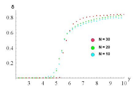
Figure 3: A plot of the classical phase transition from random alignment to the anti-ferroelectric (AFE) state Fig. (1) through $\gamma\equiv\beta E_{c}$, a measure of interaction strength, at zero temperature. Here $\delta$ is a measure of the system’s AFE order. Systems are square with periodic boundaries of size N=10, N=20, and N=30 and have $R/D=0.417$. Larger system sizes have sharper transitions.

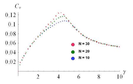
Figure 4: A plot of the heat capacity when $R/D=0.417$ for N=10, N=20, and N=30 against $\gamma\equiv\beta E_{c}$, a measure of interaction strength. Here $C_{v}$ is the system’s heat capacity. For larger system sizes, the peak around the transition point is sharper.

Monte Carlomc simulations were performed on 10$\times$10, 20$\times$20 and 30$\times$30 arrays. The low temperature ($e^{2}/kTD)>>1$) configuration is an antiferroelectric (AFE) pattern, Fig. (1). Furthermore, a phase transition from the unordered state to an AFE aligned state was found numerically. The transition is Ising-like, with a discontinuous change in the staggered polarization and a peak in the specific heat which is expected to sharpen into a divergence as the system size is increased. The value of the temperature at the peak extrapolates to $kT_{c}=XXX$ for an infinite size system, which should be compared to the expected value of $2.24$ for the 2D Ising model.huang

We can expand about the minimum energy state in order to calculate the normal modes. Since the polarization has a checkerboard pattern, our basis is rotated by $\pi/4$ with respect to the original axis, and we introduce $\hat{x}^{\prime}=(\hat{x}+\hat{y})/\sqrt{2}$ and $\hat{y}^{\prime}=(\hat{x}-\hat{y})/\sqrt{2}$. Our unit cell has two elements, an “up” site and a “down” site. Denote the position of a point charge on an “up” site by

$$\vec{s}_{i}=u_{i}^{(x)}\,\hat{x}+u_{i}^{(y)}\hat{y}+\sqrt{1-(u_{i}^{(x)})^{2}+(u_{i}^{(y)})^{2}}\,\hat{z}$$ (8)

while that on a “down” site is:

$$\vec{s}_{i}=d_{i}^{(x)}\,\hat{x}+d_{i}^{(y)}\hat{y}-\sqrt{1-(d_{i}^{(x)})^{2}+(d_{i}^{(y)})^{2}}\hat{z}$$ (9)

We then solve coupled differential equations

$$m\,{\partial^{2}\vec{u}_{i}\over\partial t^{2}} = -{E_{c}\over R^{2}}\,\vec{\nabla}_{u}\,U_{2}$$ (10)

$$m\,{\partial^{2}\vec{d}_{i}\over\partial t^{2}} = -{E_{c}\over R^{2}}\,\vec{\nabla}_{d}\,U_{2}$$ (11)

working to second order in the displacements. We find find four normal modes; the first two have frequencies:

$$\omega^{(x^{\prime})}_{\pm}={\epsilon\over R}\sqrt{E_{0}\over m}\left(10\pm 2\sqrt{(\cos({k_{y}^{\prime}})-2\cos({k_{x}^{\prime}}))^{2}}\right)$$ (12)

and correspond to in-phase/out-of-phase displacements in the $x^{\prime}$ direction. These frequencies are plotted in figure (5) as a function of $\vec{k}^{\prime}$. The second two normal modes (not plotted) are equivalent to the first but rotated by $\pi/2$, with $x^{\prime}\to y^{\prime}$. Note that all are gapped.

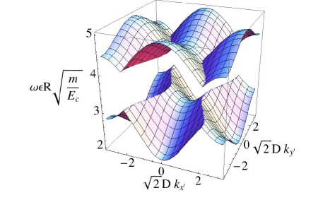
Figure 5: A plot of two of the eigenfrequencies of the AFE square lattice as a function of the in plane wave-vector, $\vec{k}^{\prime}$. The upper surface has been displaced upward by one unit for clarity. Without the displacement the two surfaces touch. The other two normal modes are equivalent to those plotted, but rotated by $\pi/2$. Note that all modes are gapped.

III.2 Quantum Phase Transition

It is not a priori obvious what will happen in the quantum mechanical case at zero temperature, since the quantum confinement introduces a new energy scale. Rather than solve for the variational groundstate of an $N\times N$ system directly, it was assumed that the quantum groundstate would possess the same symmetry as the classical system, so that only a $2\times 2$ unit cell of an (assumed) infinite system was analyzed. This has the advantage of following the correspondence principle as $\lambda\to\infty$. A plot of the variational energy for $\epsilon={1\over 2}$, reveals that at small values of the coupling constant, $\lambda$, a single minimum exists, Fig. (6). This minimum corresponds to $\beta=0$, i.e. a uniform distribution for the electronic wavefunction. As $\lambda$ increases past a critical value, two new minima emerge at $\beta=\pm{\pi\over 4}$ indicating a quantum phase transition. These values correspond to charge localizing normal to the plane. Furthermore, nearest neighbors polarize in opposite directions.

With the simple form of $\psi_{\rm var}$ of eq.(II.2) and the approximate interaction of eq.7, we can solve analytically for the minima of the variational energy and find:

$$\beta=\left\{\begin{array}[]{l l}{1\over 2}\arccos({192(22-{175\over\epsilon^{2}\lambda})\over 35(9\pi^{2}-512)})&\quad\mbox{if $\lambda\geq\lambda_{c}$;}\\ 0&\quad\mbox{if $\lambda<\lambda_{c}$.}\\ \end{array}\right.\$$ (15)

where $\alpha=\pi/2$ and $A=0$, and the critical value for the interaction is given by $\lambda_{c}={33600\over(22144-315\pi^{2})\epsilon^{2}}\approx 1.756/\epsilon^{2}$. Plotting $\beta$ for several values of $\epsilon$ reveals the phase transition, Fig. (7). Here, the analytical minimum result is confirmed numerically.

As $\epsilon$ shrinks, the transition becomes weaker, requiring the coupling constant, $\lambda$, to be large for the transition to occur. This phenomenon emerges from the geometry of the array. When the separation between shells becomes larger, the effective transition radius of each shell also increases, Fig. (8). The maximum value of $\epsilon$ can have is $1/2$, when the spheres touch. When $\epsilon$ is at its maximum there is a minimum $R$ below which quantum mechanics dominates and the system does not polarize: $R_{\rm min}\approx 7a_{0}m/m^{*}$. Thus we have the curious result that very small shells do not spontaneously polarize.

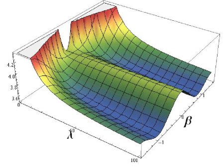
Figure 6: A plot of the energy functional from the quantum variational calculation for the 2D square lattice. Here, $\epsilon={1\over 2}$, thus the ratio of shell radius to separation is at a maximum (the close-packed condition). A single minimum for small values of the coupling constant, $\lambda$, occurs at $\beta=0$, where $\beta$ is the mixing parameter found in the variational wavefunction. This state corresponds with a uniform charge distribution. As $\lambda$ increases, two minima emerge at $\beta=\pm{\pi\over 4}$. These values correspond to charge localizing normal to the plane of the lattice.

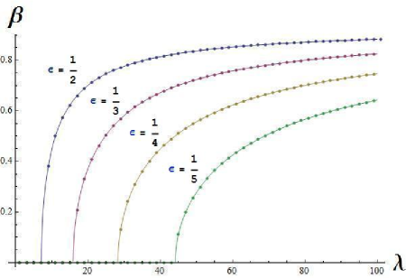
Figure 7: A plot of the quantum phase transition in the mixing parameter, $\beta$, of the variational wavefunction through the coupling constant, $\lambda$, for several values of $\epsilon$. This represents the system’s transition from uniform distribution to antiferroelectric order, through charge localization, Fig. (2). Analytical values of $\beta$ are given by Eq. 15. Here we see a good fit between numerical and analytical solutions.

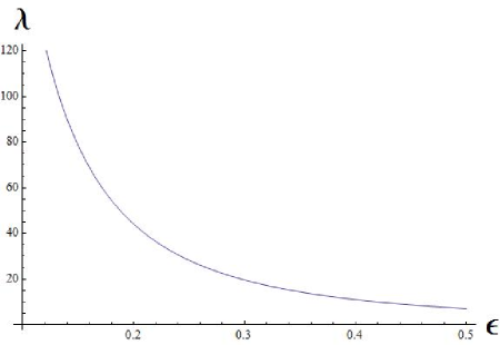
Figure 8: The critical value of the coupling constant $\lambda$, plotted against the ratio of shell radius to shell separation, $\epsilon$. It is at these values of $\lambda$ that the transition in the system occurs, given $\epsilon$. As separation increases, the coulomb interaction grows weaker, thus an even weaker confinement energy is required for the transition to occur. This corresponds with a larger physical radius for each shell, $\lambda\gg 1$.

IV 2D Triangular Lattice

Following our analysis of the 2D square lattice, we ues to the 2D triangular lattice. Experimental arrays made from the self-assembly of colloidal particles would likely stack in triangular arrays, rather than square ones.For the ring system the triangular lattice spontaneously breaks symmetry into a striped AFE phase with a six-fold degenerate groundstate. However, in that case the spins order in the plane, not perpendicular to it.

For a pure AFE Ising system the triangular lattice is frustrated.frustration While eq.(2) is not a simple Ising AFE interaction, it is clear that frustration will also be present. Monte Carlo simulation of eqn.(2 ) found multiple low energy states indicative of a glassy phase. There was no peak in the specific heat nor any abrupt change in the polarization to indicate an ordered phase. This meant there was no basis for a quantum mechanical ansatz to the ground state.

V 3D Face-Centered Cubic Lattice

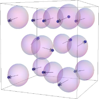
Figure 9: A typical low temperature state that anti-ferroelectric (AFE) in alternating horizontal planes. Each triangular lattice row has a common polarization in the plane, while neighboring rows have opposite polarization in the plane.

The next logical progression is to stack 2D triangular arrays forming a face-centered cubic (FCC) lattice. We chose this model since, in the close-packed limit, we expect it to be more physically reproducible through fabrication. Each lattice point has twelve nearest neighbors: four above, four in the plane, and four below. Again, the non-nearest neighbor interaction is considered negligible.

V.1 Classical Analysis

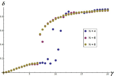
Figure 10: A plot of the classical phase transition from random alignment to the anti-ferroelectric (AFE) state Fig. (9) through $\gamma\equiv\beta E_{c}$, a measure of interaction strength, at zero temperature. Here $\delta$ is a measure of the system’s AFE order. Systems are face-centered cubic with periodic boundaries of size N=4, N=6, and N=8. Larger system sizes have sharper transitions.

Through numerical Monte Carlo simulation, a minimum energy was shown to exist when the system is in an AFE state by row. That is, each triangular lattice row of the FCC structure has opposite polarization, Fig. (9). Furthermore, a phase transition occurs from the unordered state to the AFE aligned state.

The temperature of the transition is determined by the interaction strength found in the Boltzmann factor, $\gamma\equiv\beta E_{c}=\beta e^{2}/D$, where $e$ is the charge of an electron, $\sqrt{2}D$ is the shell separation, and $\beta\equiv 1/kT$. One can see that with increased system size comes a sharper transition to the AFE state, Fig. (10). Numerical simulations indicated a persistent wobble about the in-plane polarization. Analytic expansion of the interaction about the uniform unpolarized state indicated an instability that pushes the polarization slightly off-axis. An expansion about the new minimum indicated restoring forces that were only quartic in the deviation from this state.

V.2 Quantum Mechanical Analysis

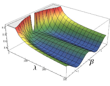
Figure 11: A plot of the energy functional from the quantum variational calculation for the 2D square lattice. Here, $\epsilon={1\over\sqrt{2}}$, thus the ratio of shell radius to separation is at a maximum (the close-packed condition). A single minimum for small values of the coupling constant, $\lambda$, occurs at $\beta=0$, where $\beta$ is the mixing parameter found in the variational wavefunction. This state corresponds with a uniform charge distribution. As $\lambda$ increases, two minima emerge at $\beta=\pm{\pi\over 4}$. These values correspond to charge localizing along the plane of the lattice.

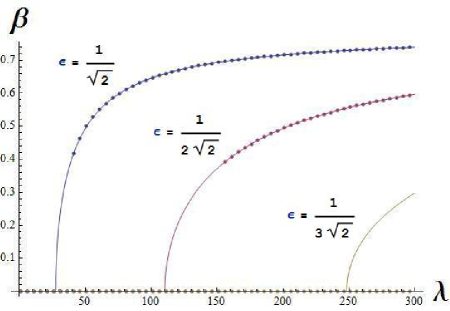
Figure 12: A plot of the quantum phase transition in the mixing parameter, $\beta$, of the variational wavefunction through the coupling constant, $\lambda$ for several values of $\epsilon$. This represents the system’s transition from uniform distribution to antiferroelectric order, through charge localization. Analytical values of $\beta$ are given by Eq. 18. Here we see a good fit between numerical and analytical solutions.

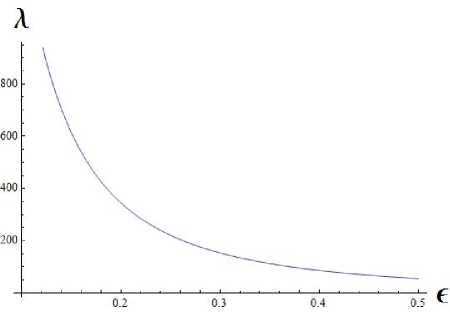
Figure 13: The critical value of the coupling constant $\lambda$, plotted against the ratio of shell radius to shell separation, $\epsilon$. It is at these values of $\lambda$ that the transition in the system occurs, given $\epsilon$. As separation increases, the coulomb interaction grows weaker, thus an even weaker confinement energy is required for the transition to occur. This corresponds with a larger physical radius for each shell, $\lambda\gg 1$.

To confirm our results from classical analysis, we turn to the Schrodinger variational principle as described earlier. We assumed that the low energy state in our quantum mechanical computations was polarized in the plane and alternated from one layer to the next, ignoring the slight wobble found in the classical analysis. (This will only give us an upper bound on the phase transition boundary). After completing the variational calculation, we once again find the charge to localize on each sphere to give the array an anti-ferroelectric alignment by triangular lattice row, Fig. (9). Furthermore, a quantum phase transition is found from uniform alignment to this state through the mixing parameter, $\beta$, found in the variational wavefunction, Fig. (12).

A plot of the energy functional under the close-packed condition, $\epsilon={1\over\sqrt{2}}$, reveals that at small values of the coupling constant, $\lambda$, a single minimum exists, Fig. (11). This minimum corresponds to $\beta=0$, i.e. a uniform distribution for the electronic wavefunction. As $\lambda$ increases past a critical value, two new minima emerge at $\beta=\pm\pi/4$. These values correspond with charge localizing along one of the axis of the shell. Furthermore, each triangular lattice row polarizes along opposite axes.

Analytically solving the energy functional for its minima, we find the ground state values of the variational parameters:

$$\beta=\left\{\begin{array}[]{l l}{1\over 2}\arccos({39\over\sqrt{2}\epsilon^{2}\lambda})&\quad\mbox{if $\lambda\geq\lambda_{c}$;}\\ 0&\quad\mbox{if $\lambda<\lambda_{c}$.}\\ \end{array}\right.\$$ (18)

and where $\alpha=\pi/2$ and $A=\pi/2$, where the critical value for the interaction is given by $\lambda_{c}={39\over\sqrt{2}\epsilon^{2}}$. Plotting $\beta$ for several values of $\epsilon$ reveals the aforementioned phase transition, Fig. (12). Here again, the analytical minimization result is confirmed numerically. As $\epsilon$ shrinks, the transition becomes weaker, requiring the coupling constant, $\lambda$, to be large for the transition to occur. This phenomenon emerges from the geometry of the array. When the separation between shells becomes larger, the effective transition radius of each shell also increases, Fig. (13).

It should be noted that this transition is weaker than that discovered for the 2D square lattice. Not only is the minimum coupling constant larger for each transition to occur, but also $\lambda_{c}$ increases at a quicker rate with increased separation, Fig. (13).

VI Conclusions

For a 2D square array and 3D FCC lattice of singly-charge quantum-dot quantum wells, a phase transition from the unordered state to a anti-ferroelectric state was found to occur at low energies through classical Monte Carlo simulation. Furthermore, this transition is confirmed through a quantum mechanical treatment of the system in which only nearest neighbor interactions are considered. The transition is a product of the geometry of the system, specifically dependent upon the ratio of shell radius to shell separation. Finally, this transition is said to be ”Ising-like,” which opens the doors to a host of known collective system behaviors.

For the square lattice we know that in order to have polarization, $\lambda>1.75/\epsilon^{2}$, which means that $R^{4}m^{*}/a_{0}D^{3},m>0.875$, where $a_{0}$ is the Bohr radius. For CdSe the effecive mass is $m^{*}/m=0.13$, a typical layer thickness is 0.43nm, and the capping (insulating) layer i about 1.6nm.pengdots If we assume that the shell is two monolayers thick, then we need shells with a radius of about 7nm in order to have a polarized ground state. If the shells have a smaller radius the kinetic cost to localize the electrons is too high. Charging the shells may prove to be too difficult at first; a simpler experiment would be to optically excite electron-hole pairs in a transverse electric field so as to create “chains” of elecron-holes across the core-shell array.

- (1) Paul Harrison, Quantum Wells, Wires and Dots : Theoretical and Computational Physics of Semiconductor Nanostructures. John Wiley & Sons, New York, 2005.
- (2) Jesse Berezovsky, Min Ouyang, Florian Meier, David D. Awschalom, David Battaglia and Xiaogang Peng, Phys. Rev. B 71, 081309 (2005).
- (3) Robert Pomraenke, Christoph Lienau, Yuriy I. Mazur, Zhiming M. Wang, Baolai Liang, Georgiy G. Tarasov, and Gregory J. Salamo, Phys. Rev. B 77, 075314 (2008).
- (4) JACS 129, 3339 (2007).
- (5) Dong Yu, Congjun Wang, Brian L. Wehrenberg, and Philippe Guyot-Sionnest, Phys. Rev. Lett. 92, 216802 (2004)
- (6) “A guide to Monte Carlo simulations in statistical physics ”, David Landau (Cambridge, UK ; New York : Cambridge University Press, 2005.)
- (7) Bahman Roostaei, Kieran J. Mullen, and A. T. Rezakhani, Polarization transitions in one-dimensional arrays of interacting rings, Phys. Rev. B 78, 075411 (2008).
- (8) Berezosky et al., Spin Dynamics and Level Structure of Quantum-Dot Quantum Wells. (cond-mat/0411181).
- (9) A. Lorke et al., Phys. Rev. Lett., 84, 2223 (2000).
- (10) Kerson Huang, “Statistical Mechanics”, (John Wiley and Sons, New York (1987)).
- (11) G. H. Wannier, Phys. Rev. 79, 357 - 364 (1950).