Intrinsic noise in stochastic models of gene expression with molecular memory and bursting

Abstract

Regulation of intrinsic noise in gene expression is essential for many cellular functions. Correspondingly, there is considerable interest in understanding how different molecular mechanisms of gene expression impact variations in protein levels across a population of cells. In this work, we analyze a stochastic model of bursty gene expression which considers general waiting-time distributions governing arrival and decay of proteins. By mapping the system to models analyzed in queueing theory, we derive analytical expressions for the noise in steady-state protein distributions. The derived results extend previous work by including the effects of arbitrary probability distributions representing the effects of molecular memory and bursting. The analytical expressions obtained provide insight into the role of transcriptional, post-transcriptional and post-translational mechanisms in controlling the noise in gene expression.

Regulation of gene expression is at the core of cellular adaptation and response to changing environments. Given that the underlying processes are intrinsically stochastic, cellular regulation must be designed to control variability (noise) in gene expression Kaern et al. (2005). While noise reduction is essential in many cases, regulatory mechanisms can also exploit the intrinsic stochasticity to increase noise and generate phenotypic heterogeneity in a clonal population of cells Raj and van Oudenaarden (2008). Quantifying the contributions of different sources of intrinsic noise using stochastic models of gene expression Paulsson (2005); Azaele et al. (2009); Munsky et al. (2009) is thus an important step towards understanding cellular processes and variations in cell populations.

Several recent studies have focused on quantifying noise in gene expression. Experiments have shown that protein production often occurs in ‘bursts’ Cai et al. (2006); Yu et al. (2006) and single-molecule measurements have also provided evidence for transcriptional bursting, i.e. production of mRNAs in bursts Golding et al. (2005); Raj et al. (2006); Chubb et al. (2006). The analysis and interpretation of such experimental studies has been aided by the development of coarse-grained stochastic models of gene expression. The simplest of these considers the basic processes (transcription, translation and degradation) as elementary Poisson processes Thattai and van Oudenaarden (2001) with exponential waiting-time distributions. However, since these processes are known to involve multiple biochemical steps, the corresponding waiting-time distributions can be more general than the ‘memoryless’ exponential distributionPedraza and Paulsson (2008). An important question then arises: how do gene expression mechanisms involving molecular memory effects influence the noise in protein distributions?

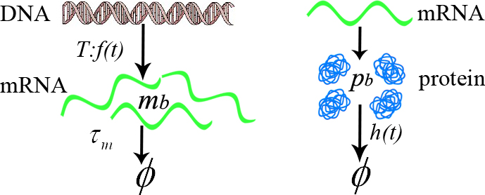
Figure 1: Reaction scheme for the underlying gene expression model. Production of mRNAs occurs in bursts (characterized by random variable $m_{b}$ with arbitrary distribution) and each mRNA gives rise to a burst of proteins (characterized by random variable $p_{b}$ with arbitrary distribution) before it decays (with lifetime $\tau_{m}$). The waiting-time distributions for burst arrival and decay of proteins are characterized by the functions $f(t)$ and $h(t)$ respectively.

Motivated by the preceding observations, we introduce a model including general waiting-time distributions for processes governing the arrival of bursts and the decay of proteins (termed ‘gestation’ and ‘senescence’ effects respectively Pedraza and Paulsson (2008)). The underlying reaction scheme for the models analyzed in this work is shown in Fig. 1. Production of mRNAs occurs in independent bursts and the time interval between the arrival of consecutive mRNA bursts is characterized by random variable $T$ with corresponding probability density function (p.d.f) $f(t)$. The number of mRNAs produced in a single transcriptional burst is characterized by the random variable $m_{b}$. Each mRNA independently gives rise to a random number of proteins (characterized by random variable $p_{b}$) before it is degraded. For the basic models of translation, $p_{b}$ follows the geometric distribution Cai et al. (2006); Yu et al. (2006); Friedman et al. (2006). However, more general schemes of gene expression (e.g. involving post-transcriptional regulation Jia and Kulkarni (2010)) can give rise to protein burst distributions that deviate significantly from a geometric distribution. Proteins are degraded independently and the waiting-time distribution for protein decay is characterized by the p.d.f $h(t)$.

In the limit that the mRNA lifetime ($\tau_{m}$) is much shorter than the protein lifetime ($\tau_{p}$), i.e. $\frac{\tau_{m}}{\tau_{p}}\ll 1$, the evolution of cellular protein concentrations can be modeled by processes governing arrival and decay of proteins alone Friedman et al. (2006); Shahrezaei and Swain (2008). Unless otherwise stated, the analysis in this paper will focus on this ‘burst’ limit, in which proteins are considered to arrive in independent instantaneous bursts arising from the underlying mRNA burst. In this limit, we have shown in recent work Elgart et al. (2010) that the processes involved in gene expression can be mapped on to models analyzed in queueing theory. In this mapping, individual proteins are the analogs of customers in queueing models. The bursty synthesis of proteins then corresponds to the arrival of customers in ‘batches’, whereas the protein decay-time distribution is the analog of the service-time distribution for each customer. Given that degradation of each protein is independent of others in the system, the process maps on to queueing systems with infinite servers. Correspondingly, the gene expression model in Fig. 1 maps on to what is known as a $GI^{X}/G/\infty$ system in the queueing literature. In this notation, the symbol $G$ refers to the general waiting-time distribution and $I^{X}$ indicates that the customers arrive in batches of random size $X$, where $X$ is drawn independently each time from an arbitrary distribution.

The $GI^{X}/G/\infty$ system has been analyzed in previous work in queueing theory Liu et al. (1990). In the following, we briefly review the notation and relevant results from the queueing theory analysis. As in Fig. 1, $f(t)$ and $h(t)$ denote the p.d.f. for the arrival time and service time respectively, with $F(t)$ and $H(t)$ as the corresponding cumulative density functions (c.d.f). The distribution of batch size $X$ has the corresponding generating function $A(z)$, defined as $A(z)=\sum_{i=1}^{\infty}{P(X=i)z^{i}}$. The $k$th factorial moment of batch size $X$, denoted by $A_{k}$, is given by $A_{k}=(d^{k}A(z)/dz^{k})|_{z=1}$. The number of customers in service at time $t$ is denoted by $N(t)$ and analytical expressions have been derived for the $r^{\mathrm{th}}$ binomial moment $B_{r}(t)$ of $N(t)$ Liu et al. (1990). These results can be used to derive expressions for all the moments of $N(t)$, for example $E[N(t)]=B_{1}(t)$ and $Var[N(t)]=2B_{2}(t)+B_{1}(t)-B_{1}^{2}(t)$. In the following, we will focus on two general subcategories of the $GI^{X}/G/\infty$ system for which closed-form analytical expressions can be derived for the mean and variance of steady-state protein distributions. These correspond to two cases: A) arbitrary distributions for gestation and bursting with a Poisson process governing protein degradation and B) arbitrary distributions for bursting and senescence with a Poisson process governing burst arrival.

Consider first case A, for which arbitrary gestation and bursting effects are included. In this case, the random variable $T$ characterizing the time interval between bursts is drawn from an arbitrary p.d.f. $f(t)$. The protein decay-time distribution $h(t)$ is taken to be an exponential function with $h(t)=\mu_{p}e^{-\mu_{p}t}$ and the mean protein lifetime is given by $\tau_{p}=1/\mu_{p}$. The corresponding queueing system is $GI^{X}/M/\infty$ where $M$ indicates that the process of customer departure, which is the analog of protein decay, is Markovian. $A(z)$ corresponds to the generating function of burst size distribution (determined by random variables $m_{b}$ and $p_{b}$ in Fig. 1) and $N(t)$ denotes the number of proteins in the cell at time $t$. The previous analysis Liu et al. (1990) has derived expressions for the steady-state mean and variance corresponding to $N=\lim_{t\to\infty}N(t)$ for the $GI^{X}/M/\infty$ queue as err :

$$E[N] = \frac{1}{\mu_{p}\langle T\rangle}A_{1}$$

$$Var[N] = E[N](1+\frac{f_{L}(\mu_{p})}{1-f_{L}(\mu_{p})}A_{1}-E[N]+\frac{A_{2}}{2A_{1}}),$$ (1)

where $\langle T\rangle$ is the mean of p.d.f $f(t)$ and $f_{L}(s)$ is the Laplace transform of $f(t)$.

To translate the result Eq.(1) into an expression for the noise in protein distributions, we derive expressions for $A_{1}$ and $A_{2}$ in terms of variables characterizing mRNA and protein burst distributions. In general, each mRNA will produce a random number of proteins ($p_{b}$) and furthermore the number of mRNAs in the burst is also a random variable ($m_{b}$). The number of proteins produced in a single burst is thus a compound random variable. Correspondingly, using standard results from probability theory Ross (2006), we derive the following equations for burst size parameters ($A_{1}$ and $A_{2}$) in terms of $m_{b}$ and $p_{b}$:

$$A_{1} = \langle m_{b}\rangle\langle p_{b}\rangle$$

$$A_{2} = \langle m_{b}\rangle(\sigma^{2}_{p_{b}}-\langle p_{b}\rangle)+(\sigma_{m_{b}}^{2}+\langle m_{b}\rangle^{2})\langle p_{b}\rangle^{2},$$ (2)

where the symbols $\langle..\rangle$ and $\sigma$ represent the mean and standard deviation respectively.

Using Eq.(2), in combination with identification of the random variable $N$ with the corresponding variable characterizing the number of proteins ($p_{s}$), we obtain the following expressions for the mean and coefficient of variance (noise) of the steady-state protein distribution:

$$\langle p_{s}\rangle = \frac{\tau_{p}}{\langle T\rangle}\langle m_{b}\rangle\langle p_{b}\rangle$$

$$\frac{\sigma^{2}_{p_{s}}}{\langle p_{s}\rangle^{2}} = \frac{1}{\langle p_{s}\rangle}+\frac{\langle T\rangle}{2\tau_{p}}\times\Bigl{(}K_{g}+\sigma^{2}_{m_{b}}/\langle m_{b}\rangle^{2}$$ (3)

$$+ \frac{\sigma^{2}_{p_{b}}/\langle p_{b}\rangle^{2}-1/\langle p_{b}\rangle}{\langle m_{b}\rangle}\Bigr{)},$$

where

$$K_{g}=2\Bigl{(}\frac{f_{L}(\mu_{p})}{1-f_{L}(\mu_{p})}-\frac{1}{\mu_{p}\langle T\rangle}\Bigr{)}+1,$$ (4)

is denoted as the gestation factor.

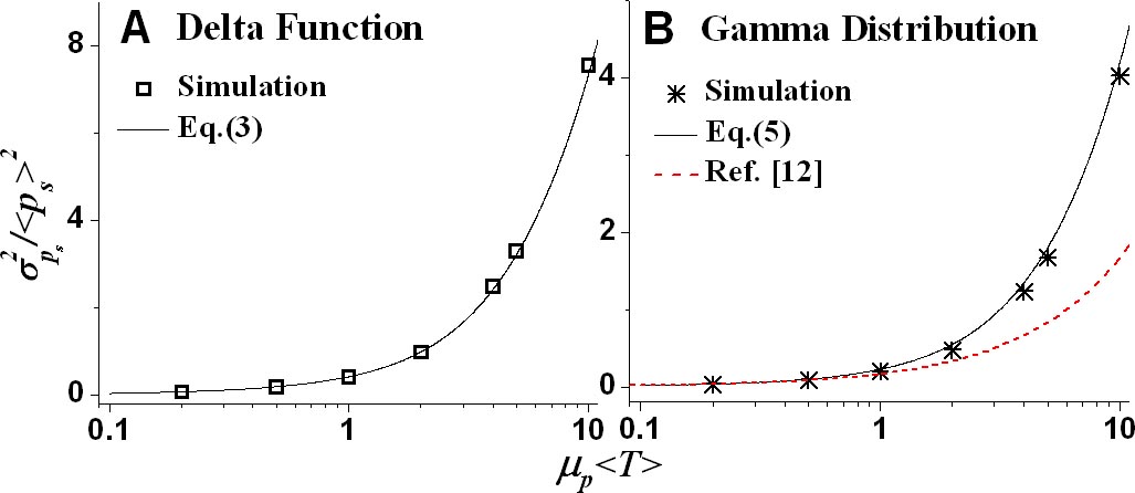
Figure 2: The noise vs $\mu_{p}\langle T\rangle$ from analytical expressions and stochastic simulations. A) The time interval between consecutive bursts is fixed and only 1 mRNA is produced each burst. The protein production is under post-transcriptional regulation Jia and Kulkarni (2010) such that $\sigma^{2}_{p_{b}}=0.67\langle p_{b}\rangle^{2}+\langle p_{b}\rangle$ and $\tau_{m}/\tau_{p}\approx 0.02$. B) The time interval between bursts is drawn from a Gamma distribution and the number of mRNAs created in one burst is drawn from a Poisson distribution. The number of proteins created by each mRNA follows a geometric distribution. The parameters are $\tau_{m}/\tau_{p}=0.2$, $\langle m_{b}\rangle=10$, $\sigma^{2}_{m_{b}}/\langle m_{b}\rangle^{2}=0.1$ and $\sigma^{2}_{T}/\langle T\rangle^{2}=0.2$. While Eq.(5) agrees with simulations, the result from Ref. Pedraza and Paulsson (2008) is less accurate when $\mu_{p}\langle T\rangle$ is large.

Different contributions to the noise in protein distributions are highlighted in Eq.(3): gestation effects, mRNA transcriptional bursting, and translational bursting from a single mRNA, which correspond to the terms $K_{g}$, $\sigma^{2}_{m_{b}}/\langle m_{b}\rangle^{2}$ and $\sigma^{2}_{p_{b}}/\langle p_{b}\rangle^{2}$, respectively. The first two terms can be modified by transcriptional regulation and the last term can be tuned by post-transcriptional regulation. It is noteworthy that each source contributes additively to the overall noise in the steady-state distribution. Moreover, while the noise due to gestation effects is independent of the degree of transcriptional bursting, the noise contribution from translational bursting is effectively reduced by transcriptional bursting.

While Eq.(3) is valid for general gestation effects, it is of interest to consider specific examples. We consider the case such that there is a constant delay between arrival of consecutive mRNA bursts, i.e. the waiting-time distribution is $f(t)=\delta(t-T_{d})$. In this case, the gestation factor is given by $K_{g}=2e^{-\mu_{p}T_{d}}/(1-e^{-\mu_{p}T_{d}})-2/\mu_{p}T_{d}+1$. The corresponding expression for the noise in protein distributions Eq.(3), considering a general case which also includes the effects of post-transcriptional regulation Jia and Kulkarni (2010), is in excellent agreement with results from stochastic simulations (Fig. 2A). It is noteworthy that $K_{g}$ can be nonvanishing even though the time interval between consecutive bursts is fixed (i.e. $\sigma^{2}_{T}=0$). In contrast to previous work Pedraza and Paulsson (2008), which suggests that the contribution of gestation effects to the noise vanishes when $\sigma^{2}_{T}=0$, our result shows that $K_{g}$ can be tuned from 0 to 1 as $\mu_{p}T_{d}$ is varied.

While the results derived above are valid in the limit $\tau_{m}\ll\tau_{p}$, an exact expression for the noise in the general case (i.e. without invoking the condition $\tau_{m}\ll\tau_{p}$ and for general gestation and bursting distributions) is difficult to obtain. However, a useful approximation can be obtained by noting that, for the basic gene expression models, the exact result is obtained by scaling the terms in the bracket in Eq.(3) with a time-averaging factor $\frac{\tau_{p}}{\tau_{m}+\tau_{p}}$ Paulsson (2005); Bar-Even et al. (2006). Using the approximation that the time-averaging factor is the same for general gestation and bursting distributions, we obtain

$$\frac{\sigma^{2}_{p_{s}}}{\langle p_{s}\rangle^{2}} \approx \frac{1}{\langle p_{s}\rangle}+\frac{\langle T\rangle}{2\tau_{p}}\times\Bigl{(}K_{g}+\sigma^{2}_{m_{b}}/\langle m_{b}\rangle^{2}$$ (5)

$$+ \frac{\sigma^{2}_{p_{b}}/\langle p_{b}\rangle^{2}-1/\langle p_{b}\rangle}{\langle m_{b}\rangle}\Bigr{)}\times\frac{\tau_{p}}{\tau_{m}+\tau_{p}},$$

It is instructive to compare Eq.(5) with the result derived in previous work Pedraza and Paulsson (2008) which assumes the basic protein production reaction scheme such that $\sigma^{2}_{p_{b}}=\langle p_{b}\rangle^{2}+\langle p_{b}\rangle$. Considering this specific case, we note that Eq.(5) is identical to the previous result Pedraza and Paulsson (2008) apart from the terms corresponding to the gestation factor $K_{g}$. The connection to the previous result can be seen by expanding the Laplace transform, $f_{L}(\mu_{p})$, in terms of moments of $T$. By assuming $\mu_{p}\langle T\rangle$ is small and $\langle T^{n}\rangle$ scales as the $n^{th}$ power of $\langle T\rangle$ or less, $K_{g}$ can be approximated by $K_{g}\approx\sigma^{2}_{T}/\langle T\rangle^{2}$ which corresponds to the previous result. Since the parameter $1/(\mu_{p}\langle T\rangle)$ measures the mean number of bursts occurring during the protein lifetime, this indicates that the previous result Pedraza and Paulsson (2008) is valid for the case of frequent bursting during a protein lifetime, and breaks down when bursts occur over larger time intervals (Fig. 2B).

We now consider case B, which corresponds to arbitrary distributions for bursting and senescence effects along with exponential waiting-time distributions for burst arrival. For this case, we take the waiting-time for protein degradation to be drawn from an arbitrary distribution characterized by p.d.f $h(t)$ and c.d.f $H(t)$. The waiting-time between consecutive bursts is characterized by an exponential distribution with $f(t)=\lambda e^{-\lambda t}$. The corresponding system, following the mapping to queueing theory, is the $M^{X}/G/\infty$ queue. The steady-state mean and variance of $N$ for this queue has been obtained in previous work Liu et al. (1990):

$$E[N] = \lambda A_{1}\int_{0}^{\infty}[1-H(t)]dt$$

$$Var[N] = E[N]+\lambda A_{2}\int_{0}^{\infty}[1-H(t)]^{2}dt.$$ (6)

By taking Eq.(2) and the relation $\langle T\rangle=1/\lambda$ into account, the mean and the noise for arbitrary senescence and bursting distribution can be derived as:

$$\langle p_{s}\rangle = \frac{A_{1}}{\langle T\rangle}\int_{0}^{\infty}[1-H(t)]dt=\frac{\tau_{p}}{\langle T\rangle}\langle m_{b}\rangle\langle p_{b}\rangle$$

$$\frac{\sigma^{2}_{p_{s}}}{\langle p_{s}\rangle^{2}} = \frac{1}{\langle p_{s}\rangle}+\frac{\langle T\rangle}{2\tau_{p}}\times\Bigl{(}1+\sigma^{2}_{m_{b}}/\langle m_{b}\rangle^{2}$$ (7)

$$+ \frac{\sigma^{2}_{p_{b}}/\langle p_{b}\rangle^{2}-1/\langle p_{b}\rangle}{\langle m_{b}\rangle}\Bigr{)}\times K_{s},$$

where

$$K_{s}=\frac{2\int_{0}^{\infty}[1-H(t)]^{2}dt}{\tau_{p}}=2-\frac{2\int_{0}^{\infty}H(t)[1-H(t)]dt}{\tau_{p}},$$ (8)

is denoted as the senescence factor.

It is noteworthy Eq.(7) and Eq.(3) have multiple terms in common. The terms characterizing the noise from transcriptional and translational bursting remain unchanged. However, unlike the gestation factor that contributes to the total noise additively, the senescence factor serves as a scaling factor for the total noise. While there is no obvious upper limit on the value of $K_{g}$, the upper bound for $K_{s}$ is 2 as is evident from Eq.(8). In general, as the distribution $h(t)$ grows more sharply peaked, the $K_{s}$ value increases. When $h(t)$ becomes a delta function, $K_{s}$ reaches its maximum value.

The general results derived in this work will serve as useful inputs for the analysis and interpretation of diverse experimental studies of gene expression. Some examples are: 1) Recent experiments on single-cell studies of HIV-1 viral infections have focused on the frequency and degree of transcriptional bursting Skupsky et al. (2010). For such studies, the derived results can be used to relate measurements of inter-arrival waiting-time distributions and burst distributions to the noise in protein distributions. 2) Experimental data and computational models of the cell-cycle in yeast indicate that modeling the basic processes of gene expression as Poisson processes gives rise to unrealistically large noise in protein distributions Kar et al. (2009), thereby suggesting that regulatory schemes which change distributions to reduce the noise are employed by the cell. The analytical expressions derived highlight different contributions to noise and can thus provide insight into how different regulatory schemes can lead to noise reduction. 3) More generally, the results derived can be used in the analysis of inverse problems, i.e. using experimental measurements of intrinsic noise to determine parameters of the underlying kinetic models. Such efforts, in turn, can lead to further insights into cellular factors that impact gene regulation, based on experimnetal observations of noise in gene expression.

In summary, we have analyzed the noise in protein distributions for general stochastic models of gene expression. The present work extends previous analysis by deriving analytical results for the noise in protein distributions for arbitrary gestation, senescence and bursting mechanisms. The expressions obtained provide insight into how different sources contribute to the noise in protein levels which can lead to phenotypic heterogeneity in isogenic populations. The results derived will thus serve as useful inputs for the analysis and interpretation of experiments probing stochastic gene expression and its phenotypic consequences. At a broader level, this work demonstrates the benefits of developing a mapping between models of stochastic gene expression and queueing systems which has potential applications for research in both fields. The extensive analytical approaches and tools developed in queueing theory can now be employed to analyze stochastic processes in gene expression. It is also anticipated that future analysis of regulatory mechanisms for gene expression will lead to new problems and challenges for queueing theory.

The authors acknowledge funding support from NSF (PHY-0957430) and from ICTAS, Virginia Tech.

References

- Kaern et al. (2005) M. Kaern, T. C. Elston, W. J. Blake, and J. J. Collins, Nat Rev Genet 6, 451 (2005).
- Raj and van Oudenaarden (2008) A. Raj and A. van Oudenaarden, Cell 135, 216 (2008).
- Paulsson (2005) J. M. Paulsson, Phys Of Life Rev 2, 157 (2005).
- Azaele et al. (2009) S. Azaele, J. R. Banavar, and A. Maritan, Phys. Rev. E 80 (2009).
- Munsky et al. (2009) B. Munsky, B. Trinh, and M. Khammash, Mol. Sys. Biol. 5 (2009).
- Cai et al. (2006) L. Cai, N. Friedman, and X. S. Xie, Nature 440, 358 (2006).
- Yu et al. (2006) J. Yu, J. Xiao, X. Ren, K. Lao, and X. S. Xie, Science 311, 1600 (2006).
- Golding et al. (2005) I. Golding, J. Paulsson, S. M. Zawilski, and E. C. Cox, Cell 123, 1025 (2005).
- Raj et al. (2006) A. Raj, C. S. Peskin, D. Tranchina, D. Y. Vargas, and S. Tyagi, PLoS Biol 4, e309 (2006).
- Chubb et al. (2006) J. Chubb, T. Trcek, S. Shenoy, and R. Singer, Curr. Biol. 16, 1018 (2006).
- Thattai and van Oudenaarden (2001) M. Thattai and A. van Oudenaarden, Proc Natl Acad Sci U S A 98, 8614 (2001).
- Pedraza and Paulsson (2008) J. M. Pedraza and J. Paulsson, Science 319, 339 (2008).
- Friedman et al. (2006) N. Friedman, L. Cai, and X. S. Xie, Phys Rev Lett 97, 168302 (2006).
- Jia and Kulkarni (2010) T. Jia and R. Kulkarni, Phys. Rev. Lett. 105, 018101 (2010).
- Shahrezaei and Swain (2008) V. Shahrezaei and P. S. Swain, Proc Natl Acad Sci USA 105, 17256 (2008).
- Elgart et al. (2010) V. Elgart, T. Jia, and R. V. Kulkarni, Phys. Rev. E 82, 021901 (2010).
- Liu et al. (1990) L. Liu, B. R. K. Kashyap, and J. G. C. Templeton, Jour. Appl. Prob. 27, 671 (1990).
- (18) The result given in Ref. [17] has a minor error which is corrected here.
- Ross (2006) S. M. Ross, Introduction to Probability Models, Ninth Edition (Academic Press, Inc., 2006).
- Bar-Even et al. (2006) A. Bar-Even, J. Paulsson, N. Maheshri, M. Carmi, E. O’Shea, Y. Pilpel, and N. Barkai, Nat Genet 38, 636 (2006).
- Skupsky et al. (2010) R. Skupsky, J. C. Burnett, J. E. Foley, D. V. Schaffer, and A. P. Arkin, PLoS Comput Biol 6, e1000952 (2010).
- Kar et al. (2009) S. Kar, W. T. Baumann, M. R. Paul, and J. J. Tyson, Proceedings of the National Academy of Sciences 106, 6471 (2009).