The power and Arnoldi methods in an algebra of circulants

Abstract

Circulant matrices play a central role in a recently proposed formulation of three-way data computations. In this setting, a three-way table corresponds to a matrix where each “scalar” is a vector of parameters defining a circulant. This interpretation provides many generalizations of results from matrix or vector-space algebra. We derive the power and Arnoldi methods in this algebra. In the course of our derivation, we define inner products, norms, and other notions. These extensions are straightforward in an algebraic sense, but the implications are dramatically different from the standard matrix case. For example, a matrix of circulants has a polynomial number of eigenvalues in its dimension; although, these can all be represented by a carefully chosen canonical set of eigenvalues and vectors. These results and algorithms are closely related to standard decoupling techniques on block-circulant matrices using the fast Fourier transform.

1 Introduction

We study iterative algorithms in a circulant algebra, which is a recent proposal for a set of operations that generalize matrix algebra to three-way data Kilmer et al. (2008). In particular, we extend this algebra with the ingredients required for iterative methods such as the power method and Arnoldi method, and study the behavior of these two algorithms.

Given an $m\times n\times k$ table of data, we view this data as an $m\times n$ matrix where each “scalar” is a vector of length $k$. We denote the space of length-$k$ scalars as $\mathbb{K}_{k}$. These scalars interact like circulant matrices. Circulant matrices are a commutative, closed class under the standard matrix operations. Indeed, $\mathbb{K}_{k}$ is the ring of circulant matrices, where we identify each circulant matrix with the $k$ parameters defining it.

Formally, let $\ushort{\alpha}\in\mathbb{K}_{k}$. Elements in the circulant algebra are denoted by an underline to distinguish them from regular scalars. When an element is written with an explicit parameter set, it is denoted by braces, for example

$$\ushort{\alpha}=\left\{\!\begin{smallmatrix}\alpha_{1}&\ldots&\alpha_{k}\end{smallmatrix}\!\right\}.$$

In what follows, we will use the notation $\leftrightarrow$ to provide an equivalent matrix-based notation for an operation involving $\mathbb{K}_{k}$. We define the operation $\operatorname{\texttt{circ}}(\cdot)$ as the “circulant matrix representation” of a scalar:

$$\ushort{\alpha}\quad\leftrightarrow\quad\operatorname{\texttt{circ}}(\ushort{\alpha})\equiv\begin{bmatrix}\alpha_{1}&\alpha_{k}&\ldots&\alpha_{2}\\ \alpha_{2}&\alpha_{1}&\ddots&\vdots\\ \vdots&\ddots&\ddots&\alpha_{k}\\ \alpha_{k}&\ldots&\alpha_{2}&\alpha_{1}\end{bmatrix}.$$ (1)

Let $\ushort{\alpha}$ be as above, and also let $\ushort{\beta}\in\mathbb{K}_{k}$. The basic addition and multiplication operations between scalars are then

$$\ushort{\alpha}+\ushort{\beta}\leftrightarrow\operatorname{\texttt{circ}}(\ushort{\alpha})+\operatorname{\texttt{circ}}(\ushort{\beta})\quad\text{ and }\quad\ushort{\alpha}\circ\ushort{\beta}\leftrightarrow\operatorname{\texttt{circ}}(\ushort{\alpha})\operatorname{\texttt{circ}}(\ushort{\beta}).$$ (2)

We use here a special symbol, the $\circ$ operation, to denote the product between these scalars, highlighting the difference from the standard matrix product. Note that the element

$$\ushort{1}=\left\{\!\begin{smallmatrix}1&0&\ldots&0\end{smallmatrix}\!\right\}$$

is the multiplicative identity.

Operations between vectors and matrices have similar, matricized, expressions. We use $\mathbb{K}_{k}^{n}$ to denote the space of length-$n$ vectors where each component is a $k$-vector in $\mathbb{K}_{k}$, and $\mathbb{K}_{k}^{m\times n}$ to denote the space of $m\times n$ matrices of these $k$-vectors. Thus, we identify each $m\times n\times k$ table with an element of $\mathbb{K}_{k}^{m\times n}$. Let $\ushort{\boldsymbol{A}}\in\mathbb{K}_{k}^{m\times n}$ and $\ushort{\mathbf{x}}\in\mathbb{K}_{k}^{n}$. Their product is:

$$\ushort{\boldsymbol{A}}\circ\ushort{\mathbf{x}}=\left[\begin{smallmatrix}\sum_{j=1}^{n}\ushort{A}_{1,j}\;\circ\;\ushort{x}_{j}\\ \vdots\\ \sum_{j=1}^{n}\ushort{A}_{m,j}\;\circ\;\ushort{x}_{j}\end{smallmatrix}\right]\leftrightarrow\left[\begin{smallmatrix}\operatorname{\texttt{circ}}(\ushort{A}_{1,1})&\ldots&\operatorname{\texttt{circ}}(\ushort{A}_{1,n})\\ \vdots&\ddots&\vdots\\ \operatorname{\texttt{circ}}(\ushort{A}_{m,1})&\ldots&\operatorname{\texttt{circ}}(\ushort{A}_{m,n})\end{smallmatrix}\right]\left[\begin{smallmatrix}\operatorname{\texttt{circ}}(\ushort{x}_{1})\\ \vdots\\ \operatorname{\texttt{circ}}(\ushort{x}_{n})\end{smallmatrix}\right].$$ (3)

Thus, we extend the operation $\operatorname{\texttt{circ}}$ to matrices and vectors of $\mathbb{K}_{k}$ scalars so that

$$\operatorname{\texttt{circ}}(\ushort{\boldsymbol{A}})\equiv\left[\begin{smallmatrix}\operatorname{\texttt{circ}}(\ushort{A}_{1,1})&\ldots&\operatorname{\texttt{circ}}(\ushort{A}_{1,n})\\ \vdots&\ddots&\vdots\\ \operatorname{\texttt{circ}}(\ushort{A}_{m,1})&\ldots&\operatorname{\texttt{circ}}(\ushort{A}_{m,n})\end{smallmatrix}\right]\quad\text{ and }\quad\operatorname{\texttt{circ}}(\ushort{\mathbf{x}})\equiv\left[\begin{smallmatrix}\operatorname{\texttt{circ}}(\ushort{x}_{1})\\ \vdots\\ \operatorname{\texttt{circ}}(\ushort{x}_{n})\end{smallmatrix}\right].$$ (4)

The definition of the product can now be compactly written as

$$\ushort{\boldsymbol{A}}\circ\ushort{\mathbf{x}}\leftrightarrow\operatorname{\texttt{circ}}(\ushort{\boldsymbol{A}})\operatorname{\texttt{circ}}(\ushort{\mathbf{x}}).$$ (5)

Of course this notation also holds for the special case of scalar-vector multiplication. Let $\ushort{\alpha}\in\mathbb{K}_{k}$. Then

$$\ushort{\mathbf{x}}\circ\ushort{\alpha}\leftrightarrow\operatorname{\texttt{circ}}(\ushort{\mathbf{x}})\operatorname{\texttt{circ}}(\ushort{\alpha}).$$

The above operations define the basic computational routines to treat $m\times n\times k$ arrays as $m\times n$ matrices of $\mathbb{K}_{k}$. They are equivalent to those proposed by Kilmer et al. (2008), and they constitute a module over vectors composed of circulants, as shown recently in Braman (To appear). Based on this analysis, we term the set of operations the circulant algebra. We note that these operations have more efficient implementations, which will be discussed in Sections 3 and 6.

The circulant algebra analyzed in this paper is closely related to the FIR matrix algebra due to Lambert (1996, Chapter 3). Lambert proposes an algebra of circulants; but his circulants are padded with additional zeros to better approximation a finite impulse response operator. He uses it to study blind deconvolution problems Lambert et al. (2001). As he observed, the relationship with matrices implies that many standard decompositions and techniques from real or complex valued matrix algebra carry over to the circulant algebra.

The circulant algebra in this manuscript is a particular instance of a matrix-over-a-ring, a long studied generalization of linear algebra Mcdonald (1984); Brewer et al. (1986). Prior work focuses on Roth theorems for the equation $AX-XB=C$ Gustafson (1979); generalized inverses Prasad (1994); completion and controllability problems Gurvits et al. (1992); matrices over the ring of integers for computer algebra systems Hafner and McCurley (1991); and transfer functions and linear dynamic systems Sontag (1976). Finally, see Gustafson (1991) for some interesting relationships between vectors space theory and module theory. A recent proposal extends many of the operations in Kilmer et al. (2008) to more general algebraic structures Navasca et al. (2010).

Let us provide some further context on related work. Multi-way arrays, tensors, and hypermatrices are a burgeoning area of research; see Kolda and Bader (2009) for a recent comprehensive survey. Some of the major themes are multi-linear operations, fitting multi-linear models, and multi-linear generalizations of eigenvalues Qi (2007). The formulation in this paper gives rise to stronger relationships with the literature on block-circulant matrices, which have been studied for quite some time. See Tee (2005) and the references therein for further historical and mathematical context on circulant matrices. In particular, Baker (1989) gives a procedure for the SVD of a block circulant that involves using the fast Fourier transform to decouple the problem into independent sub-problems, just as we shall do throughout this manuscript. Other work in this vein includes solving block-circulant systems that arise in the theory of antenna arrays: Sinnott and Harrington (1973); De Mazancourt and Gerlic (1983); Vescovo (1997).

The remainder of this paper is structured as follows. We first derive a few necessary operations in Section 2, including an inner product and norm. We then continue this discussion by studying these same operations using the Fourier transform of the underlying circulant matrices (Section 3). A few theoretical properties of eigenvalues in the circulant algebra are analyzed in Section 4. That section is a necessary prelude to the subsequent discussion of how the power method von Mises and Pollaczek-Geiringer (1929) and the Arnoldi method Krylov (1931); Lanczos (1950); Arnoldi (1951) generalize to this algebra, which comes in Section 5. We next explain how we implemented these operations in a Matlab package (Section 6); and we provide a numerical example of the algorithms (Section 7). Section 8 concludes the manuscript with some ideas for future work.

2 Operations with the power method

In the introduction, we provided the basic set of operations in the circulant algebra (eqs. (1)-(5)). We begin this section by stating the standard power method, and then follow by deriving the operations it requires.

Let $\boldsymbol{A}\in\mathbb{R}^{n\times n}$ and let $\mathbf{x}\in\mathbb{R}^{n}$ be an arbitrary starting vector. Then the power method proceeds by repeated applications of $\boldsymbol{A}$; see Figure 1 for a standard algorithmic description. (Line 6 checks for convergence and is one of several possible stopping criteria.) Under mild and well-known conditions (see Stewart (2001)), this iteration converges to the eigenvector with the largest magnitude eigenvalue.

Figure 1: The power method for a matrix $\boldsymbol{A}\in\mathbb{R}^{n\times n}$.

0:  $\boldsymbol{A},\mathbf{x}^{(0)},\tau$

1:  $\mathbf{x}^{(0)}\leftarrow\mathbf{x}^{(0)}\left\|\mathbf{x}^{(0)}\right\|^{-1}$

2:  for $k=1,\ldots,$ until convergence do

3:     $\mathbf{y}^{(k)}\leftarrow\boldsymbol{A}\mathbf{x}^{(k-1)}$

4:     $\alpha^{(k)}\leftarrow\left\|\mathbf{y}^{(k)}\right\|$

5:     $\mathbf{x}^{(k)}\leftarrow\mathbf{y}^{(k)}{\alpha^{(k)}}^{-1}$

6:     if ${\,\|{\operatorname{sign}(x_{1}^{(k)})\mathbf{x}^{(k)}-\operatorname{sign}(x_{1}^{(k-1)})\mathbf{x}^{(k-1)}}\|\,}<\tau$ then

7:        return  $\mathbf{x}^{(k)}$

8:     end if

9:  end for

Not all of the operations in Figure 1 are defined for the circulant algebra. In the first line, we use the norm $\left\|\mathbf{x}^{(0)}\right\|$ that returns a scalar in $\mathbb{R}$. We also use the scalar inverse $\alpha^{-1}$. The next operation is the $\operatorname{sign}$ function for a scalar. Let us define these operations, in order of their complexity. In the next section, we will reinterpret these operations in light of the relationships between the fast Fourier transform and circulant matrices. This will help illuminate a few additional properties of these operations and will let us state an ordering for elements.

2.1 The scalar inverse

We begin with the scalar inverse. Recall that all operations between scalars behave like circulant matrices. Thus, the inverse of $\ushort{\alpha}\in\mathbb{K}_{k}$ is

$$\ushort{\alpha}^{-1}\leftrightarrow\operatorname{\texttt{circ}}(\ushort{\alpha})^{-1}.$$

The matrix $\operatorname{\texttt{circ}}(\ushort{\alpha})^{-1}$ is also circulant Davis (1979).

2.2 Scalar functions and the angle function

Other scalar functions are also functions of a matrix (see Higham (2008)). Let $f$ be a function, then

$$f(\ushort{\alpha})\leftrightarrow f(\operatorname{\texttt{circ}}(\ushort{\alpha}))$$

where the right hand side is the same function applied to a matrix. (Note that it is not the function applied to the matrix element-wise.)

The sign function for a matrix is a special case. As explained in Higham (2008), the sign function applied to a complex value is the sign of the real-valued part. We wish to use a related concept that generalizes the real-valued sign that we term “angle.” Given a complex value $re^{\imath\theta}$, then $\operatorname{\texttt{angle}}(re^{\imath\theta})=e^{\imath\theta}$. For real or complex numbers $x$, we then have

$$\operatorname{\texttt{angle}}(x)\left|x\right|=x.$$

Thus, we define

$$\operatorname{\texttt{angle}}(\ushort{\alpha})\leftrightarrow\operatorname{\texttt{circ}}(\operatorname{\texttt{abs}}(\ushort{\alpha}))^{-1}\operatorname{\texttt{circ}}(\ushort{\alpha}).$$

2.3 Inner products, norms, and conjugates

We now proceed to define a norm. The norm of a vector in $\mathbb{K}_{k}^{n}$ produces a scalar in $\mathbb{K}_{k}$:

$$\left\|\ushort{\mathbf{x}}\right\|\leftrightarrow(\operatorname{\texttt{circ}}(\ushort{\mathbf{x}})^{*}\operatorname{\texttt{circ}}(\ushort{\mathbf{x}}))^{1/2}=\left(\sum_{i=1}^{n}\operatorname{\texttt{circ}}(\ushort{x}_{i})^{*}\operatorname{\texttt{circ}}(\ushort{x}_{i})\right)^{1/2}.$$

For a standard vector $\mathbf{x}\in\mathbb{C}^{n}$, the norm $\left\|\mathbf{x}\right\|=\sqrt{\mathbf{x}^{*}\mathbf{x}}$. This definition, in turn, follows from the standard inner product attached to the vector space $\mathbb{C}^{n}$. As we shall see, our definition has a similar interpretation. The inner product implied by our definition is

$$\langle{\ushort{\mathbf{x}}},{\ushort{\mathbf{y}}}\rangle\leftrightarrow\operatorname{\texttt{circ}}(\ushort{\mathbf{y}})^{*}\operatorname{\texttt{circ}}(\ushort{\mathbf{x}}).$$

Additionally, this definition implies that that the conjugate operation in the circulant algebra corresponds to the transpose of the circulant matrix

$$\overline{\ushort{\alpha}}\leftrightarrow\operatorname{\texttt{circ}}(\ushort{\alpha})^{*}.$$

With this conjugate, our inner product satisfies two of the standard properties: conjugate symmetry $\langle{\ushort{\mathbf{x}}},{\ushort{\mathbf{y}}}\rangle=\overline{\langle{\ushort{\mathbf{y}}},{\ushort{\mathbf{x}}}\rangle}$ and linearity $\langle{\ushort{\alpha}\circ\ushort{\mathbf{x}}},{\ushort{\mathbf{y}}}\rangle=\ushort{\alpha}\circ\langle{\ushort{\mathbf{x}}},{\ushort{\mathbf{y}}}\rangle$. The notion of positive definiteness is more intricate and we delay that discussion until after introducing a decoupling technique using the fast Fourier transform in the following section. Then, in Section 3.3, we use positive definiteness to demonstrate a Cauchy-Schwarz inequality, which in turn provides a triangle inequality for the norm.

3 Operations with the fast Fourier transform

In Section 2, we explained the basic operations of the circulant algebra as operations between matrices. All of these matrices consisted of circulant blocks. In this section, we show how to accelerate these operations by exploiting the relationship between the fast Fourier transform and circulant matrices.

Let $\boldsymbol{C}$ be a $k\times k$ circulant matrix. Then the eigenvector matrix of $\boldsymbol{C}$ is given by the $k\times k$ discrete Fourier transform matrix $\boldsymbol{F}$, where

$$F_{ij}=\frac{1}{\sqrt{k}}\omega^{(i-1)(j-1)}$$

and $\omega=e^{2\pi\imath/k}$. This matrix is complex symmetric, $\boldsymbol{F}^{T}=\boldsymbol{F}$, and unitary, $\boldsymbol{F}^{*}=\boldsymbol{F}^{-1}$. Thus, $\boldsymbol{C}=\boldsymbol{F}\boldsymbol{D}\boldsymbol{F}^{*}$, $\boldsymbol{D}=\operatorname{diag}(\lambda_{1},\ldots,\lambda_{k})$. Recall that multiplying a vector by $\boldsymbol{F}$ or $\boldsymbol{F}^{*}$ can be accomplished via the fast Fourier transform in $\mathcal{O}(k\log k)$ time instead of $\mathcal{O}(k^{2})$ for the typical matrix-vector product algorithm. Also, computing the matrix $\boldsymbol{D}$ can be done in time $O(k\log k)$ as well.

To express our operations, we define a new transformation, the “Circulant Fourier Transform” or $\operatorname{\texttt{cft}}$. Formally, $\operatorname{\texttt{cft}}:\ushort{\alpha}\in\mathbb{K}_{k}\mapsto\mathbb{C}^{k\times k}$ and its inverse $\operatorname{\texttt{icft}}:\mathbb{C}^{k\times k}\mapsto\mathbb{K}_{k}$ as follows:

$$\operatorname{\texttt{cft}}(\ushort{\alpha})\equiv\left[\begin{smallmatrix}\hat{\alpha}_{1}\\ &\ddots\\ &&\hat{\alpha}_{k}\end{smallmatrix}\right]=\boldsymbol{F}^{*}\operatorname{\texttt{circ}}(\ushort{\alpha})\boldsymbol{F},\qquad\operatorname{\texttt{icft}}\left(\left[\begin{smallmatrix}\hat{\alpha}_{1}\\ &\ddots\\ &&\hat{\alpha}_{k}\end{smallmatrix}\right]\right)\equiv\ushort{\alpha}\leftrightarrow\boldsymbol{F}\operatorname{\texttt{cft}}(\ushort{\alpha})\boldsymbol{F}^{*},$$

where $\hat{\alpha}_{j}$ are the eigenvalues of $\operatorname{\texttt{circ}}(\ushort{\alpha})$ as produced in the Fourier transform order. These transformations satisfy $\operatorname{\texttt{icft}}(\operatorname{\texttt{cft}}(\ushort{\alpha}))=\ushort{\alpha}$ and provide a convenient way of moving between operations in $\mathbb{K}_{k}$ to the more familiar environment of diagonal matrices in $\mathbb{C}^{k\times k}$.

The $\operatorname{\texttt{cft}}$ and $\operatorname{\texttt{icft}}$ transformations are extended to matrices and vectors over $\mathbb{K}_{k}$ differently than the $\operatorname{\texttt{circ}}$ operation we saw before. Observe that $\operatorname{\texttt{cft}}$ applied “element-wise” to the $\operatorname{\texttt{circ}}(\ushort{\boldsymbol{A}})$ matrix produces a matrix of diagonal blocks. In our extension of the $\operatorname{\texttt{cft}}$ routine, we perform an additional permutation to expose block-diagonal structure from these diagonal blocks. This permutation $\boldsymbol{P}_{m}\boldsymbol{A}\boldsymbol{P}_{n}^{T}$ transforms an $mk\times nk$ matrix of $k\times k$ diagonal blocks into a block diagonal $mk\times nk$ with $m\times n$ size blocks. It is also known as a stride permutation matrix Granata et al. (1992). The construction of $\boldsymbol{P}_{m}$, expressed in Matlab code is

p = reshape(1:m*k,k,m)’;
Pm = sparse(1:m*k,p(:),1,m*k,m*k);

The construction for $\boldsymbol{P}_{n}$ is identical. In Figure 2, we illustrate the overall transformation process that extends $\operatorname{\texttt{cft}}$ to matrices and vectors.

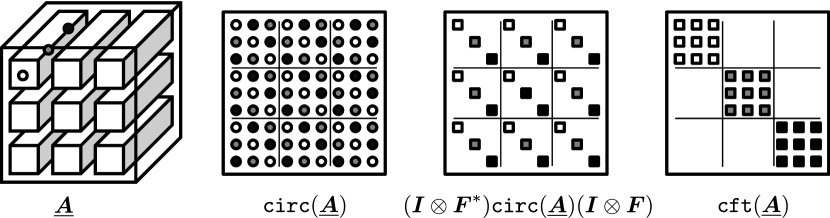
Figure 2: The sequence of transformations in our $\operatorname{\texttt{cft}}$ operation. Given a circulant $\boldsymbol{A}$, we convert it into a matrix by $\operatorname{\texttt{circ}}(\boldsymbol{A})$. The color of the circles in the figure is emphasizing the circulant structure, and not equality between blocks. In the third figure, we diagonalize each circulant using the Fourier transform. The pattern of eigenvalues is represented by squares. Here, we are coloring the squares to show the reordering induced by the permutation at the final step of the $\operatorname{\texttt{cft}}$ operation.

Algebraically, the $\operatorname{\texttt{cft}}$ operation for a matrix $\ushort{\boldsymbol{A}}\in\mathbb{K}_{k}^{m\times n}$ is

$$\operatorname{\texttt{cft}}(\ushort{\boldsymbol{A}})=\boldsymbol{P}_{m}(\boldsymbol{I}_{m}\otimes\boldsymbol{F}^{*})\operatorname{\texttt{circ}}(\ushort{\boldsymbol{A}})(\boldsymbol{I}_{n}\otimes\boldsymbol{F})\boldsymbol{P}_{n}^{T},$$

where $\boldsymbol{P}_{m}$ and $\boldsymbol{P}_{n}$ are the permutation matrices introduced above. We can equivalently write this directly in terms of the eigenvalues of each of the circulant blocks of $\operatorname{\texttt{circ}}(\ushort{\boldsymbol{A}})$:

$$\operatorname{\texttt{cft}}(\ushort{\boldsymbol{A}})\equiv\left[\begin{smallmatrix}\boldsymbol{\hat{A}}_{1}\\ &\ddots\\ &&\boldsymbol{\hat{A}}_{k}\end{smallmatrix}\right],\qquad\boldsymbol{\hat{A}}_{j}=\left[\begin{smallmatrix}\lambda_{j}^{1,1}&\ldots&\lambda_{j}^{1,n}\\ \vdots&\ddots&\vdots\\ \lambda_{j}^{m,1}&\ldots&\lambda_{j}^{m,n}\end{smallmatrix}\right],$$

where $\lambda_{1}^{r,s},\ldots,\lambda_{k}^{r,s}$ are the diagonal elements of $\operatorname{\texttt{cft}}(\ushort{A}_{r,s})$. The inverse operation $\operatorname{\texttt{icft}}$, takes a block diagonal matrix and returns the matrix in $\mathbb{K}_{k}^{m\times n}$:

$$\operatorname{\texttt{icft}}(\boldsymbol{A})\leftrightarrow(\boldsymbol{I}_{m}\otimes\boldsymbol{F})\boldsymbol{P}_{m}^{T}\boldsymbol{A}\boldsymbol{P}_{n}(\boldsymbol{I}_{n}\otimes\boldsymbol{F}^{*}).$$

Let us close this discussion by providing a concrete example of this operation.

Example 1.

Let $\ushort{\boldsymbol{A}}=\left[\begin{smallmatrix}\left\{\!\begin{smallmatrix}2&3&1\end{smallmatrix}\!\right\}&\left\{\!\begin{smallmatrix}8&\minus 2&0\end{smallmatrix}\!\right\}\\ \left\{\!\begin{smallmatrix}\minus 2&0&2\end{smallmatrix}\!\right\}&\left\{\!\begin{smallmatrix}3&1&1\end{smallmatrix}\!\right\}\end{smallmatrix}\right]$ . The result of the $\operatorname{\texttt{circ}}$ and $\operatorname{\texttt{cft}}$ operations, as illustrated in Figure 2, are:

$$\operatorname{\texttt{circ}}(\ushort{\boldsymbol{A}}) =\left[\begin{array}[]{>{\scriptstyle}c>{\scriptstyle}c>{\scriptstyle}c|>{\scriptstyle}c>{\scriptstyle}c>{\scriptstyle}c}2&1&3&8&0&\minus 2\\ 3&2&1&\minus 2&8&0\\ 1&3&2&0&\minus 2&8\\ \hline\cr\minus 2&2&0&3&1&1\\ 0&\minus 2&2&1&3&1\\ 2&0&\minus 2&1&1&3\end{array}\right],$$

$$(\boldsymbol{I}\otimes\boldsymbol{F}^{*})\operatorname{\texttt{circ}}(\ushort{\boldsymbol{A}})(\boldsymbol{I}\otimes\boldsymbol{F}) =\left[\begin{array}[]{>{\scriptstyle}c>{\scriptstyle}c>{\scriptstyle}c|>{\scriptstyle}c>{\scriptstyle}c>{\scriptstyle}c}6&\hfil&\hfil&6&\hfil&\hfil\\ \hfil&\minus\sqrt{3}\imath&\hfil&\hfil&\minus 9+\sqrt{3}\imath&\hfil\\ \hfil&\hfil&\sqrt{3}\imath&\hfil&\hfil&\minus 9-\sqrt{3}\imath\\ \hline\cr 0&\hfil&\hfil&5&\hfil&\hfil\\ \hfil&\minus 3+\sqrt{3}\imath&\hfil&\hfil&2&\hfil\\ \hfil&\hfil&\minus 3-\sqrt{3}\imath&\hfil&\hfil&2\\ \end{array}\right],$$

$$\operatorname{\texttt{cft}}(\ushort{\boldsymbol{A}}) =\left[\scriptstyle\begin{array}[]{>{\scriptstyle}c>{\scriptstyle}c|>{\scriptstyle}c>{\scriptstyle}c|>{\scriptstyle}c>{\scriptstyle}c}6&6&\hfil&\hfil&\hfil&\hfil\\ 0&5&\hfil&\hfil&\hfil&\hfil\\ \hline\cr\hfil&\hfil&\minus\sqrt{3}\imath&\minus 9+\sqrt{3}\imath\\ \hfil&\hfil&\minus 3+\sqrt{3}\imath&2\\ \hline\cr\hfil&\hfil&\hfil&\hfil&\sqrt{3}\imath&\minus 9-\sqrt{3}\imath\\ \hfil&\hfil&\hfil&\hfil&\minus 3-\sqrt{3}\imath&2\end{array}\right].$$

3.1 Operations

We now briefly illustrate how the $\operatorname{\texttt{cft}}$ accelerates and simplifies many operations. Let $\ushort{\alpha},\ushort{\beta}\in\mathbb{K}_{k}$. Note that

$$\ushort{\alpha}+\ushort{\beta} =\operatorname{\texttt{icft}}(\operatorname{\texttt{cft}}(\ushort{\alpha})+\operatorname{\texttt{cft}}(\ushort{\beta})),\text{ and }$$

$$\ushort{\alpha}\circ\ushort{\beta} =\operatorname{\texttt{icft}}(\operatorname{\texttt{cft}}(\ushort{\alpha})\operatorname{\texttt{cft}}(\ushort{\beta})).$$

In the Fourier space – the output of the $\operatorname{\texttt{cft}}$ operation – these operations are both $O(k)$ time because they occur between diagonal matrices. Due to the linearity of the $\operatorname{\texttt{cft}}$ operation, arbitrary sequences of operations in the Fourier space transform back seamlessly, for instance

$$\underbrace{(\ushort{\alpha}+\ushort{\beta})\circ(\ushort{\alpha}+\ushort{\beta})\circ\ldots\circ(\ushort{\alpha}+\ushort{\beta})}_{j\text{ times}}=\operatorname{\texttt{icft}}((\operatorname{\texttt{cft}}(\ushort{\alpha})+\operatorname{\texttt{cft}}(\ushort{\beta}))^{j}).$$

But even more importantly, these simplifications generalize to matrix-based operations too. For example,

$$\ushort{\boldsymbol{A}}\circ\ushort{\mathbf{x}}=\operatorname{\texttt{icft}}(\operatorname{\texttt{cft}}(\ushort{\boldsymbol{A}})\operatorname{\texttt{cft}}(\ushort{\mathbf{x}})).$$

In fact, in the Fourier space, this system is a series of independent matrix vector products:

$$\operatorname{\texttt{cft}}(\ushort{\boldsymbol{A}})\operatorname{\texttt{cft}}(\ushort{\mathbf{x}})=\left[\begin{smallmatrix}\boldsymbol{\hat{A}}_{1}\\ &\ddots\\ &&\boldsymbol{\hat{A}}_{k}\end{smallmatrix}\right]\left[\begin{smallmatrix}\mathbf{\hat{x}}_{1}\\ &\ddots\\ &&\mathbf{\hat{x}}_{k}\end{smallmatrix}\right]=\left[\begin{smallmatrix}\boldsymbol{\hat{A}}_{1}\mathbf{\hat{x}}_{1}\\ &\ddots\\ &&\boldsymbol{\hat{A}}_{k}\mathbf{\hat{x}}_{k}\end{smallmatrix}\right].$$

Here, we have again used $\boldsymbol{\hat{A}}_{j}$ and $\mathbf{\hat{x}}_{j}$ to denote the blocks of Fourier coefficients, or equivalently, circulant eigenvalues. The rest of the paper frequently uses this convention and shorthand where it is clear from context. This formulation takes

$$\underbrace{O(mnk\log k+nk\log k)}_{\operatorname{\texttt{cft}}\text{ and }\operatorname{\texttt{icft}}}+\underbrace{O(kmn)}_{\text{matvecs}}$$

operations instead of $O(mnk^{2})$ using the $\operatorname{\texttt{circ}}$ formulation in the previous section.

More operations are simplified in the Fourier space too. Let $\operatorname{\texttt{cft}}(\ushort{\alpha})=\operatorname{diag}\left[\begin{smallmatrix}\hat{\alpha}_{1},&\ldots,&\hat{\alpha}_{k}\end{smallmatrix}\right]$. Because the $\hat{\alpha}_{j}$ values are the eigenvalues of $\operatorname{\texttt{circ}}(\alpha)$, the following functions simplify:

$$\operatorname{\texttt{abs}}(\ushort{\alpha}) =\operatorname{\texttt{icft}}(\operatorname{diag}\left[\begin{smallmatrix}|\hat{\alpha}_{1}|,&\ldots,&|\hat{\alpha}_{k}|\end{smallmatrix}\right]),$$

$$\overline{\ushort{\alpha}} =\operatorname{\texttt{icft}}(\operatorname{diag}\left[\begin{smallmatrix}\overline{\hat{\alpha}_{1}},&\ldots,&\overline{\hat{\alpha}_{k}}\end{smallmatrix}\right])=\operatorname{\texttt{icft}}(\operatorname{\texttt{cft}}(\ushort{\alpha})^{*}),\text{ and }$$

$$\operatorname{\texttt{angle}}(\ushort{\alpha}) =\operatorname{\texttt{icft}}(\operatorname{diag}\left[\begin{smallmatrix}\hat{\alpha}_{1}/|\hat{\alpha}_{1}|,&\ldots,&\hat{\alpha}_{k}/|\hat{\alpha}_{k}|\end{smallmatrix}\right]).$$

Complex values in the CFT

A small concern with the $\operatorname{\texttt{icft}}$ operation is that it may produce complex-valued elements in $\mathbb{K}_{k}$. It suffices to note that when the output of a sequence of circulant operations produces a real-valued circulant, then the output of $\operatorname{\texttt{icft}}$ is also real-valued. In other words, there is no problem working in Fourier space instead of the real-valued circulant space. This fact can be formally verified by first formally stating the conditions under which $\operatorname{\texttt{icft}}$ produces real-valued circulants ($\operatorname{\texttt{icft}}(\boldsymbol{D})$ is real if and only if $\boldsymbol{F}^{2}\boldsymbol{D}\boldsymbol{F}^{2}=\boldsymbol{D}^{*}$, see Davis (1979)), and then checking that the operations in the Fourier space do not alter this condition.

3.2 Properties

Representations in Fourier space are convenient for illustrating some properties of these operations.

Proposition 2.

The matrix $\operatorname{\texttt{circ}}(\operatorname{\texttt{angle}}(\ushort{\alpha}))$ is orthogonal.

Proof.

We have

$$\operatorname{\texttt{circ}}(\operatorname{\texttt{angle}}(\ushort{\alpha}))^{*}\operatorname{\texttt{circ}}(\operatorname{\texttt{angle}}(\ushort{\alpha}))\leftrightarrow$$

$$\qquad\overline{\operatorname{\texttt{angle}}(\ushort{\alpha})}\circ\operatorname{\texttt{angle}}(\ushort{\alpha})=\operatorname{\texttt{icft}}\left(\left[\begin{smallmatrix}\overline{\hat{\alpha}}_{1}\hat{\alpha}_{1}/|\hat{\alpha}_{1}|^{2}\\ &\ddots\\ &&\overline{\hat{\alpha}}_{k}\hat{\alpha}_{k}/|\hat{\alpha}_{k}|^{2}\end{smallmatrix}\right]\right)=\ushort{1}.$$

∎

Additionally, the Fourier space is an easy place to understand spanning sets and bases in $\mathbb{K}_{k}^{m}$, as the following proposition shows.

Proposition 3.

Let $\ushort{\boldsymbol{X}}\in\mathbb{K}_{k}^{m\times n}$. Then $\ushort{\boldsymbol{X}}$ spans $\mathbb{K}_{k}^{m}$ if and only if $\operatorname{\texttt{circ}}(\ushort{\boldsymbol{X}})$ and $\operatorname{\texttt{cft}}(\ushort{\boldsymbol{X}})$ have rank $km$. Also $\ushort{\boldsymbol{X}}$ is a basis if and only if $\operatorname{\texttt{circ}}(\ushort{\boldsymbol{X}})$ and $\operatorname{\texttt{cft}}(\ushort{\boldsymbol{X}})$ are invertible.

Proof.

First note that $\operatorname{rank}(\operatorname{\texttt{cft}}(\ushort{\boldsymbol{X}}))=\operatorname{rank}(\operatorname{\texttt{circ}}(\ushort{\boldsymbol{X}}))$ because $\operatorname{\texttt{cft}}$ is a similarity transformation applied to $\operatorname{\texttt{circ}}$. It suffices to show this result for $\operatorname{\texttt{cft}}(\ushort{\boldsymbol{X}})$, then. Now consider $\ushort{\mathbf{y}}=\ushort{\boldsymbol{X}}\circ\ushort{\mathbf{a}}$:

$$\operatorname{\texttt{cft}}(\ushort{\mathbf{y}}) =\operatorname{\texttt{cft}}(\ushort{\boldsymbol{X}})\operatorname{\texttt{cft}}(\ushort{\mathbf{a}});$$

$$\left[\begin{smallmatrix}\mathbf{\hat{y}}_{1}\\ &\ddots\\ &&\mathbf{\hat{y}}_{k}\end{smallmatrix}\right] =\left[\begin{smallmatrix}\boldsymbol{\hat{X}}_{1}\\ &\ddots\\ &&\boldsymbol{\hat{X}}_{k}\end{smallmatrix}\right]\left[\begin{smallmatrix}\mathbf{\hat{a}}_{1}\\ &\ddots\\ &&\mathbf{\hat{a}}_{k}\end{smallmatrix}\right].$$

Thus, if there is a $\ushort{\mathbf{y}}$ that is feasible, then all $\boldsymbol{\hat{X}}_{j}\in\mathbb{C}^{m\times n}$ must be rank $m$. Conversely, if $\operatorname{\texttt{cft}}(\ushort{\boldsymbol{X}})$ has rank $km$ then each $\boldsymbol{\hat{X}}_{j}$ must have rank $m$, and any $\ushort{\mathbf{y}}$ is feasible. The result about the basis follows from an analogous argument. ∎

3.3 Inner products, norms, and ordering

We now return to our inner product and norm to elaborate on the positive-definiteness and the triangle inequality. In terms of the Fourier transform,

$$\langle{\ushort{\mathbf{x}}},{\ushort{\mathbf{y}}}\rangle=\operatorname{\texttt{icft}}(\operatorname{\texttt{cft}}(\ushort{\mathbf{y}})^{*}\operatorname{\texttt{cft}}(\ushort{\mathbf{x}})).$$

If we write this in terms of the blocks of Fourier coefficients then

$$\operatorname{\texttt{cft}}(\ushort{\mathbf{x}})^{*}\operatorname{\texttt{cft}}(\ushort{\mathbf{y}})=\left[\begin{smallmatrix}\mathbf{\hat{y}}_{1}^{*}\mathbf{\hat{x}}_{1}\\ &\ddots\\ &&\mathbf{\hat{y}}_{k}^{*}\mathbf{\hat{x}}_{k}\end{smallmatrix}\right].$$

For $\ushort{\mathbf{y}}=\ushort{\mathbf{x}}$, each diagonal term has the form $\mathbf{\hat{x}}_{j}^{*}\mathbf{\hat{x}}_{j}\geq 0$. Consequently, we do consider this a positive semi-definite inner product because the output $\operatorname{\texttt{circ}}(\langle{\ushort{\mathbf{x}}},{\ushort{\mathbf{y}}}\rangle)$ is a matrix with non-negative eigenvalues. This idea motivates the following definition of element ordering.

Definition 4 (Ordering).

Let $\ushort{\alpha},\ushort{\beta}\in\mathbb{K}_{k}$. We write

$$\ushort{\alpha}\leq\ushort{\beta}\qquad\text{ when } \qquad\operatorname{diag}(\operatorname{\texttt{cft}}(\ushort{\alpha}))\leq\operatorname{diag}(\operatorname{\texttt{cft}}(\ushort{\beta}))\quad\text{ element-wise, and}$$

$$\ushort{\alpha}<\ushort{\beta}\qquad\text{ when } \qquad\operatorname{diag}(\operatorname{\texttt{cft}}(\ushort{\alpha}))<\operatorname{diag}(\operatorname{\texttt{cft}}(\ushort{\beta}))\quad\text{ element-wise}.$$

We now show that our inner product satisfies the Cauchy-Schwarz inequality:

$$\operatorname{\texttt{abs}}{\langle{\ushort{\mathbf{x}}},{\ushort{\mathbf{y}}}\rangle}\leq\left\|\ushort{\mathbf{x}}\right\|\circ\left\|\ushort{\mathbf{y}}\right\|.$$

In Fourier space, this fact holds because $|\mathbf{\hat{y}}_{j}^{*}\mathbf{\hat{x}}_{j}|\leq\left\|\mathbf{\hat{x}}_{j}\right\|\left\|\mathbf{\hat{y}}_{j}\right\|$ follows from the standard Cauchy-Schwarz inequality. Using this inequality, we find that our norm satisfies the triangle inequality:

$$\left\|\ushort{\mathbf{x}}+\ushort{\mathbf{y}}\right\|^{2}=\langle{\ushort{\mathbf{x}}+\ushort{\mathbf{y}}},{\ushort{\mathbf{x}}+\ushort{\mathbf{y}}}\rangle\leq\langle{\ushort{\mathbf{x}}},{\ushort{\mathbf{x}}}\rangle+\ushort{2}\circ\left\|\ushort{\mathbf{x}}\right\|\circ\left\|\ushort{\mathbf{y}}\right\|+\langle{\ushort{\mathbf{y}}},{\ushort{\mathbf{y}}}\rangle=(\left\|\ushort{\mathbf{x}}\right\|+\left\|\ushort{\mathbf{y}}\right\|)^{2}.$$

In this expression, the constant $\ushort{2}$ is twice the multiplicative identify, that is $\ushort{2}=\left\{\!\begin{smallmatrix}2&0&\ldots&0\end{smallmatrix}\!\right\}$.

4 Eigenvalues and Eigenvectors

With the results of the previous few sections, we can now state and analyze an eigenvalue problem in circulant algebra. Braman (To appear) investigated these already and proposed a decomposition approach to compute them. We offer an extended analysis that addresses a few additional aspects. Specifically, we focus on a canonical set of eigenpairs.

Recall that eigenvalues of matrices are the roots of the characteristic polynomial $\det(\boldsymbol{A}-\lambda\boldsymbol{I})=0.$ Now let $\ushort{\boldsymbol{A}}\in\mathbb{K}_{k}^{n\times n}$ and $\ushort{\lambda}\in\mathbb{K}_{k}$. The eigenvalue problem does not change:

$$\det(\ushort{\boldsymbol{A}}-\ushort{\lambda}\circ\ushort{\boldsymbol{I}})=\ushort{0}.$$

(As an aside, note that the standard properties of the determinant hold for any matrix over a commutative ring with identity; in particular, the Cayley-Hamilton theorem holds in this algebra.) The existence of an eigenvalue implies the existence of a corresponding eigenvector $\ushort{\mathbf{x}}\in\mathbb{K}_{k}^{n}$. Thus, an eigenvalue and eigenvector pair in this algebra is

$$\ushort{\boldsymbol{A}}\circ\ushort{\mathbf{x}}=\ushort{\lambda}\circ\ushort{\mathbf{x}}.$$

Just like the matrix case, these eigenvectors can be rescaled by any constant $\ushort{\alpha}\in\mathbb{K}_{k}$: $\ushort{\boldsymbol{A}}\circ\ushort{\alpha}\circ\ushort{\mathbf{x}}=\ushort{\lambda}\circ\ushort{\alpha}\circ\ushort{\mathbf{x}}.$ In terms of normalization, note that $\left\|\ushort{\beta}\circ\ushort{\mathbf{x}}\right\|=\left\|\ushort{\mathbf{x}}\right\|$ if $\operatorname{\texttt{circ}}(\ushort{\beta})$ is an orthogonal circulant. This follows most easily by noting that

$$\left\|\ushort{\beta}\circ\ushort{\mathbf{x}}\right\|\leftrightarrow\left(\sum_{i=1}^{n}\operatorname{\texttt{circ}}(\ushort{\beta})^{*}\operatorname{\texttt{circ}}(\mathbf{x}_{i})^{*}\operatorname{\texttt{circ}}(\mathbf{x}_{i})\operatorname{\texttt{circ}}(\ushort{\beta})\right)^{1/2}\leftrightarrow\left\|\ushort{\mathbf{x}}\right\|,$$

because circulant matrices commute and $\operatorname{\texttt{circ}}(\ushort{\beta})$ is orthogonal by construction. For this reason, we consider orthogonal circulant matrices the analogues of angles or signs, and normalized eigenvectors in the circulant algebra can be rescaled by them. (Recall that we showed that $\operatorname{\texttt{angle}}(\ushort{\alpha})$ is an orthogonal circulant in Section 3.)

The Fourier transform offers a convenient decoupling procedure to compute eigenvalues and eigenvectors, as observed by Braman (To appear). Let $\ushort{\boldsymbol{A}}\in\mathbb{K}_{k}^{n\times n}$ and let $\ushort{\mathbf{x}}\in\mathbb{K}_{k}^{n}$ and $\ushort{\lambda}$ be an eigenvalue and eigenvector pair: $\ushort{\boldsymbol{A}}\circ\ushort{\mathbf{x}}=\ushort{\mathbf{x}}\circ\ushort{\lambda}$ and $\det(\ushort{\boldsymbol{A}}-\ushort{\lambda}\circ\ushort{\boldsymbol{I}})=0$. Then it is straightforward to show that the Fourier transforms $\operatorname{\texttt{cft}}(\ushort{\boldsymbol{A}})$, $\operatorname{\texttt{cft}}(\ushort{\mathbf{x}})$, and $\operatorname{\texttt{cft}}(\ushort{\lambda})$ decouple as follows:

$$\operatorname{\texttt{cft}}(\ushort{\boldsymbol{A}}\circ\ushort{\mathbf{x}}) =\operatorname{\texttt{cft}}(\ushort{\mathbf{x}}\circ\ushort{\lambda});$$

$$\operatorname{\texttt{cft}}(\ushort{\boldsymbol{A}})\operatorname{\texttt{cft}}(\ushort{\mathbf{x}}) =\operatorname{\texttt{cft}}(\ushort{\mathbf{x}})\operatorname{\texttt{cft}}(\ushort{\lambda});$$

$$\left[\begin{smallmatrix}\boldsymbol{\hat{A}}_{1}\\ &\ddots\\ &&\boldsymbol{\hat{A}}_{k}\end{smallmatrix}\right]\left[\begin{smallmatrix}\mathbf{\hat{x}}_{1}\\ &\ddots\\ &&\mathbf{\hat{x}}_{k}\end{smallmatrix}\right] =\left[\begin{smallmatrix}\mathbf{\hat{x}}_{1}\\ &\ddots\\ &&\mathbf{\hat{x}}_{k}\end{smallmatrix}\right]\left[\begin{smallmatrix}\hat{\lambda}_{1}\\ &\ddots\\ &&\hat{\lambda}_{k}\end{smallmatrix}\right];$$

$$\left[\begin{smallmatrix}\boldsymbol{\hat{A}}_{1}\mathbf{\hat{x}}_{1}\\ &\ddots\\ &&\boldsymbol{\hat{A}}_{k}\mathbf{\hat{x}}_{k}\end{smallmatrix}\right] =\left[\begin{smallmatrix}\hat{\lambda}_{1}\mathbf{\hat{x}}_{1}\\ &\ddots\\ &&\hat{\lambda}_{k}\mathbf{\hat{x}}_{k}\end{smallmatrix}\right],$$

where $\hat{\lambda}_{j}\in\lambda(\boldsymbol{\hat{A}}_{j})$ and $\mathbf{\hat{x}}_{j}\not=0$. The last equation follows because

$$\operatorname{\texttt{cft}}(\det(\ushort{\boldsymbol{A}}-\ushort{\lambda}\circ\ushort{I}))=\operatorname{diag}\left[\begin{smallmatrix}\det(\boldsymbol{\hat{A}}_{1}-\hat{\lambda}_{1}\boldsymbol{I}),&\ldots,&\det(\boldsymbol{\hat{A}}_{k}-\hat{\lambda}_{k}\boldsymbol{I})\end{smallmatrix}\right]=0.$$

The decoupling procedure we just described shows that any eigenvalue or eigenvector of $\ushort{\boldsymbol{A}}$ must decompose into individual eigenvalues or eigenvectors of the $\operatorname{\texttt{cft}}$-transformed problem. This illustrates a fundamental difference from the standard matrix algebra. For standard matrices, requiring $\det(\boldsymbol{A}-\lambda\boldsymbol{I})=0$ and finding a nonzero solution $\mathbf{x}$ for $\boldsymbol{A}\mathbf{x}=\lambda\mathbf{x}$ are equivalent. In contrast, the determinant and the eigenvector equations are not equivalent in the circulant algebra: $\ushort{\boldsymbol{A}}\circ\ushort{\mathbf{x}}=\ushort{\mathbf{x}}\circ\ushort{\lambda}$ actually has an infinite number of solutions $\ushort{\lambda}$. For instance, set $\mathbf{\hat{x}}_{1},\hat{\lambda}_{1}$ to be an eigenpair of $\boldsymbol{\hat{A}}_{1}$ and $\mathbf{\hat{x}}_{j}=0$ for $j>1$, then any value for $\hat{\lambda}_{j}$ solves $\ushort{\boldsymbol{A}}\circ\ushort{\mathbf{x}}=\ushort{\mathbf{x}}\circ\ushort{\lambda}$. However, only a few of these solutions also satisfy $\det(\ushort{\boldsymbol{A}}-\ushort{\lambda}\circ\ushort{\boldsymbol{I}})=\ushort{0}$.

Eigenvalues of matrices in $\mathbb{K}_{k}^{n\times n}$ have some interesting properties. Most notably, a matrix may have more than $n$ eigenvalues. As a special case, the diagonal elements of a matrix are not necessarily the only eigenvalues. We demonstrate these properties with an example.

Example 5.

For the diagonal matrix

$$\begin{bmatrix}\left\{\!\begin{smallmatrix}2&3&1\end{smallmatrix}\!\right\}&\left\{\!\begin{smallmatrix}0&0&0\end{smallmatrix}\!\right\}\\ \left\{\!\begin{smallmatrix}0&0&0\end{smallmatrix}\!\right\}&\left\{\!\begin{smallmatrix}3&1&1\end{smallmatrix}\!\right\}\end{bmatrix}$$

we have

$$\boldsymbol{\hat{A}}_{1}=\begin{bmatrix}6&0\\ 0&5\end{bmatrix},\quad\boldsymbol{\hat{A}}_{2}=\begin{bmatrix}\minus\imath\sqrt{3}&0\\ 0&2\end{bmatrix},\quad\boldsymbol{\hat{A}}_{3}=\begin{bmatrix}\imath\sqrt{3}&0\\ 0&2\end{bmatrix}.$$

Thus,

$$\ushort{\lambda}_{1} =\operatorname{\texttt{icft}}(\operatorname{diag}\left[\begin{smallmatrix}6&2&2\end{smallmatrix}\right])=\begin{smallmatrix}(1/3)\end{smallmatrix}\left\{\!\begin{smallmatrix}10&4&4\end{smallmatrix}\!\right\} \qquad\ushort{\lambda}_{2} =\operatorname{\texttt{icft}}(\operatorname{diag}\left[\begin{smallmatrix}5&\minus\imath\sqrt{3}&\imath\sqrt{3}\end{smallmatrix}\right])=\begin{smallmatrix}(1/3)\end{smallmatrix}\left\{\!\begin{smallmatrix}5&2&2\end{smallmatrix}\!\right\}$$

$$\ushort{\lambda}_{3} =\operatorname{\texttt{icft}}(\operatorname{diag}\left[\begin{smallmatrix}6&\minus\imath\sqrt{3}&\imath\sqrt{3}\end{smallmatrix}\right])=\left\{\!\begin{smallmatrix}2&3&1\end{smallmatrix}\!\right\} \qquad\ushort{\lambda}_{4} =\operatorname{\texttt{icft}}(\operatorname{diag}\left[\begin{smallmatrix}5&2&2\end{smallmatrix}\right])=\begin{smallmatrix}(1/3)\end{smallmatrix}\left\{\!\begin{smallmatrix}3&1&1\end{smallmatrix}\!\right\}.$$

The corresponding eigenvectors are

$$\begin{array}[]{l@{\qquad}l}\ushort{\mathbf{x}}_{1}=\begin{bmatrix}\left\{\!\begin{smallmatrix}1/3&1/3&1/3\end{smallmatrix}\!\right\}\\ \left\{\!\begin{smallmatrix}2/3&\minus 1/3&\minus 1/3\end{smallmatrix}\!\right\}\end{bmatrix};&\ushort{\mathbf{x}}_{2}=\begin{bmatrix}\left\{\!\begin{smallmatrix}2/3&\minus 1/3&\minus 1/3\end{smallmatrix}\!\right\}\\ \left\{\!\begin{smallmatrix}1/3&1/3&1/3\end{smallmatrix}\!\right\}\end{bmatrix};\\[12.91663pt] \ushort{\mathbf{x}}_{3}=\begin{bmatrix}\left\{\!\begin{smallmatrix}1&0&0\end{smallmatrix}\!\right\}\\ \left\{\!\begin{smallmatrix}0&0&0\end{smallmatrix}\!\right\}\end{bmatrix};&\ushort{\mathbf{x}}_{4}=\begin{bmatrix}\left\{\!\begin{smallmatrix}0&0&0\end{smallmatrix}\!\right\}\\ \left\{\!\begin{smallmatrix}1&0&0\end{smallmatrix}\!\right\}\end{bmatrix}.\end{array}$$

There are still more eigenvalues, however. The four eigenvalues above all correspond to elements in $\mathbb{K}_{k}$ with real-valued entries. We can combine the eigenvalues of the $\boldsymbol{\hat{A}}_{j}$’s to produce complex-valued elements in $\mathbb{K}_{k}$ that are also eigenvalues. These are

$$\ushort{\lambda}_{5} =\operatorname{\texttt{icft}}(\operatorname{diag}\left[\begin{smallmatrix}6&\minus\imath\sqrt{3}&2\end{smallmatrix}\right]) \qquad\ushort{\lambda}_{6} =\operatorname{\texttt{icft}}(\operatorname{diag}\left[\begin{smallmatrix}6&2&\imath\sqrt{3}\end{smallmatrix}\right])$$

$$\ushort{\lambda}_{7} =\operatorname{\texttt{icft}}(\operatorname{diag}\left[\begin{smallmatrix}5&\minus\imath\sqrt{3}&2\end{smallmatrix}\right]) \qquad\ushort{\lambda}_{8} =\operatorname{\texttt{icft}}(\operatorname{diag}\left[\begin{smallmatrix}5&2&\imath\sqrt{3}\end{smallmatrix}\right]).$$

For completeness and further clarity, let us extend this example a bit by presenting also the eigenvalues of the non-diagonal matrix from Example 1. Let $\ushort{\boldsymbol{A}}=\left[\begin{smallmatrix}\left\{\!\begin{smallmatrix}2&3&1\end{smallmatrix}\!\right\}&\left\{\!\begin{smallmatrix}8&\minus 2&0\end{smallmatrix}\!\right\}\\ \left\{\!\begin{smallmatrix}\minus 2&0&2\end{smallmatrix}\!\right\}&\left\{\!\begin{smallmatrix}3&1&1\end{smallmatrix}\!\right\}\end{smallmatrix}\right]$ . The $\operatorname{\texttt{cft}}$ produces:

$$\boldsymbol{\hat{A}}_{1}=\begin{bmatrix}6&6\\ 0&5\end{bmatrix},\quad\boldsymbol{\hat{A}}_{2}=\begin{bmatrix}\minus\sqrt{3}&\minus 9+\imath\sqrt{3}\\ \minus 3+\imath\sqrt{3}&2\end{bmatrix},\quad\boldsymbol{\hat{A}}_{3}=\begin{bmatrix}\imath\sqrt{3}&\minus 9-\imath\sqrt{3}\\ \minus 3+\imath\sqrt{3}&2\end{bmatrix}.$$

The numerical eigenvalues of $\boldsymbol{\hat{A}}_{1}$ are $\{6,5\}$; of $\boldsymbol{\hat{A}}_{2}$ are $\{\minus 0.0899+6.4282\imath,2.0899-4.6962\imath\}$; and of $\boldsymbol{\hat{A}}_{3}$ are $\{\minus 0.0899-6.4282\imath,2.0899+4.6962\imath\}$. The real-valued eigenvalues of $\ushort{\boldsymbol{A}}$ are

$$\ushort{\lambda}_{1} =\left\{\!\begin{smallmatrix}1.9401&\minus 1.6814&5.7413\end{smallmatrix}\!\right\} \ushort{\lambda}_{2} =\left\{\!\begin{smallmatrix}3.0599&3.6814&\minus 1.7413\end{smallmatrix}\!\right\}$$

$$\ushort{\lambda}_{3} =\left\{\!\begin{smallmatrix}3.3933&4.0147&\minus 1.4080\end{smallmatrix}\!\right\} \ushort{\lambda}_{4} =\left\{\!\begin{smallmatrix}1.6067&\minus 2.0147&5.4080\end{smallmatrix}\!\right\}.$$

The complex-valued eigenvalues of $\ushort{\boldsymbol{A}}$ are

$$\ushort{\lambda}_{5} =\left\{\!\begin{smallmatrix}4.6966-1.5654\imath,&\minus 0.7040+1.9114\imath,&2.0073-0.3461\imath\end{smallmatrix}\!\right\}$$

$$\ushort{\lambda}_{6} =\left\{\!\begin{smallmatrix}3.6367+2.1427\imath,&3.0373+0.3980\imath,&\minus 0.6740-2.5407\imath\end{smallmatrix}\!\right\}$$

$$\ushort{\lambda}_{7} =\left\{\!\begin{smallmatrix}4.3633-1.5654\imath,&\minus 1.0373+1.9114\imath,&1.6740-0.3461\imath\end{smallmatrix}\!\right\}$$

$$\ushort{\lambda}_{8} =\left\{\!\begin{smallmatrix}3.3034+2.1427\imath,&2.7040+0.3980\imath,&\minus 1.0073-2.5407\imath\end{smallmatrix}\!\right\}.$$

We now count the number of unique eigenvalues and eigenvectors, using the decoupling procedure in the Fourier space. To simplify the discussion, let us only consider the case where each $\boldsymbol{\hat{A}}_{j}$ has simple eigenvalues. Consider an $\ushort{\boldsymbol{A}}\in\mathbb{K}_{k}^{n\times n}$ with this property, and let $m_{j}$ be the number of unique eigenvalues and eigenvectors of $\boldsymbol{\hat{A}}_{j}$. Then the number of unique eigenvalues of $\ushort{\boldsymbol{A}}$ is given by the number of unique solutions to $\det(\ushort{\boldsymbol{A}}-\ushort{\lambda}\circ\ushort{\boldsymbol{I}})=0$ which is $\prod_{j=1}^{k}m_{j}$. The number of unique eigenvectors (up to normalization) is given by the number of unique solutions to $\ushort{\boldsymbol{A}}\circ\ushort{\mathbf{x}}=\ushort{\mathbf{x}}\circ\ushort{\lambda}$, which is also $\prod_{j=1}^{k}m_{j}$.

This result shows there are at most $n^{k}$ eigenvalues if $\ushort{\lambda}\in\mathbb{K}_{k}$ is allowed to be complex-valued, even when $\ushort{\boldsymbol{A}}\in\mathbb{K}_{k}$ is real-valued. If $\ushort{\boldsymbol{A}}\in\mathbb{K}_{k}$ is real-valued, then there are at most $n^{\lceil(k+1)/2\rceil}$ “real” eigenvalues. For this result, note that $\operatorname{\texttt{icft}}(\operatorname{diag}\left[\begin{smallmatrix}\alpha_{1}&\ldots&\alpha_{k}\end{smallmatrix}\right])$ is real-valued if and only if $\operatorname{diag}\left[\begin{smallmatrix}\alpha_{1}&\ldots&\alpha_{k}\end{smallmatrix}\right]^{*}=\boldsymbol{F}^{2}\operatorname{diag}\left[\begin{smallmatrix}\alpha_{1}&\ldots&\alpha_{k}\end{smallmatrix}\right]\boldsymbol{F}^{2}$ Davis (1979), where $\boldsymbol{F}$ is the Fourier transform matrix. This implies $\alpha_{1}$ is real-valued, and $\alpha_{j}=\overline{\alpha_{k-j+1}}$. Applying this restriction reduces the feasible combinations of eigenvalues to $n^{\lceil(k+1)/2\rceil}$.

Given that there are so many eigenvalues and vectors, are all of them necessary to describe $\ushort{\boldsymbol{A}}$? We now show this is not the case by making a few definitions to clarify the discussion.

Definition 6.

Let $\ushort{\boldsymbol{A}}\in\mathbb{K}_{k}^{n\times n}$. A canonical set of eigenvalues and eigenvectors is a set of minimum size, ordered such that $\operatorname{\texttt{abs}}(\ushort{\lambda}_{1})\geq\operatorname{\texttt{abs}}(\ushort{\lambda}_{2})\geq\ldots\geq\operatorname{\texttt{abs}}(\ushort{\lambda}_{k})$, which contains the information to reproduce any eigenvalue or eigenvector of $\ushort{\boldsymbol{A}}$

In the diagonal matrix from Example 5, the sets $\{(\ushort{\lambda}_{1},\ushort{\mathbf{x}}_{1}),(\ushort{\lambda}_{2},\ushort{\mathbf{x}}_{2})\},$ $\{(\ushort{\lambda}_{3},\ushort{\mathbf{x}}_{3}),(\ushort{\lambda}_{4},\ushort{\mathbf{x}}_{4})\},$ and $\{(\ushort{\lambda}_{1},\ushort{\mathbf{x}}_{1}),(\ushort{\lambda}_{3},\ushort{\mathbf{x}}_{3}),(\ushort{\lambda}_{4},\ushort{\mathbf{x}}_{4})\}$ contain all the information to reproduce any eigenpair, whereas the set $\{(\ushort{\lambda}_{1},\ushort{\mathbf{x}}_{1}),(\ushort{\lambda}_{3},\ushort{\mathbf{x}}_{3})\}$ does not (it does not contain the eigenvalue $5$ of $\boldsymbol{\hat{A}}_{1}$). In this case, the only canonical set is $\{(\ushort{\lambda}_{1},\ushort{\mathbf{x}}_{1}),(\ushort{\lambda}_{2},\ushort{\mathbf{x}}_{2})\}$. This occurs because, by a simple counting argument, a canonical set must have at least two eigenvalues, thus the set is of minimum size. The choice of $\ushort{\lambda}_{1}$ and $\ushort{\lambda}_{2}$ is given by the ordering condition. Among all the size $2$ sets with all the information, this is the only one with the property that $\operatorname{\texttt{abs}}(\ushort{\lambda}_{1})\geq\operatorname{\texttt{abs}}(\ushort{\lambda}_{2})$.

Theorem 7 (Unique Canonical Decomposition).

Let $\ushort{\boldsymbol{A}}\in\mathbb{K}_{k}^{n\times n}$ where each $\boldsymbol{\hat{A}}_{j}$ in the $\operatorname{\texttt{cft}}(\ushort{\boldsymbol{A}})$ matrix has distinct eigenvalues with distinct magnitudes. Then $\ushort{\boldsymbol{A}}$ has a unique canonical set of $n$ eigenvalues and eigenvectors. This canonical set corresponds to a basis of $n$ eigenvectors, yielding an eigendecomposition

$$\ushort{\boldsymbol{A}}=\ushort{\boldsymbol{X}}\circ\ushort{\boldsymbol{\Lambda}}\circ\ushort{\boldsymbol{X}}^{-1}.$$

Proof.

Because all of the eigenvalues of each $\boldsymbol{\hat{A}}_{j}$ are distinct, with distinct magnitudes, there are $nk$ distinct numbers. This implies that any canonical set must have at least $n$ eigenvalues.

Let $\hat{\lambda}_{j}^{(i)}$ be the $i$th eigenvalue of $\boldsymbol{\hat{A}}_{j}$ ordered such that $|\hat{\lambda}_{j}^{(1)}|>|\hat{\lambda}_{j}^{(2)}|>\ldots>|\hat{\lambda}_{j}^{(n)}|$. Then $\ushort{\lambda}_{i}=\operatorname{\texttt{icft}}(\operatorname{diag}\begin{bmatrix}\hat{\lambda}_{1}^{(i)},&\ldots,&\hat{\lambda}_{k}^{(i)}\end{bmatrix})$ is a canonical set of eigenvalues. We now show that this set constitutes an eigenbasis. Let $\boldsymbol{\hat{A}}_{j}=\boldsymbol{\hat{X}}_{j}\boldsymbol{\hat{\Lambda}}_{j}\boldsymbol{\hat{X}}_{j}^{-1}$ be the eigendecomposition using the magnitude ordering above. Then $\ushort{\boldsymbol{X}}=\operatorname{\texttt{icft}}(\operatorname{diag}\begin{bmatrix}\boldsymbol{\hat{X}}_{1},&\ldots,&\boldsymbol{\hat{X}}_{k}\end{bmatrix})$ and $\ushort{\boldsymbol{\Lambda}}=\operatorname{\texttt{icft}}(\operatorname{diag}\begin{bmatrix}\boldsymbol{\hat{\Lambda}}_{k},&\ldots,&\boldsymbol{\hat{\Lambda}}_{k}\end{bmatrix})$ is an eigenbasis because the matrix $\ushort{\boldsymbol{X}}$ satisfies the properties of a basis from Theorem 3. Note that $\ushort{\boldsymbol{\Lambda}}_{i,i}=\ushort{\lambda}_{i}$.

Finally, we show that the set is unique. In any canonical set $\operatorname{\texttt{abs}}(\ushort{\lambda}_{1})\geq\operatorname{\texttt{abs}}(\ushort{\lambda}_{i})$ for $i>1$. In the Fourier space, this implies $|\hat{\lambda}_{j}^{(1)}|\geq|\hat{\lambda}_{j}^{(i)}|$. Because all of the values $|\hat{\lambda}_{j}^{(i)}|$ are unique, there is no choice for $\hat{\lambda}_{j}^{(1)}$ in a canonical set and we have $|\hat{\lambda}_{j}^{(1)}|>|\hat{\lambda}_{j}^{(i)}|,i>1$. Consequently, $\ushort{\lambda}_{1}$ is unique. Repeating this argument on the remaining choices for $\ushort{\lambda}_{i}$ shows that the entire set is unique. ∎

Remark 1.

If $\boldsymbol{\hat{A}}_{j}$ has distinct eigenvalues but they do not have distinct magnitudes, then $\ushort{\boldsymbol{A}}$ has an eigenbasis but the canonical set may not be unique, because $\boldsymbol{\hat{A}}_{j}$ may have two distinct eigenvalues with the same magnitude.

Next, we show that the eigendecomposition is real-valued under a surprisingly mild condition.

Theorem 8.

Let $\ushort{\boldsymbol{A}}\in\mathbb{K}_{k}^{n\times n}$ be real-valued with diagonalizable $\boldsymbol{\hat{A}}_{j}$ matrices. If $k$ is odd, then the eigendecomposition $\ushort{\boldsymbol{X}}\circ\ushort{\boldsymbol{\Lambda}}\circ\ushort{\boldsymbol{X}}^{-1}$ is real-valued if and only if $\boldsymbol{\hat{A}}_{1}$ has real-valued eigenvalues. If $k$ is even, then $\ushort{\boldsymbol{X}}\circ\ushort{\boldsymbol{\Lambda}}\circ\ushort{\boldsymbol{X}}^{-1}$ is real-valued if and only if $\boldsymbol{\hat{A}}_{1}$ and $\boldsymbol{\hat{A}}_{k/2+1}$ have real-valued eigenvalues.

Proof.

First, if $\ushort{\boldsymbol{A}}$ has a real-valued eigendecomposition, then we have that $\boldsymbol{\hat{X}}_{1}$ is real and also that $\boldsymbol{\hat{X}}_{k/2+1}$ is real when $k$ is even. Likewise, $\boldsymbol{\hat{\Lambda}}_{1}$ is real and $\boldsymbol{\hat{\Lambda}}_{k/2+1}$ is real when $k$ is even. Thus, $\boldsymbol{\hat{A}}_{1}$ (and also $\boldsymbol{\hat{A}}_{k/2+1}$ when $k$ is even) have real-valued eigenvalues and vectors.

When $\boldsymbol{\hat{A}}_{1}$ (and $\boldsymbol{\hat{A}}_{k/2+1}$ for $k$ even) have real-valued eigenvalues and vectors, then note that we can choose eigenvalues and eigenvectors of the other matrices $\boldsymbol{\hat{A}}_{j}$, which may be complex, in complex-conjugate pairs so as to satisfy the condition for a real-valued inverse Fourier transforms. This happens because when $\ushort{\boldsymbol{A}}$ is real, then $\boldsymbol{\hat{A}}_{1}$ is real and $\boldsymbol{\hat{A}}_{j}=\overline{\boldsymbol{\hat{A}}_{k-j+2}}$ by the properties of the Fourier transform Davis (1979). Thus for each eigenpair $\hat{\lambda}_{j},\mathbf{\hat{x}}_{j}$ of $\boldsymbol{\hat{A}}_{j}$, the pair $\overline{\hat{\lambda}}_{j},\overline{\mathbf{\hat{x}}}_{j}$ is an eigenpair for $\boldsymbol{\hat{A}}_{k-j+2}$. Consequently, if we always choose these complex conjugate pairs for all $j$ besides $j=1$ (and $j=k/2+1$ for $k$ even), then the result of the inverse Fourier transform will be real-valued. ∎

Finally, we note that if the scalars of a matrix are padded with zeros to transform them into the circulant algebra, then the canonical set of eigenvalues are nothing but tuples that consist of the eigenvalues of the original matrix in the first entry, padded with zeros as well. To justify this observation, let $\ushort{\boldsymbol{A}}\in\mathbb{K}_{k}^{n\times n}$ have $\ushort{A}_{i,j}=\left\{\!\begin{smallmatrix}G_{i,j},&0,&\ldots,&0\end{smallmatrix}\!\right\}$ for a matrix $\boldsymbol{G}\in\mathbb{R}^{n\times n}$. Also, let $\lambda_{1},\ldots,\lambda_{m}\quad(m\leq n)$ be the eigenvalues of $\boldsymbol{G}$ ordered such that $|\lambda_{1}|\geq|\lambda_{2}|\geq\cdots\geq|\lambda_{m}|$. Then $\operatorname{\texttt{cft}}(\ushort{A}_{i,j})=\operatorname{diag}\left[\begin{smallmatrix}G_{i,j},&\ldots,&G_{i,j}\end{smallmatrix}\right]$ and thus $\boldsymbol{\hat{A}}_{j}=\boldsymbol{G}$ for all $j$. Thus, we only need to combine the same $m$ eigenvalues of each $\boldsymbol{\hat{A}}_{j}$ to construct eigenvalues of $\ushort{\boldsymbol{A}}$. For the eigenvalues $\ushort{\lambda}_{i}$, we have $\operatorname{\texttt{cft}}(\ushort{\lambda})=\operatorname{diag}\left[\begin{smallmatrix}\lambda_{i},&\ldots,&\lambda_{i}\end{smallmatrix}\right]$, thus the given set is canonical because of the same argument used in the proof of Theorem 7.

We end this section by noting that much of the above analysis can be generalized to non-simple eigenvalues and vectors using the Jordan canonical form of the $\boldsymbol{\hat{A}}_{j}$ matrices.

5 The power method and the Arnoldi method

In what follows, we show that the power method in the circulant algebra computes the eigenvalue $\ushort{\lambda}_{1}$ in the canonical set of eigenvalues. This result shows how the circulant algebra matches the behavior of the standard power method. As part of our analysis, we show that the power method decouples into $k$ independent power iterations in Fourier space and is equivalent to a subspace iteration method. Second, we demonstrate the Arnoldi method in the circulant algebra. In Fourier space, the Arnoldi method is also equivalent to the Arnoldi algorithm on independent problems, and it also corresponds to a particular block Arnoldi procedure.

5.1 The power method

Please see the left half of Figure 3 for the sequence of operations in the power method in the circulant algebra. In fact, it is not too different from the standard power method in Figure 1. We replace $\boldsymbol{A}\mathbf{x}$ with $\ushort{\boldsymbol{A}}\circ\ushort{\mathbf{x}}$ and use the norm and inverse from Section 2. We’ll return to the convergence criteria shortly. As we show next, the algorithm runs $k$ independent power methods in Fourier space. Thus, the right half of Figure 3 shows the equivalent operations in Fourier space.

0:  $\ushort{\boldsymbol{A}},\ushort{\mathbf{x}}^{(0)},\tau$

1:  {Kept for alignment}

2:  $\ushort{\mathbf{x}}^{(0)}\leftarrow\ushort{\mathbf{x}}^{(0)}\circ\left\|\ushort{\mathbf{x}}^{(0)}\right\|^{-1}$

3:  for $k=1,\ldots$ until convergence do

4:     $\ushort{\mathbf{y}}^{(k)}\leftarrow\ushort{\boldsymbol{A}}\circ\ushort{\mathbf{x}}^{(k-1)}$

5:     $\ushort{\alpha}^{(k)}\leftarrow\left\|\ushort{\mathbf{y}}^{(k)}\right\|$

6:     $\ushort{\mathbf{x}}^{(k)}\leftarrow\ushort{\mathbf{y}}^{(k)}\circ{\ushort{\alpha}^{(k)}}^{-1}$

7:     if converged then

8:        return  $\ushort{\mathbf{x}}^{(k)}$

9:     end if

10:  end for

0:  $\ushort{\boldsymbol{A}},\ushort{\mathbf{x}}^{(0)},\tau$

1:  $\boldsymbol{\hat{A}}\leftarrow\operatorname{\texttt{cft}}(\ushort{\boldsymbol{A}}),\boldsymbol{\hat{X}}^{(0)}\leftarrow\operatorname{\texttt{cft}}(\ushort{\mathbf{x}}^{(0)})$

2:  $\boldsymbol{\hat{X}}^{(0)}\leftarrow\boldsymbol{\hat{X}}^{(0)}\left({\boldsymbol{\hat{X}}^{(0)}}^{*}\boldsymbol{\hat{X}}^{(0)}\right)^{-1/2}$

3:  for $k=1,\ldots$ until convergence do

4:     $\boldsymbol{\hat{Y}}^{(k)}\leftarrow\boldsymbol{\hat{A}}\boldsymbol{\hat{X}}^{(k-1)}$

5:      $\boldsymbol{\hat{R}}^{(k)}\leftarrow{\boldsymbol{\hat{Y}}^{(k)}}^{*}\boldsymbol{\hat{Y}}^{(k)}$

6:      $\boldsymbol{\hat{X}}^{(k)}\leftarrow\boldsymbol{\hat{Y}}^{(k)}{\boldsymbol{\hat{R}}^{(k)}}^{-1/2}$

7:     if converged then

8:        return  $\operatorname{\texttt{icft}}(\boldsymbol{\hat{X}}^{(k)})$

9:     end if

10:  end for

Figure 3: The power method in the circulant algebra (left) and the power method in the circulant algebra after transformation with the fast Fourier transform (right). We address convergence criteria in Section 5.1

.

To analyze the power method, consider the key iterative operation in the power method when transformed into Fourier space:

$$\operatorname{\texttt{cft}}(\ushort{\boldsymbol{A}}\circ\ushort{\mathbf{x}}\circ(\left\|\ushort{\boldsymbol{A}}\circ\ushort{\mathbf{x}}\right\|)^{-1})$$

$$\qquad=\operatorname{\texttt{cft}}(\ushort{\boldsymbol{A}})\operatorname{\texttt{cft}}(\ushort{\mathbf{x}})(\operatorname{\texttt{cft}}(\ushort{\mathbf{x}})^{*}\operatorname{\texttt{cft}}(\ushort{\mathbf{x}}))^{-1/2}$$

$$\qquad=\left[\begin{smallmatrix}\boldsymbol{\hat{A}}_{1}\mathbf{\hat{x}}_{1}\\ &\ddots\\ &&\boldsymbol{\hat{A}}_{k}\mathbf{\hat{x}}_{k}\end{smallmatrix}\right]\left(\left[\begin{smallmatrix}\boldsymbol{\hat{A}}_{1}\mathbf{\hat{x}}_{1}\\ &\ddots\\ &&\boldsymbol{\hat{A}}_{k}\mathbf{\hat{x}}_{k}\end{smallmatrix}\right]^{*}\left[\begin{smallmatrix}\boldsymbol{\hat{A}}_{1}\mathbf{\hat{x}}_{1}\\ &\ddots\\ &&\boldsymbol{\hat{A}}_{k}\mathbf{\hat{x}}_{k}\end{smallmatrix}\right]\right)^{-1/2}.$$

Now,

$$\left(\left[\begin{smallmatrix}\boldsymbol{\hat{A}}_{1}\mathbf{\hat{x}}_{1}\\ &\ddots\\ &&\boldsymbol{\hat{A}}_{k}\mathbf{\hat{x}}_{k}\end{smallmatrix}\right]^{*}\left[\begin{smallmatrix}\boldsymbol{\hat{A}}_{1}\mathbf{\hat{x}}_{1}\\ &\ddots\\ &&\boldsymbol{\hat{A}}_{k}\mathbf{\hat{x}}_{k}\end{smallmatrix}\right]\right)^{-1/2} =\left[\begin{smallmatrix}\mathbf{\hat{x}}_{1}^{*}\boldsymbol{\hat{A}}_{1}^{*}\boldsymbol{\hat{A}}_{1}\mathbf{\hat{x}}_{1}\\ &\ddots\\ &&\mathbf{\hat{x}}_{k}^{*}\boldsymbol{\hat{A}}_{k}^{*}\boldsymbol{\hat{A}}_{k}\mathbf{\hat{x}}_{k}\end{smallmatrix}\right]^{-1/2}$$

$$=\left[\begin{smallmatrix}\left\|\boldsymbol{\hat{A}}_{1}\mathbf{\hat{x}}_{1}\right\|^{-1}\\ &\ddots\\ &&\left\|\boldsymbol{\hat{A}}_{k}\mathbf{\hat{x}}_{k}\right\|^{-1}\end{smallmatrix}\right].$$

Thus

$$\operatorname{\texttt{cft}}(\ushort{\boldsymbol{A}}\circ\ushort{\mathbf{x}}\circ(\left\|\ushort{\boldsymbol{A}}\circ\ushort{\mathbf{x}}\right\|)^{-1})=\left[\begin{smallmatrix}\boldsymbol{\hat{A}}_{1}\mathbf{\hat{x}}_{1}/\left\|\boldsymbol{\hat{A}}_{1}\mathbf{\hat{x}}_{1}\right\|\\ &\ddots\\ &&\boldsymbol{\hat{A}}_{k}\mathbf{\hat{x}}_{k}/\left\|\boldsymbol{\hat{A}}_{1}\mathbf{\hat{x}}_{1}\right\|\end{smallmatrix}\right].$$

The key iterative operation, $\ushort{\boldsymbol{A}}\circ\ushort{\mathbf{x}}\circ(\left\|\ushort{\boldsymbol{A}}\circ\ushort{\mathbf{x}}\right\|)^{-1}$, corresponds to one step of the standard power method on each matrix $\boldsymbol{\hat{A}}_{j}$. From this derivation, we arrive at the following theorem, whose proof follows immediately from the convergence proof of the power method for a matrix.

Theorem 9.

Let $\ushort{\boldsymbol{A}}\in\mathbb{K}_{k}^{n\times n}$ have a canonical set of eigenvalues $\ushort{\lambda}_{1},\ldots,\ushort{\lambda}_{n}$ where $|\ushort{\lambda}_{1}|>|\ushort{\lambda}_{2}|$, then the power method in the circulant algebra convergences to an eigenvector $\ushort{\mathbf{x}}_{1}$ with eigenvalue $\ushort{\lambda}_{1}$.

A bit tangentially, an eigenpair in the Fourier space is a simple instance of a multivariate eigenvalue problem Chu and Watterson (1993). The general multivariate eigenvalue problem is $\sum_{j}\boldsymbol{A}_{i,j}\mathbf{x}_{j}=\lambda_{i}\mathbf{x}_{i}\qquad i=1,\ldots$, whereas we study the same system, albeit diagonal. Chu and Watterson (1993) did study a power method for the more general problem and showed local convergence; however our diagonal situation is sufficiently simple for us to state stronger results.

Convergence Criteria

A simple measure such as $\left\|\ushort{\mathbf{x}}^{(k)}-\ushort{\mathbf{x}}^{(k-1)}\right\|\leq\ushort{\tau}$, with $\ushort{\tau}=\left\{\!\begin{smallmatrix}\tau&0&\ldots&0\end{smallmatrix}\!\right\}$ will not detect convergence. As mentioned in the description of the standard power method in Figure 1, this test can fail when the eigenvector changes angle. Here, we have the more general notion of an angle for each element, and eigenvectors are unique up to a choice of angle. Thus, we first normalize angles before comparing the we use the convergence criteria

$$\left\|\operatorname{\texttt{angle}}(\ushort{\mathbf{x}}_{1}^{(k)})^{-1}\circ\ushort{\mathbf{x}}^{(k)}-\operatorname{\texttt{angle}}(\ushort{\mathbf{x}}^{(k-1)}_{1})^{-1}\circ\ushort{\mathbf{x}}^{(k-1)}\right\|<\ushort{\tau}.$$ (6)

In the Fourier space, this choice requires that all of the independent problems have converged to a tolerance of $\tau$, which is a viable practical choice. An alternative convergence criteria is to terminate when the eigenvalue stops changing, although this may occur significantly before the eigenvector has converged.

Subspace iteration

We now show that the power method is equivalent to subspace iteration in Fourier space. Subspace iteration is also known as “orthogonal iteration” or the “block-power method.” Given a starting block of vectors $\boldsymbol{X}^{(0)}$, the iteration is

$$\boldsymbol{Y}\leftarrow\boldsymbol{A}\boldsymbol{X}^{(k)},\qquad\boldsymbol{X}^{(k+1)},\boldsymbol{R}^{(k+1)}=\text{{qr}}(\boldsymbol{Y}).$$

On the surface, there is nothing to relate this iteration to our power method, even in Fourier space. The relationship, however, follows because all of our operations in Fourier space occur with block-diagonal matrices. Note that for a block-diagonal matrix of vectors, which is what $\boldsymbol{\hat{X}}^{(k)}$ is, the QR factorization just normalizes each column. In other words, the result is a diagonal matrix $\boldsymbol{R}$. This simplification shows that steps 5-6 in the Fourier space algorithm are equivalent to the QR factorization in subspace iteration.

Breakdown

One problem with this iterative approach is that it can encounter “zero divisors” as scalars when running these algorithms. These occur when the matrices in Fourier space are not invertible. We have not explicitly addressed this situation and note that the same issues arise in block methods when some of the quantities become singular. The analogy with the block method may provide an appropriate solution. For example, if the scalar $\ushort{\alpha}^{(k)}$ is a zero-divisor, then we could use the QR factorization of $\boldsymbol{\hat{Y}}^{(k)}$ – as suggested by the equivalence with subspace iteration – instead.

5.2 The Arnoldi process

The Arnoldi method is a cornerstone of modern matrix computations. Let $\boldsymbol{A}$ be an $n\times n$ matrix with real valued entries. Then the Arnoldi method is a technique to build an orthogonal basis for the Krylov subspace

$$\mathcal{K}_{t}(\boldsymbol{A},\mathbf{v})=\operatorname{\texttt{span}}\{\mathbf{v},\boldsymbol{A}\mathbf{v},\ldots,\boldsymbol{A}^{t-1}\mathbf{v}\},$$

where $\mathbf{v}$ is an initial vector. Instead of using this power basis, the Arnoldi process derives a set of orthogonal vectors that span the same space when computed with exact arithmetic. The standard method is presented in Figure 4(a). From this procedure, we have the Arnoldi decomposition of a matrix:

$$\boldsymbol{A}\boldsymbol{Q}_{t}=\boldsymbol{Q}_{t+1}\boldsymbol{H}_{t+1,t}$$

where $\boldsymbol{Q}_{t}$ is an $n\times t$ matrix, and $\boldsymbol{H}_{t+1,t}$ is a $(t+1)\times t$ upper Hessenberg matrix. Arnoldi’s orthogonal subspaces $\boldsymbol{Q}$ enable efficient algorithms for both solving large scale linear systems Krylov (1931) and computing eigenvalues and eigenvectors Arnoldi (1951).

Using our repertoire of operations, the Arnoldi method in the circulant algebra is presented in Figure 4(b). The circulant Arnoldi process decoupled via the $\operatorname{\texttt{cft}}$ is also shown in Figure 4(c).

We make three observations here. First, the decoupled ($\operatorname{\texttt{cft}}$) circulant Arnoldi process is equivalent to individual Arnoldi processes on each matrix $\boldsymbol{\hat{A}}_{j}$. This follows by a similar analysis used to show the decoupling result about the power method. The verification of this fact for the Arnoldi iteration is a bit more tedious and thus we omit this analysis. Second, the same decoupled process is equivalent to a block Arnoldi process. This also follows for the same reason the equivalent result held for the power method: the QR factorization of a block-diagonal matrix-of-vectors is just a normalization of each vector. Third, we produce an Arnoldi factorization:

$$\ushort{\boldsymbol{A}}\circ\ushort{\boldsymbol{Q}}_{t}=\ushort{\boldsymbol{Q}}_{t+1}\circ\ushort{\boldsymbol{H}}_{t+1,t}.$$

In fact, this outcome is a corollary of the first property and follows from applying $\operatorname{\texttt{icft}}$ to the same analysis.

(a) Arnoldi for $\mathbb{R}^{n\times n}$

0:  $\boldsymbol{A},\mathbf{b},t$

1:  

2:  

3:  $\mathbf{q}_{1}\leftarrow\mathbf{b}/\left\|\mathbf{b}\right\|$

4:  for $j=1,\ldots,t$ do

5:     $\mathbf{z}\leftarrow\boldsymbol{A}\mathbf{q}_{1}$

6:     for $i=1,\ldots,i$ do

7:        $H_{i,j}\leftarrow\mathbf{q}_{i}^{*}\mathbf{z}$

8:        

9:        $\mathbf{z}\leftarrow\mathbf{z}-H_{i,j}\mathbf{q}_{i}$

10:     end for

11:     $H_{j+1,j}\leftarrow\left\|\mathbf{z}\right\|$

12:     

13:     $\mathbf{q}_{j+1}\leftarrow\ushort{\mathbf{z}}/H_{j+1,j}$

14:     

15:  end for

(b) Arnoldi for $\mathbb{K}_{k}^{n\times n}$

0:  $\ushort{\boldsymbol{A}},\ushort{\mathbf{b}},t$

1:  

2:  

3:  $\ushort{\mathbf{q}}_{1}\leftarrow\mathbf{b}\circ\left\|\ushort{\mathbf{b}}\right\|^{-1}$

4:  for $j=1,\ldots,t$ do

5:     $\ushort{\mathbf{z}}\leftarrow\ushort{\boldsymbol{A}}\circ\ushort{\mathbf{q}}_{j}$

6:     for $i=1,\ldots,j$ do

7:        $\ushort{H}_{i,j}\leftarrow\langle{\ushort{\mathbf{q}}_{i}},{\ushort{\mathbf{z}}}\rangle$

8:        

9:        $\ushort{\mathbf{z}}\leftarrow\ushort{\mathbf{z}}-\ushort{H}_{i,j}\circ\ushort{\mathbf{q}}_{i}$

10:     end for

11:     $\ushort{H}_{j+1,j}\leftarrow\left\|\ushort{\mathbf{z}}\right\|$

12:     

13:     $\ushort{\mathbf{q}}_{j+1}\leftarrow\ushort{\mathbf{z}}\circ\ushort{H}_{j+1,j}^{-1}$

14:     

15:  end for

(c) Unrolled Arnoldi for $\mathbb{K}_{k}^{n\times n}$

0:  $\ushort{\boldsymbol{A}},\ushort{\mathbf{b}},t$

1:  $\boldsymbol{\hat{A}}\leftarrow\operatorname{\texttt{cft}}(\ushort{\boldsymbol{A}})$

2:  $\boldsymbol{\hat{B}}\leftarrow\operatorname{\texttt{cft}}(\ushort{\mathbf{b}})$

3:  $\boldsymbol{\hat{Q}}_{1}\leftarrow\boldsymbol{\hat{B}}(\boldsymbol{\hat{B}}^{*}\boldsymbol{\hat{B}})^{-1/2}$

4:  for $j=1,\ldots,t$ do

5:     $\boldsymbol{\hat{Z}}\leftarrow\boldsymbol{\hat{A}}\boldsymbol{\hat{Q}}_{j}$

6:     for $i=1,\ldots,j$ do

7:        $\boldsymbol{\hat{H}}_{i,j}\leftarrow\boldsymbol{\hat{Q}}_{i}^{*}\boldsymbol{\hat{Z}}$

8:        $\ushort{\boldsymbol{H}}_{i,j}\leftarrow\operatorname{\texttt{icft}}(\boldsymbol{\hat{H}}_{i,j})$

9:        $\boldsymbol{\hat{Z}}\leftarrow\boldsymbol{\hat{Z}}-\boldsymbol{\hat{Q}}_{i}\boldsymbol{\hat{H}}_{i,j}$

10:     end for

11:     $\boldsymbol{\hat{H}}_{j+1,j}\leftarrow(\boldsymbol{\hat{Z}}^{*}\boldsymbol{\hat{Z}})^{1/2}$

12:     $\ushort{\boldsymbol{H}}_{j+1,j}\leftarrow\operatorname{\texttt{icft}}(\boldsymbol{\hat{H}}_{j+1,j})$

13:     $\boldsymbol{\hat{Q}}_{j+1}\leftarrow\boldsymbol{\hat{Z}}\boldsymbol{\hat{H}}_{j+1,j}^{-1}$

14:     $\ushort{\mathbf{q}}_{j+1}\leftarrow\operatorname{\texttt{icft}}(\boldsymbol{\hat{Q}}_{j+1})$

15:  end for

Figure 4: Arnoldi methods. Algorithm (a) shows the standard Arnoldi process. Algorithm (b) shows the Arnoldi process in the circulant algebra, and Algorithm (c) shows the set of operations in (b) but expressed in the Fourier space.

This discussion raises an interesting question, why iterate on all problems simultaneously? One case where this is advantageous is with sparse problems; and we return to this issue in the concluding discussion (Section 8).

6 A Matlab package

The Matlab environment is a convenient playground for algorithms involving matrices. We have extended it with a new class implementing the circulant algebra as a native Matlab object. The name of the resulting package and class is camat: circulant algebra matrix. While we will show some non-trivial examples of our package later, let us start with a small example to give the flavor of how it works.

A = cazeros(2,2,3); % creates a camat type
A(1,1) = cascalar([2,3,1]); A(1,2) = cascalar([8,-2,0]);
A(2,1) = cascalar([-2,0,2]); A(2,2) = cascalar([3,1,1]);
eig(A)          % compute eigenvalues as in Example 2;

The output, which matches the non-diagonal matrix in Example 5, is:

ans =
(:,:,1) =  % the first eigenvalue
    1.9401
   -1.6814
    5.7413
(:,:,2) =  % the second eigenvalue
    3.0599
    3.6814
   -1.7413

Internally, each element $\ushort{\boldsymbol{A}}\in\mathbb{K}_{k}^{m\times n}$ is stored as a $k\times n\times m$ array along with its $\operatorname{\texttt{cft}}$ transformed data. Each scalar is stored by the $k$ parameters defining it. To describe this storage, let us introduce the notation

$$\operatorname{\texttt{vec}}(\ushort{\alpha})\equiv\left[\begin{smallmatrix}\alpha_{1}\\ \vdots\\ \alpha_{k}\end{smallmatrix}\right]=\operatorname{\texttt{circ}}(\ushort{\alpha})\mathbf{e}_{1},$$

to label the vector of $k$ parameters explicitly. Thus, we store $\operatorname{\texttt{vec}}(\ushort{\alpha})$ for $\alpha\in\mathbb{K}_{k}$. This storage corresponds to storing each scalar $\mathbb{K}_{k}$ consecutively in memory. The matrix is then stored by rows. We store the data for the diagonal elements of the $\operatorname{\texttt{cft}}$ transformed version in the same manner; that is, $\operatorname{diag}(\operatorname{\texttt{cft}}(\ushort{\alpha}))$ is stored as $k$ consecutive complex-valued scalars. The organization of matrices and vectors for the $\operatorname{\texttt{cft}}$ data is also by row. The reason we store the data by row is so we can take advantage of Matlab’s standard display operations.

At the moment, our implementation stores the elements in both the standard and Fourier transformed space. The rationale behind this choice was to make it easy to investigate the results in this manuscript. Due to the simplicity of the operations in the Fourier space, most of the functions on camat objections use the Fourier coefficients to compute a result efficiently and then compute the inverse Fourier transform for the $\operatorname{\texttt{vec}}$ representation. Hence, rather than incurring for the Fourier transform and inverse Fourier transform cost for each operation, we only incur the cost of the inverse transform. Because so few operations are easier in the standard space, we hope to eliminate the standard $\operatorname{\texttt{vec}}$ storage in a future version of the code to accelerate it even further.

We now show how the overloaded operation eig works in Figure 5. This procedure, inspired by Theorem 8, implements the process to get real-valued canonical eigenvalues and eigenvectors of a real-valued matrix in the circulant algebra. The slice Af(j,:,:) is the matrix $\boldsymbol{\hat{A}}_{j}^{T}$. Here, the real-valued transpose results from the storage-by-rows instead of the storage-by-columns. The code proceeds by computing the eigendecomposition of each $\boldsymbol{\hat{A}}_{j}$ with a special sort applied to produce the canonical eigenvalues. After all of the eigendecompositions are finished, we need to transpose their output. Then it feeds them to the ifft function to generate the data in $\operatorname{\texttt{vec}}$ form.

function [V,D] = eig(A)
% CAEIG The eigenvalue routine in the circulant algebra
Af = A.fft; k = size(Af,1);           % extract data from object
if any(imag(A.data(:))), error(’specialized for real values’); end
[Vf,Df] = deal(zeros(Af));            % allocate data of size (k,n,n)
[Vf(1,:,:),Df(1,:,:)] = sortedeig(squeeze(Af(1,:,:)).’);
for j=2:floor(k/2)+1
  [Vf(j,:,:),Df(j,:,:)] = sortedeig(sqeeze(Af(j,:,:)).’);
  if j~=k/2+1                         % skip last when k is even
    Vf(k-j+2,:,:) = conj(Vf(j,:,:)); Df(k-j+2,:,:) = conj(Df(j,:,:));
  end
end
% transpose all the data back.
for j=1:k, Vf(j,:,:) = Vf(j,:,:).’; Df(j,:,:) = Df(j,:,:).’; end
V = camatcft(ifft(Vf),Vf);            % create classed output
D = camatcft(ifft(Df),Df);
function [V,D]=sortedeig(A)
[V,D] = eig(A); d = diag(D); [ignore p] = sort(-abs(d));
V = V(:,p); D = D(p,p);               % apply the sort

Figure 5: The implementation of the eigenvalue computation in our package. Please see the discussion in the text.

In a similar manner, we overloaded the standard assignment and indexing operations e.g. a = A(i,j); A(1,1) = a; the standard Matlab arithmetic operations +, -, *, /, \; and the functions abs, angle, norm, conj, diag, eig, hess, mag, norm, numel, qr, rank, size, sqrt, svd.

All of these operations have been mentioned or are self explanatory, except mag. It is a magnitude function, and we discuss it in detail in A.

Using these overloaded operations, implementing the power method is straightforward; see Figure 6. We note that the power method and Arnoldi methods can be further optimized by implementing them directly in Fourier space. This remains as an item for future work.

for iter=1:maxiter
  Ax = A*x;
  lambda = x’*Ax;
  x2 = (1./ norm(Ax))*Ax;
  delta = mag(norm(1./angle(x(1))*x-1./angle(x2(1))*x2));
  if delta<tol, break, end
end

Figure 6: The implementation of the power method using our package.

7 Numerical examples

In this section, we present a numerical example using the code we described in Section 6. The problem we consider is the Poisson equation on a regular grid with a mixture of periodic and fixed boundary conditions:

$$-\Delta u(x,y)=f(x,y)\qquad u(x,0)=u(x,1),u(0,y)=y(1,y)=0\qquad(x,y)\in[0,1]\times[0,1].$$

Consider a uniform mesh and the standard 5-point discrete Laplacian:

$$-\Delta u(x_{i},y_{j})\approx-u(x_{i-1},y_{j})-u(x_{i},y_{j-1})+4u(x_{i},y_{j})-u(x_{i+1},y_{j})-u(x_{i},y_{j+1}).$$

After applying the boundary conditions and organizing the unknowns of $u$ in $y$-major order, an approximate solution $u$ is given by solving an $N(N-1)\times N(N-1)$ block-tridiagonal, circulant-block system:

$$\underbrace{\begin{bmatrix}\boldsymbol{C}&-\boldsymbol{I}\\ -\boldsymbol{I}&\boldsymbol{C}&\ddots\\ &\ddots&\ddots&-\boldsymbol{I}\\ &&-\boldsymbol{I}&\boldsymbol{C}\\ \end{bmatrix}}_{\boldsymbol{A}}\underbrace{\begin{bmatrix}\mathbf{u}(x_{1},\cdot)\\ \mathbf{u}(x_{2},\cdot)\\ \vdots\\ \mathbf{u}(x_{N-1},\cdot)\end{bmatrix}}_{\mathbf{u}}=\underbrace{\begin{bmatrix}\mathbf{f}(x_{1},\cdot)\\ \mathbf{f}(x_{2},\cdot)\\ \vdots\\ \mathbf{f}(x_{N-1},\cdot)\end{bmatrix}}_{\mathbf{f}},\qquad\boldsymbol{C}=\underbrace{\begin{bmatrix}4&-1&&-1\\ -1&4&\ddots\\ &\ddots&\ddots&-1\\ -1&&-1&4\\ \end{bmatrix}}_{N\times N},$$

that is, $\boldsymbol{A}\mathbf{u}=\mathbf{f}$. Because of the circulant-block structure, this system is equivalent to

$$\ushort{\boldsymbol{A}}\circ\ushort{\mathbf{u}}=\ushort{\mathbf{f}}$$

where $\ushort{\boldsymbol{A}}$ is an ${N-1}\times{N-1}$ matrix of $\mathbb{K}_{N}$ elements, $\ushort{\mathbf{u}}$ and $\ushort{\mathbf{f}}$ have compatible sizes, and

$$\boldsymbol{A}=\operatorname{\texttt{circ}}(\ushort{\boldsymbol{A}})\qquad\mathbf{u}=\operatorname{\texttt{vec}}(\ushort{\mathbf{u}})\qquad\mathbf{f}=\operatorname{\texttt{vec}}(\ushort{\mathbf{f}}).$$

We now investigate this matrix and linear system with $N=50$.

7.1 The power method

We first study the behavior of the power method on $\ushort{\boldsymbol{A}}$. The canonical eigenvalues of $\ushort{\boldsymbol{A}}$ are

$$\ushort{\lambda}_{j}=\left\{\!\begin{smallmatrix}4+2\cos(j\pi/{N}),-1,0,\ldots,0,-1\end{smallmatrix}\!\right\}.$$

To see this result, let $\ushort{\lambda}(\mu)=\left\{\!\begin{smallmatrix}\mu,-1,0,\ldots,0,-1\end{smallmatrix}\!\right\}.$ Then

$$(\ushort{\boldsymbol{A}}-\ushort{\lambda}(\mu)\circ\ushort{\boldsymbol{I}})=\begin{bmatrix}(4-\mu)\circ\ushort{1}&-1\circ\ushort{1}\\ -1\circ\ushort{1}&(4-\mu)\circ\ushort{1}&\ddots\\ &\ddots&\ddots&-1\circ\ushort{1}\\ &&-1\circ\ushort{1}&(4-\mu)\circ\ushort{1}\end{bmatrix}.$$

The canonical eigenvalues of $\ushort{\boldsymbol{A}}-\ushort{\lambda}(\mu)\circ\ushort{\boldsymbol{I}}$ can be determined by choosing $\mu$ to be an eigenvalue of $\boldsymbol{T}=\texttt{tridiag}(-1,4,-1)$. These are given by setting $\mu=4+2\cos(j\pi/{N})$, where each choice $j=1,\ldots,N-1$ produces a canonical eigenvalue $\ushort{\lambda}_{j}$. From these canonical eigenvalues, we can estimate the convergence behavior of the power method. Recall that the algorithm runs independent power methods in Fourier space. Consequently, these rates are given by $\hat{\lambda}_{2}/\hat{\lambda}_{1}$ for each matrix $\boldsymbol{\hat{A}}_{j}$. To state these ratios compactly, let $\gamma_{1}=4+2\cos(\pi/{N})$ and $\gamma_{2}=4+2\cos(2\pi/{N})$; also let $\delta_{j}=2\cos(-\pi+2\pi(j-1)/N)$. For $N$ even,

$$\operatorname{\texttt{cft}}(\ushort{\lambda}_{1}) =\operatorname{diag}\left[\begin{smallmatrix}\gamma_{1}+\delta_{1},&\ldots,\gamma_{1}+\delta_{N}\end{smallmatrix}\right]$$

$$\operatorname{\texttt{cft}}(\ushort{\lambda}_{2}) =\operatorname{diag}\left[\begin{smallmatrix}\gamma_{2}+\delta_{1},&\ldots,\gamma_{2}+\delta_{N}\end{smallmatrix}\right]$$

Thus, the convergence ratio for $\boldsymbol{\hat{A}}_{j}$ is $(\gamma_{2}+\delta_{j})/(\gamma_{1}+\delta_{j})$. The largest ratio (fastest converging) corresponds to the smallest value of $\delta_{j}$, which is $\delta_{1}$. The smallest ratio (slowest converging) corresponds to the largest value of $\delta_{j}$, which is $\delta_{N/2+1}$ in this case. (This choice will slightly change in an obvious manner if $N$ is odd.) Evaluating these ratios yields

$$\min_{j}\frac{\lambda_{2}(\boldsymbol{\hat{A}}_{j})}{\lambda_{1}(\boldsymbol{\hat{A}}_{j})} =\frac{\gamma_{2}+\delta_{1}}{\gamma_{1}+\delta_{1}}=\frac{2+2\cos(2\pi/N)}{2+2\cos(\pi/N)}$$       (fastest)

$$\max_{j}\frac{\lambda_{2}(\boldsymbol{\hat{A}}_{j})}{\lambda_{1}(\boldsymbol{\hat{A}}_{j})} =\frac{\gamma_{2}+\delta_{N/2+1}}{\gamma_{1}+\delta_{N/2+1}}=\frac{6+2\cos(2\pi/N)}{6+2\cos(\pi/N)} \qquad\text{(slowest)}.$$

Based on this analysis, we expect the eigenvector to converge linearly with the rate $\frac{6+2\cos(2\pi/N)}{6+2\cos(\pi/N)}$. By the standard theory for the power method, expect the eigenvalues to converge twice as fast.

Let $\ushort{\rho}$ be the eigenvector change measure from equation (6). In Figure 8, we first show how the maximum absolute value of the Fourier coefficients in $\ushort{\rho}$ behaves (the red line). Formally, this measure is $\left\|\operatorname{\texttt{cft}}(\ushort{\rho})\right\|_{1}$, i.e., the maximum element in the diagonal matrix. We also show how each Fourier component of the eigenvalue converges to the Fourier components of $\ushort{\lambda}_{1}$ (each gray line). That is, let $\ushort{\mu}^{(i)}$ be the Rayleigh quotient ${\ushort{\mathbf{x}}^{(i)}}^{*}\circ\ushort{\boldsymbol{A}}\circ\ushort{\mathbf{x}}^{(i)}$ at the $i$th iteration. Then these lines are the $N$ values of $\operatorname{diag}(\operatorname{\texttt{cft}}(\operatorname{\texttt{abs}}(\ushort{\mu}^{(i)}-\ushort{\lambda}_{1})))$. The results validate the theoretical predictions, and the eigenvalue does indeed converge to $\ushort{\lambda}_{1}$.

7.2 The Arnoldi method

We next investigate computing $\ushort{\mathbf{u}}$ using the Arnoldi method applied to $\ushort{\boldsymbol{A}}$. In this case, $f(x,y)$ to be $1$ at $x_{25},y_{2}$ and $0$ elsewhere. This corresponds to a single non-zero in $\operatorname{\texttt{vec}}(\ushort{\mathbf{f}})$ with value $1/N^{2}$. With this right-hand side, the procedure we use is identical to an unoptimized GMRES procedure. Given a $t$-step Arnoldi factorization starting from $\ushort{\mathbf{f}}$, we estimate

$$\ushort{\mathbf{u}}^{(t)}\approx\ushort{\boldsymbol{Q}}_{t}\circ\mathop{\mathrm{arg\,min}}_{\ushort{\mathbf{y}}\in\mathbb{K}_{k}}\left\|\ushort{\boldsymbol{H}}_{t+1,t}\circ\ushort{\mathbf{y}}-\ushort{\beta}\circ\ushort{\mathbf{e}}_{1}\right\|,$$

where $\ushort{\beta}=\left\|\ushort{\mathbf{f}}\right\|$. We solve the least-squares problem by solving each problem independently in the Fourier space – as has become standard throughout this paper. Let $\ushort{\rho}=\left\|\ushort{\mathbf{f}}-\ushort{\boldsymbol{A}}\circ\ushort{\mathbf{u}}^{(t)}\right\|$. Figure 8 shows (in red) the magnitude of the residual as a function of the Arnoldi factorization length $t$, which is $\left\|\operatorname{\texttt{cft}}(\ushort{\rho})\right\|_{1}$. The figure also shows (in gray) the magnitude of the error in the $j$th Fourier coefficient; these lines are the $N$ values of $\operatorname{diag}(\operatorname{\texttt{cft}}(\left\|\ushort{\mathbf{u}}-\ushort{\mathbf{u}}^{(t)}\right\|))$. In Fourier space, these values measure the error in each individual Arnoldi process.

What the figure shows is that the residual suddenly converges at the $26$th iteration. This is in fact theoretically expected Saad (2003), because each matrix $\boldsymbol{\hat{A}}_{j}$ has $N/2+1=26$ distinct eigenvalues. In terms of measure the individual errors (the gray lines), some converge rapidly, and some do not seem to converge at all until the Arnoldi process completes at iteration 26. This exemplifies how the overall behavior is governed by the worst behavior in any of the independent Arnoldi processes.

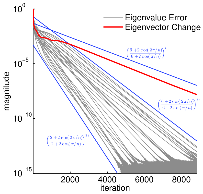
Figure 7: The convergence behavior of the power method in the circulant algebra. The gray lines show the error in the each eigenvalue in Fourier space. These curves track the predictions made based on the eigenvalues as discussed in the text. The red line shows the magnitude of the change in the eigenvector. We use this as the stopping criteria. It also decays as predicted by the ratio of eigenvalues. The blue fit lines have been visually adjusted to match the behavior in the convergence tail.

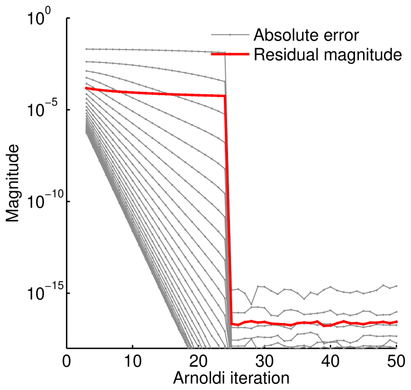
Figure 8: The convergence behavior of a GMRES procedure using the circulant Arnoldi process. The gray lines show the error in each Fourier component and the red line shows the magnitude of the residual. We observe poor convergence in one Fourier component; until the Arnoldi basis captures all of the eigenvalues after $N/2+1=26$ iterations. These results show how the two computations are performing individual power methods or Arnoldi processes in Fourier space.

8 Summary

We have extended the circulant algebra, introduced by Kilmer et al. (2008), with new operations to pave the way for iterative algorithms, such as the power method and the Arnoldi iteration that we introduced. These operations provided key tools to build a Matlab package to investigate these iterative algorithms for this paper. Furthermore, we used the fast Fourier transform to accelerate these operations, and as a key analysis tool for eigenvalues and eigenvectors. In the Fourier space the operations and algorithms decouple into individual problems. We observed this for the inner product, eigenvalues, eigenvectors, the power method, and the Arnoldi iteration. We also found that this decoupling explained the behavior in a numerical example.

Given that decoupling is such a powerful computational and analytical tool, a natural question that arises is when it is useful to employ the original circulant formalism, rather than work in the Fourier space. For dense computations, it is likely that working entirely in Fourier space is a superior approach. However, for sparse computations, such as the system $\ushort{\boldsymbol{A}}\circ\ushort{\mathbf{u}}=\ushort{\mathbf{f}}$ explored in Section 7, such a conclusion is unwarranted. That example is sparse both in the matrix over circulants, and in the individual circulant arrays. When thought of as a cube of data, it is sparse in any way of slicing it into a matrix. After this matrix $\ushort{\boldsymbol{A}}$ is transformed to the Fourier space, it loses its sparsity in the third-dimension; each sparse scalar $\ushort{A}_{i,j}$ becomes a dense array. In this case, retaining the coupled nature of the operations and even avoiding most of the Fourier domain may allow better scalability in terms of total memory usage.

An interesting topic for future work is exploring other rings besides the ring of circulants. One obvious candidate is the ring of symmetric circulant matrices. In this ring, the Fourier coefficients are always real-valued. Using this ring avoids the algebraic and computational complexity associated with complex values in the Fourier transforms.

We have made all of code and experiments available to use and reproduce our results: http://stanford.edu/~dgleich/publications/2011/codes/camat.

References

Appendix A The circulant scalar magnitude

This section describes another operation we extended to the circulant algebra. Eventually, we replaced it with our ordering (Definition 4), which is more powerful as we justify below. However, it plays a role in our Matlab package, and thus we describe the rationale for our choice of magnitude function here.

For scalars in $\mathbb{R}$, the magnitude is often called the absolute value. Let $\alpha,\beta\in\mathbb{R}$. The absolute value has the the property $\left|\alpha\beta\right|=\left|\alpha\right|\left|\beta\right|$. We have already introduced an absolute value function, however. Here, we wish to define a notion of magnitude that produces a scalar in $\mathbb{R}$ to indicate the size of an element. Such a function will have norm-like flavor because it must represent the aggregate magnitude of $k$ values with a single real-valued number. Thus, finding a function to satisfy $\left|\ushort{\alpha}\circ\ushort{\beta}\right|=\left|\ushort{\alpha}\right|\left|\ushort{\beta}\right|$ exactly is not possible. Instead, we seek a function $g:\mathbb{K}_{k}\mapsto\mathbb{R}$ such that

1. $g(\ushort{\alpha})=0$ if and only if $\ushort{\alpha}=0$,

2. $g(\ushort{\alpha}\circ\ushort{\beta})\leq g(\ushort{\alpha})g(\ushort{\beta})$,

3. $g(\ushort{\alpha}+\ushort{\beta})\leq g(\ushort{\alpha})+g(\ushort{\beta})$.

The following result shows that there is a large class of such magnitude functions.

Result 1.

Any sub-multiplicative matrix norm $\left\|\boldsymbol{A}\right\|$ defines a magnitude function $g(\ushort{\alpha})=\left\|\operatorname{\texttt{circ}}(\ushort{\alpha})\right\|.$

This result follows because the properties of the function $g$ are identical to the requirements of a sub-multiplicative matrix norm applied to $\operatorname{\texttt{circ}}(\ushort{\alpha})$. Any matrix norm induced by a vector norm is sub-multiplicative. In particular, the matrix $1$, $2$, and $\infty$ norms are all sub-multiplicative. Note that for circulant matrices both the matrix $1$ and $\infty$ norms are equal to the 1-norm of any row or column, i.e., $\left\|\operatorname{\texttt{vec}}(\alpha)\right\|_{1}$ is a valid magnitude. Surprisingly, the 2-norm of the vector of parameters, that is $\left\|\operatorname{\texttt{vec}}(\ushort{\alpha})\right\|_{2}$, is not. For a counterexample, let $\ushort{\alpha}=\left\{\!\begin{smallmatrix}1&2\end{smallmatrix}\!\right\},\ushort{\beta}=\left\{\!\begin{smallmatrix}2&4\end{smallmatrix}\!\right\}$. Then $\ushort{\alpha}\circ\ushort{\beta}=\left\{\!\begin{smallmatrix}8&10\end{smallmatrix}\!\right\}$ and $\left\|\operatorname{\texttt{vec}}(\ushort{\alpha}\circ\ushort{\beta})\right\|_{2}=\sqrt{164}>\left\|\operatorname{\texttt{vec}}(\ushort{\alpha})\right\|_{2}\left\|\operatorname{\texttt{vec}}(\ushort{\beta})\right\|_{2}=\sqrt{100}.$ For many practical computations, we use the matrix $2$-norm of $\operatorname{\texttt{circ}}(\ushort{\alpha})$ as the magnitude function. Thus,

$$\left|\ushort{\alpha}\right|\equiv\left\|\operatorname{\texttt{circ}}(\ushort{\alpha})\right\|_{2}=\left\|\operatorname{\texttt{cft}}(\ushort{\alpha})\right\|_{1}.$$

This choice has the following relationship with our ordering:

$$\operatorname{\texttt{abs}}(\ushort{\alpha})\leq\operatorname{\texttt{abs}}(\ushort{\beta})\qquad\Rightarrow\qquad\left|\ushort{\alpha}\right|\leq\left|\ushort{\beta}\right|.$$

We implement this operation as the mag function in our Matlab package.

References

- Arnoldi (1951) Arnoldi, W. E., 1951. The principle of minimized iterations in the solution of the matrix eigenvalue problem. Quarterly of Applied Mathematics 9, 17–29.
- Baker (1989) Baker, J. R., 1989. Macrotasking the singluar value decomposition of block circulant matrices on the cray-2. In: Proceedings of the 1989 ACM/IEEE conference on Supercomputing. Supercomputing ’89. ACM, New York, NY, USA, pp. 243–247.
- Braman (To appear) Braman, K., To appear. Third order tensors as linear operators on a space of matrices. Linear Algebra Appl. URL http://www.mcs.sdsmt.edu/kbraman/Research/Teigs2-submitted.pdf
- Brewer et al. (1986) Brewer, J. W., Bunce, J. W., Vleck, F. S., 1986. Linear systems over commutative rings. Vol. 104 of Lecture notes in pure and applied mathematics. Marcel Dekker. URL http://books.google.com/books?id=xddbW1kj4zYC
- Chu and Watterson (1993) Chu, M. T., Watterson, J. L., September 1993. On a multivariate eigenvalue problem, part i: algebraic theory and a power method. SIAM J. Sci. Comput. 14, 1089–1106. URL http://portal.acm.org/citation.cfm?id=159930.159936
- Davis (1979) Davis, P. J., 1979. Circulant matrices. Wiley.
- De Mazancourt and Gerlic (1983) De Mazancourt, T., Gerlic, D., September 1983. The inverse of a block-circulant matrix. Antennas and Propagation, IEEE Transactions on 31 (5), 808–810. URL http://ieeexplore.ieee.org/xpls/abs_all.jsp?arnumber=1143132&ta%g=1
- Granata et al. (1992) Granata, J., Conner, M., Tolimieri, R., January 1992. The tensor product: a mathematical programming language for FFTs and other fast DSP operations. IEEE Signal Processing Magazine 9 (1), 40–48.
- Gurvits et al. (1992) Gurvits, L., Rodman, L., Shalom, T., July 1992. Controllability and completion of partial upper triangular matrices over rings. Linear Algebra and its Applications 172, 135–149. URL http://www.sciencedirect.com/science/article/B6V0R-45F5VYC-CS/2%/25906e8df1f7a763fd1c37b3f900f8e9
- Gustafson (1979) Gustafson, W. H., February 1979. Roth’s theorems over commutative rings. Linear Algebra and its Applications 23, 245–251. URL http://www.sciencedirect.com/science/article/B6V0R-45FKGH1-9R/2%/c5ca43747018e55b16f944f31a4d014e
- Gustafson (1991) Gustafson, W. H., November 1991. Modules and matrices. Linear Algebra and its Applications 157, 3–19. URL http://www.sciencedirect.com/science/article/B6V0R-45FKGCC-7B/2%/40b933213ad066898d57a74cc5cf5284
- Hafner and McCurley (1991) Hafner, J. L., McCurley, K. S., December 1991. Asymptotically fast triangularization of matrices over rings. SIAM J. Comput. 20 (6), 1068–1083.
- Higham (2008) Higham, N. J., 2008. Functions of Matrices: Theory and Computation. SIAM.
- Kilmer et al. (2008) Kilmer, M. E., Martin, C. D., Perrone, L., 2008. A third-order generalization of the matrix svd as a product of third-order tensors. Tech. Rep. TR-2008-4, Tufts University. URL http://www.cs.tufts.edu/tech_reports/reports/2008-4/report.pdf
- Kolda and Bader (2009) Kolda, T. G., Bader, B. W., August 2009. Tensor decompositions and applications. SIAM Review 51 (3), 455–500. URL http://link.aip.org/link/?SIR/51/455/1
- Krylov (1931) Krylov, A. N., 1931. On the numerical solution of the equation by which in technical questions frequencies of small oscillations of material systems are determined (russian). Izv. Akad. Nauk SSSR VII (4), 491–539.
- Lambert (1996) Lambert, R. H., May 1996. Multichannel blind deconvolution: FIR matrix algebra and separation of multipath mixtures. Ph.D. thesis, University of Southern California.
- Lambert et al. (2001) Lambert, R. H., Joho, M., Mathis, H., December 2001. Polynomial singular values for number of wideband sources estimation and principal component analysis’. In: International Conference on Independent Component Analysis and Blind Signal Separation ICA. pp. 379–383. URL http://ica-bss.org/joho/research/publications/ica_01.pdf
- Lanczos (1950) Lanczos, C., October 1950. An iteration method for the solution of the eigenvalue problem of linear differential and integral operators. Journal of Research of the National Bureau of Standards 45 (4), 255–282. URL http://nvl.nist.gov/pub/nistpubs/jres/045/4/V45.N04.A01.pdf
- Mcdonald (1984) Mcdonald, B. R., 1984. Linear algebra over commutative rings. No. 87 in Pure and applied mathematics. Marcel Dekker.
- Navasca et al. (2010) Navasca, C., Opperman, M., Penderghest, T., Tamon, C., 2010. Tensors as module homomorphisms over group rings. arXiv 1005.1894, 1–11. URL http://arxiv.org/abs/1005.1894
- Prasad (1994) Prasad, K. M., November 1994. Generalized inverses of matrices over commutative rings. Linear Algebra and its Applications 211, 35–52. URL http://www.sciencedirect.com/science/article/B6V0R-45DHWPS-H/2/%90bdae2d4c656d3bc1a2fa23478193e1
- Qi (2007) Qi, L., January 2007. Eigenvalues and invariants of tensors. Journal of Mathematical Analysis and Applications 325 (2), 1363 – 1377. URL http://www.sciencedirect.com/science/article/B6WK2-4JK4PNS-5/2/%4dcb0914917df6344bf71f709d1afe1f
- Saad (2003) Saad, Y., 2003. Iterative Methods for Sparse Linear Systems, 2nd Edition. Society for Industrial and Applied Mathematics, Philadelphia.
- Sinnott and Harrington (1973) Sinnott, D., Harrington, R., Sep 1973. Analysis and design of circular antenna arrays by matrix methods. Antennas and Propagation, IEEE Transactions on 21 (5), 610–614.
- Sontag (1976) Sontag, E. D., 1976. Linear systems over commutative rings: A survey. Ricerche di Automatica 1, 1–34.
- Stewart (2001) Stewart, G. W., 2001. Eigensystems. Vol. 2 of Matrix Algorithms. SIAM, Philadelphia. URL http://books.google.com/books?id=Y3k5TNTnEmEC
- Tee (2005) Tee, G. J., 2005. Eigenvectors of block circulant and alternating circulant matrices. Research Letters in the Information and Mathematical Sciences 8, 123–142. URL http://iims.massey.ac.nz/research/letters/volume8/tee/tee.pdf
- Vescovo (1997) Vescovo, R., Oct 1997. Inversion of block-circulant matrices and circular array approach. Antennas and Propagation, IEEE Transactions on 45 (10), 1565–1567.
- von Mises and Pollaczek-Geiringer (1929) von Mises, R., Pollaczek-Geiringer, H., 1929. Praktische verfahren der gleichungsauflösung. Zeitschrift für Angewandte Mathematik und Mechanik 9 (2), 152–164.