Generalized Parton Distributions and Their Singularities

Abstract

A new approach to building models of generalized parton distributions (GPDs) is discussed that is based on the factorized DD (double distribution) Ansatz within the single-DD formalism. The latter was not used before, because reconstructing GPDs from the forward limit one should start in this case with a very singular function $f(\beta)/\beta$ rather than with the usual parton density $f(\beta)$. This results in a non-integrable singularity at $\beta=0$ exaggerated by the fact that $f(\beta)$’s, on their own, have a singular $\beta^{-a}$ Regge behavior for small $\beta$. It is shown that the singularity is regulated within the GPD model of Szczepaniak et al., in which the Regge behavior is implanted through a subtracted dispersion relation for the hadron-parton scattering amplitude. It is demonstrated that using proper softening of the quark-hadron vertices in the regions of large parton virtualities results in model GPDs $H(x,\xi)$ that are finite and continuous at the “border point” $x=\xi$. Using a simple input forward distribution, we illustrate implementation of the new approach for explicit construction of model GPDs. As a further development, a more general method of regulating the $\beta=0$ singularities is proposed that is based on the separation of the initial single DD $f(\beta,\alpha)$ into the “plus” part $[f(\beta,\alpha)]_{+}$ and the $D$-term. It is demonstrated that the “DD+D” separation method allows to (re)derive GPD sum rules that relate the difference between the forward distribution $f(x)=H(x,0)$ and the border function $H(x,x)$ with the $D$-term function $D(\alpha)$.

I Introduction

The ongoing and future experimental studies of Generalized Parton Distributions (GPDs) Mueller et al. (1994); Ji (1997); Radyushkin (1996); Collins et al. (1997) require theoretical models for GPDs which satisfy several nontrivial requirements, such as polynomiality Ji (1998), positivity Martin and Ryskin (1998); Pire et al. (1999); Radyushkin (1999) hermiticity Mueller et al. (1994), time reversal invariance Ji (1998), etc., following from the most general principles of quantum field theory. In particular, the polynomiality requirement, which states that the $x^{n}$ moment of a GPD $H(x,\xi;t)$ is a polynomial in $\xi$ of the order not higher than $n+1$, is a consequence of the Lorentz invariance. The polynomiality condition is automatically satisfied when GPDs are constructed from Double Distributions (DDs) Mueller et al. (1994); Radyushkin (1996, 1996, 1999), (see also ), thus the problem of constructing a model for a GPD converts into a problem of building a model for the relevant DD $F(\beta,\alpha;t)$.

Since a DD $F(\beta,\alpha;t)$ has hybrid properties: it behaves like a usual parton distribution function (PDF) with respect to $\beta$, as a meson distribution amplitude (DA) with respect to $\alpha$, and as a form factor with respect to the invariant momentum transfer $t$, it was proposed Radyushkin (1999, 1999) (in the simplified formal $t=0$ limit) to build a model DD $F(\beta,\alpha)$ as a product of the usual PDF $f(\beta)$ and a profile function $h(\beta,\alpha)$ that has an $\alpha$-shape of a meson DA. This construction allows one to get an intuitive feeling about the shape of GPDs and their change with the change of the skewness parameter $\xi$. It was noticed Polyakov and Weiss (1999), however, that in the case of isosinglet GPDs, such a Factorized DD Ansatz (FDDA) does not produce the highest, $(n+1)^{\rm st}$ power of $\xi$ in the $x^{n}$ moment of $H(x,\xi)$. To cure this problem, a “two-DD” parameterization was proposed Polyakov and Weiss (1999), with the second DD $G(\beta,\alpha)$ capable of generating, among others, the required $\xi^{n+1}$ power. It was also proposed Polyakov and Weiss (1999) to use a “DD plus D” parameterization in which the second DD $G(\beta,\alpha)$ is reduced to a function $D(\alpha)$ of one variable, the D-term , that is solely responsible for the $\xi^{n+1}$ contribution. The importance of the $D$-term and its physical interpretation was studied in further works (see Ref. Goeke et al. (2001) and references therein).

Later, it was found out that it is still possible to write a “single-DD” parameterization Belitsky et al. (2001) that incorporates just one function, but produces all the required powers up to $\xi^{n+1}$. This representation also has a remarkable property that it allows, in principle, to invert the GPD/DD relation, i.e., to obtain DD if GPD is known. So far, however, the single-DD representation was not used for building models for GPDs using the factorized DD Ansatz. The reason is that one should use much more singular function $f(\beta)/\beta$ rather than just the usual PDF $f(\beta)$ for the GPD reconstruction from the forward limit. The combination $f(\beta)/\beta$, being an even function in the singlet case, has a non-integrable singularity at $\beta=0$, even if $f(\beta)$ is finite at $\beta=0$. Furthermore, the fact that PDFs $f(\beta)$ have a singular $\beta^{-a}$ Regge behavior makes the problem even worse.

In an independent development Szczepaniak et al. (2009), an attempt was made to implant the Regge behavior into a GPD model constructed in the spirit of the covariant parton model Landshoff et al. (1971), with the hadron-parton transition amplitude written in the dispersion relation representation capable of generating the desired $s^{a}$ Regge behavior through an appropriately chosen spectral density. To handle $a>0$, the subtracted dispersion relation was used. The outcome was the claim Szczepaniak et al. (2009) that the GPDs $H(x,\xi)$ in this model have a singular $(x-\xi)^{-a}$ behavior in the vicinity of the “border” point $x=\xi$, which, if true, would ruin the applicability of the perturbative QCD formalism employing GPDs, since the latter works only when the GPDs are finite and continuous across the border point $x=\xi$.

Our starting goal was to examine the model of Ref. Szczepaniak et al. (2009) and to pinpoint the physical assumptions that resulted in the prediction of the singular $(x-\xi)^{-a}$ behavior (for an earlier analysis, see Ref. Kumericki et al. (2007)). As our analysis shows, the singularity follows from the use of the point-like approximation for the hadron-parton vertices. For bound states, however, one expects that the hadron wave function would generate an additional power-like (or even exponential) suppression in the regions where the parton virtuality $k^{2}$ is large. We found, that if such a suppression is properly included in the model, the resulting GPDs are finite and continuous for $x=\xi$.

In our study, we also observed that the expression for GPDs derived from the model of Ref. Szczepaniak et al. (2009) corresponds to a single-DD representation. Moreover, it has the structure of a factorized DD Ansatz, but with the singularity at $\beta=0$ regularized by the subtraction made in the dispersion relation for the quark-hadron scattering amplitude. Thus, the model of Ref. Szczepaniak et al. (2009) (corrected for an appropriate softening of the hadron-parton vertices) gives a framework for building GPD models within the single-DD scheme. Using a simple, but rather realistic model for the input forward distribution (i.e., usual PDF), we illustrate, step by step, how to use this framework for the construction of GPDs.

In particular, we found that the model produces a $D$-term contribution, despite the fact that it uses only the forward distribution as an input. The formal reason is that the subtraction introduced in the dispersion relation differs from the subtraction that converts the original DD $f(\beta,\alpha)$ into a (mathematical) “plus” distribution $[f(\beta,\alpha)]_{+}$, which, by definition, cannot generate a $D$-term. This observation raises the questions of a general nature about the separation of the $D$-term from the initial DD $f(\beta,\alpha)$ of the single-DD formalism.

We found that the separation of $f(\beta,\alpha)$ into the “plus” part $[f(\beta,\alpha)]_{+}$ and the $D$-term can be used to rederive the sum rule Teryaev (2005); Anikin and Teryaev (2007); Kumericki et al. (2008); Diehl and Ivanov (2007); Teryaev (2010) related to the dispersion relation for the real part of the DVCS amplitude Teryaev (2005); Anikin and Teryaev (2007); Kumericki et al. (2008); Diehl and Ivanov (2007); Teryaev (2010), and we also gave the derivation of another sum rule Anikin and Teryaev (2007) proposed as the $\xi\to 0$ limit of that generic sum rule, and which relates the difference between the forward distribution $f(x)=H(x,0)$ and the border function $H(x,x)$ with the $D$-term function $D(\alpha)$.

The paper is organized as follows. To make it self-contained, we start, in Sect. II, with a short review of the basic facts about DDs and GPDs. In Sect. III, we describe the model Szczepaniak et al. (2009) with implanted Regge behavior, and give our derivation of expressions for GPDs and DDs that follow from this model. We stress the necessity of a profile function that eliminates the singularities for $x=\xi$ and present explicit results for models with two simplest non-flat profiles. In Sect. IV, we perform a model-independent study of GPD sum rules, using the procedure of separating the initial DD into its “plus” part and the $D$-term. We emphasize that $H(x,0)/x$ and $H(x,x)/x$, due to their singular nature, should be treated as (mathematical) distributions rather than functions. Finally, we summarize the paper.

II Preliminaries

II.1 Double distributions

Generalized parton distributions (GPDs) Mueller et al. (1994); Ji (1997); Radyushkin (1996); Collins et al. (1997) naturally appear in the perturbative QCD description of the deeply virtual Compton scattering (DVCS) Ji (1997),Radyushkin (1996) (for reviews see Ji (1998); Radyushkin (2000); Goeke et al. (2001); Diehl (2003); Belitsky and Radyushkin (2005); Boffi and Pasquini (2007)), the process in which a highly virtual photon with momentum $q$, upon scattering on a hadron converts into a real photon with momentum $q^{\prime}=q+r$. Basic features of GPD construction, in fact, are not specific to QCD, and may be illustrated on examples of simpler theories Radyushkin (1998). In a toy scalar model (scalar quarks $\psi$ interacting with a scalar photon $\phi$ through $\psi\psi\phi$ vertex), the lowest-order (handbag) diagram (see Fig.1) may be written, in the coordinate representation, as

$$C(q,P,r) =\int{\cal D}(z)e^{-i(qz)/2-i(q^{\prime}z)/2}$$

$$\times \langle P-r/2|\psi(z/2)\psi(-z/2)|P+r/2\rangle\,d^{4}z\ ,$$ (1)

where $z$ is the separation between the “photon” vertices, and $P=(p+p^{\prime})/2$ is the average of the initial $p$ and the final $p^{\prime}$ momenta of the struck hadron, and ${\cal D}(z)$ is the quark propagator.

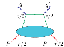
Figure 1: Structure of the handbag diagram for deeply virtual Compton scattering.

The matrix element may depend on the coordinate difference $z$ through invariants $(Pz),(rz)$ and $z^{2}$ only. For large $Q^{2}=-q^{2}$, the higher terms of the $z^{2}$ expansion have $1/Q^{2}$ suppression, thus the leading power term is generated from the matrix element taken at $z^{2}=0$. The extraction of the $z^{2}=0$ part of the matrix element may be performed in the standard way: through Taylor expansion in $z$ followed by taking only the symmetric-traceless part (denoted by $\{\ \}$)

$$\psi(0)\{\stackrel{{\scriptstyle\leftrightarrow}}{{\partial}}_{\mu_{1}}\ldots\stackrel{{\scriptstyle\leftrightarrow}}{{\partial}}_{\mu_{n}}\}\psi(0)$$

of the resulting local operators. For a scalar target, one may write

$$\langle P+r/2|\psi(0)\{\stackrel{{\scriptstyle\leftrightarrow}}{{\partial}}_{\mu_{1}}\ldots\stackrel{{\scriptstyle\leftrightarrow}}{{\partial}}_{\mu_{n}}\}\psi(0)|P-r/2\rangle$$

$$=\sum_{n=0}^{\infty}\biggl{[}\sum_{l=0}^{n-1}A_{nl}\{P_{\mu_{1}}\ldots P_{\mu_{n-l}}r_{\mu_{n-l+1}}\ldots r_{\mu_{n}}\}$$

$$+A_{nn}\{r_{\mu_{1}}\ldots r_{\mu_{n}}\}\biggr{]}\ .$$ (2)

In the momentum representation, the derivative $\stackrel{{\scriptstyle\leftrightarrow}}{{\partial}}_{\mu}\$ converts into the average $\bar{k}_{\mu}=(k_{\mu}+k^{\prime}_{\mu})/2$ of the initial $k$ and final $k^{\prime}$ quark momenta. After integration over $k$, $(\bar{k})^{n}$ should produce the $P$ and $r$ factors in the r.h.s. of the equation above. In this sense, one may treat $(\bar{k})^{n}$ as $(\beta P+\alpha r/2)^{n}$ and define the double distribution (DD) Mueller et al. (1994); Radyushkin (1996, 1996, 1999)

$$\frac{n!}{(n-l)!\,l!\,2^{l}}\int_{\Omega}F(\beta,\alpha)\beta^{n-l}\alpha^{l}\,d\beta\,d\alpha=A_{nl}$$ (3)

as a function whose $\beta^{n-l}\alpha^{l}$ moments are proportional to the coefficients $A_{nl}$. It can be shown Mueller et al. (1994); Radyushkin (1996, 1999) that the support region $\Omega$ is given by the rhombus $|\alpha|+|\beta|\leq 1$. These definitions result in the “DD parameterization”

$$\langle P-r/2|\psi(-z/2)\psi(z/2)|P+r/2\rangle$$

$$=\int_{\Omega}F(\beta,\alpha)\,e^{-i\beta(Pz)-i\alpha(rz)/2}\,d\beta\,d\alpha+{\cal O}(z^{2})\ .$$ (4)

of the matrix element.

II.2 Generalized parton distributions

Substituting the DD parameterization of the matrix element into the expression for the Compton amplitude, one obtains

$$C(q,P,r)=\int_{\Omega}F(\beta,\alpha)\,D\left[q+\beta P+\frac{1+\alpha}{2}r\right]\,d\beta\,d\alpha\ ,$$ (5)

where $D[l]$ is the quark propagator in the momentum representation. Thus, the leading-twist term corresponds to a parton picture in which the initial quark carries momentum $\beta P+(1+\alpha)r/2$. Neglecting $P^{2},(Pr)$ and $r^{2}$, we get

$$(q+\beta P+(1+\alpha)r/2)^{2}=-Q^{2}+2\beta(Pq^{\prime})+(1+\alpha)(rq^{\prime})\ ,$$

i.e., $\beta$ and $\alpha$ appear in the propagator in the combination $\beta(Pq^{\prime})+\alpha(rq^{\prime})/2$ only. The latter may be written as $x(Pq^{\prime})$, with $x=\beta+\xi\alpha$, where $\xi=(rq^{\prime})/2(Pq^{\prime})$. This redefinition leads to the parton picture in which the initial quark carries momentum $(x+\xi)P$. Introducing the generalized parton distribution (GPD) Mueller et al. (1994); Ji (1997); Radyushkin (1996)

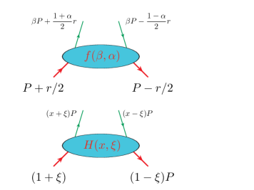
Figure 2: Parton picture in terms of DDs and in terms of GPDs.

$$H(x,\xi)=\int_{\Omega}F(\beta,\alpha)\,\delta(x-\beta-\xi\alpha)\,d\beta\,d\alpha\ ,$$ (6)

one can write the handbag contribution as

$$T(q,P,r)=\int_{-1}^{1}H(x,\xi)\,D\bigl{(}q+(x+\xi)P\bigr{)}\,dx\ .$$ (7)

One may try to define GPDs directly:

$$\langle P+r/2|\psi(-z/2)\psi(z/2)|P-r/2\rangle$$

$$=\int_{-1}^{1}\,e^{-ix(Pz)}H(x,\xi)\,dx+{\cal O}(z^{2})\ .$$ (8)

However, an immediate question is what is the skewness $\xi$ in this definition? It cannot be treated as the ratio of $(rz)/2$ and $(Pz)$, since the ratio $(rz)/2(Pz)$ cannot be the same for all points $z$. Hence, it is impossible to straightforwardly use such a definition in the expression (1) involving a 4-dimensional integration over $z$. But, if one uses the DD parametrization and integrates over $z$, then the scalar products $(Pz)$ and $(rz)$ convert into the scalar products $(Pq^{\prime})$ and $(rq^{\prime})$, respectively, since all other invariants, $P^{2},r^{2},(Pr)$ are neglected when they appear in the ratios with $(Pq^{\prime})$, $(rq^{\prime})$ or $Q^{2}$ . In this sense, only the $q^{\prime}$ part of $z$ is visible in the final result, and one may define GPDs by the formula (8) in which $z$ is substituted by a light-like vector $n$ proportional to $q^{\prime}$, say, by $n_{\mu}=q^{\prime}_{\mu}/2(Pq^{\prime})$.

Still, the appearance of process-dependent quantities like $(rq^{\prime})$ and $(Pq^{\prime})$ in the definition of GPDs confronts the basic idea of the factorization approach that the parton distributions are process-independent functions. The standard “escape” is that $(rq^{\prime})/(Pq^{\prime})$ in the GPD definitions is substituted by an apparently “process-neutral” ratio $r^{+}/P^{+}$, supplied by information that $P$ basically defines the “plus direction” and that some vector $n$ defines the “minus direction” (for DVCS, $n\sim q^{\prime}$). But this procedure creates a wrong impression that the definition of GPDs requires a reference to a particular frame. As shown above, one can define GPDs $H(x,\xi)$ through formulas (4), (6), which do not refer to any particular frame or process, and $\xi$ is just some parameter. Of course, for each particular process, $\xi$ should be adjusted to the kinematics of the process, e.g., $\xi=(rq^{\prime})/2(Pq^{\prime})$ for DVCS. Also, the parton interpretation of GPDs has the most natural form in the frame, where $P$ for a massless hadron (and $t=0$) defines the plus direction.

II.3 $D$-term

II.3.1 Scalar quarks

Parameterizing the matrix element (2), one may wish to separate the $A_{nn}$ terms that are accompanied by tensors built from the momentum transfer vector $r$ only (and, thus, invisible in the forward $r=0$ limit), and introduce the $D$-term Polyakov and Weiss (1999)

$$\int_{-1}^{1}D(\alpha)\,(\alpha/2)^{n}\,d\alpha=A_{nn}$$ (9)

as a function whose $(\alpha/2)^{n}$ moments give $A_{nn}$. Within the DD-parameterization, the separation of the $D$-term can be made by simply using $e^{-i\beta(Pz)}=[e^{-i\beta(Pz)}-1]+1$. The $D$-term is then given by

$$D(\alpha)=\int_{-1+|\alpha|}^{1-|\alpha|}F(\beta,\alpha)\,d\beta\ ,$$ (10)

and the DD-parameterization converts into a “DD plus D” parameterization

$$\langle P-r/2|\psi(-z/2)\psi(z/2)|P+r/2\rangle$$

$$=\int_{\Omega}[F(\beta,\alpha)]_{+}\,e^{-i\beta(Pz)-i\alpha(rz)/2}\,d\beta\,d\alpha$$

$$+\int_{-1}^{1}D(\alpha)\,e^{-i\alpha(rz)/2}\,d\alpha+{\cal O}(z^{2})\ ,$$ (11)

where

$$[F(\beta,\alpha)]_{+}=F(\beta,\alpha)-\delta(\beta)\int_{-1+|\alpha|}^{1-|\alpha|}F(\gamma,\alpha)\,d\gamma\ .$$ (12)

is the DD with subtracted $D$-term. Mathematically, $[F(\beta,\alpha)]_{+}$ is a “plus distribution” with respect to $\beta$. It satisfies the condition

$$\int_{-1+|\alpha|}^{1-|\alpha|}[F(\beta,\alpha)]_{+}\,d\beta=0\ ,$$ (13)

guaranteeing that no $D$-term can be constructed from $[F(\beta,\alpha)]_{+}$.

II.3.2 Spin-1/2 quarks: two-DD representation

In the simple model with scalar quarks discussed above, one may just use the original DD $F(\beta,\alpha)$ without splitting it into the “plus” part and the $D$-term. In models with spin-1/2 quarks, it is more difficult to avoid an explicit introduction of extra functions producing a $D$-term. The basic reason Polyakov and Weiss (1999) is that the matrix element of the bilocal operator in that case should have two parts

$$\langle P-r/2|\bar{\psi}(-z/2)\gamma_{\mu}\psi(z/2)|P+r/2\rangle|_{\rm twist-2}$$

$$=2P_{\mu}f\bigl{(}(Pz),(rz),z^{2}\bigr{)}+r_{\mu}g\bigl{(}(Pz),(rz),z^{2}\bigr{)}\ .$$ (14)

This suggests to introduce a parametrization with two DDs corresponding to $f$ and $g$ functions Polyakov and Weiss (1999). For the matrix element (14) multiplied by $z^{\mu}$ – which is exactly what one obtains doing the leading-twist factorization for the Compton amplitude Balitsky and Braun (1989) – this gives

$$z^{\mu}\langle P-r/2|\bar{\psi}(-z/2)\gamma_{\mu}\psi(z/2)|P+r/2\rangle$$

$$=\int_{\Omega}e^{-i\beta(Pz)-i\alpha(rz)/2}\,\biggl{[}2(Pz)F(\beta,\alpha)$$

$$+(rz)G(\beta,\alpha)\biggr{]}\,d\beta\,d\alpha\ +{\cal O}(z^{2}).$$ (15)

The separation into $F$- and $G$-parts in this case is not unique: expanding the exponential in powers of $(Pz)$ and $(rz)$, one may obtain the same $(Pz)^{m}(rz)^{l}$ term both from the $F$-type and $G$-type parts. This leads to possibility of “gauge transformations” Teryaev (2001): one can change

$$F(\beta,\alpha) \to F(\beta,\alpha)+\partial\chi(\beta,\alpha)/\partial\alpha\ ,$$ (16)

$$G(\beta,\alpha) \to G(\beta,\alpha)-\partial\chi(\beta,\alpha)/\partial\beta\ ,$$ (17)

using a gauge function $\chi(\beta,\alpha)$ that is odd in $\alpha$. Still, the terms $(Pz)^{0}(rz)^{l}$ cannot be produced from the $F$-type contribution. The maximum of what can be done is to absorb all $m\neq 0$ contributions into the $F$-type term. As a result, Eq. (15) is converted into a “DD plus D” parameterization Polyakov and Weiss (1999) in which the term in the square brackets is substituted by the

$$2(Pz)F_{D}(\beta,\alpha)+(rz)\delta(\beta)D(\alpha)$$ (18)

combination, with $D(\alpha)$ given by the $\beta$-integral of $G(\beta,\alpha)$ and $F_{D}(\beta,\alpha)$ related to the original DDs through the gauge transformation with

$$\chi_{D}(\beta,\alpha)=\frac{1}{2}\left\{\int_{-\beta}^{\beta}G(\gamma,\alpha)\,d\gamma-\int_{-1+|\alpha|}^{1-|\alpha|}G(\gamma,\alpha)\,d\gamma\right\}$$ (19)

(cf. Teryaev (2001); Tiburzi (2004)).

II.3.3 Spin-1/2 quarks: single-DD representation

In fact, since the Dirac index $\mu$ is symmetrized in the local twist-two operators $\bar{\psi}\{\gamma_{\mu}\stackrel{{\scriptstyle\leftrightarrow}}{{\partial}}_{\mu_{1}}\ldots\stackrel{{\scriptstyle\leftrightarrow}}{{\partial}}_{\mu_{n}}\}\psi$ with the $\mu_{i}$ indices related to the derivatives, one may expect that it also produces the factor $\beta P_{\mu}+\alpha r_{\mu}/2$. As shown by the authors of Ref. Belitsky et al. (2001), this is precisely what happens. In their construction, not only the exponential produces the $z$-dependence in the combination $\beta(Pz)+\alpha(rz)/2$, but also the pre-exponential terms come in the $\beta(Pz)+\alpha(rz)/2$ combination, i.e., the result is a representation in which

$$2(Pz)F(\beta,\alpha)+(rz)G(\beta,\alpha)$$

$$=[2\beta(Pz)+\alpha(rz)]f(\beta,\alpha)\ ,$$ (20)

that corresponds to $F(\beta,\alpha)=\beta f(\beta,\alpha)$ and $G(\beta,\alpha)=\alpha f(\beta,\alpha)$. Thus, formally, one deals with just one DD $f(\beta,\alpha)$. In principle, though, this single function may be a sum of several components, e.g., $\delta(\alpha)f(\beta)/\beta+\delta(\beta)D(\alpha)/\alpha$ (the result of the pioneering $D$-term paper Polyakov and Weiss (1999) for the pion DD in an effective chiral model corresponds to $f^{I=0}(\beta,\alpha)=\delta(\alpha)/|\beta|-\delta(\beta)/|\alpha|$).

In the two-DD approach, GPDs are introduced through

$$H(x,\xi)=\int_{\Omega}\bigl{[}F(\beta,\alpha)+\xi G(\beta,\alpha)\bigr{]}\,\delta(x-\beta-\xi\alpha)\,d\beta\,d\alpha\ ,$$ (21)

which converts into

$$H(x,\xi) =\int_{\Omega}(\beta+\xi\alpha)f(\beta,\alpha)\,\delta(x-\beta-\xi\alpha)\,d\beta\,d\alpha$$

$$=x\int_{\Omega}f(\beta,\alpha)\,\delta(x-\beta-\xi\alpha)\,d\beta\,d\alpha$$ (22)

in the “single-DD” formulation. The $D$-term in the single-DD case is given by

$$D(\alpha)=\alpha\int_{-1+|\alpha|}^{1-|\alpha|}f(\beta,\alpha)\,d\beta\ ,$$ (23)

and one may write $f(\beta,\alpha)$ as a sum

$$f(\beta,\alpha)=[f(\beta,\alpha)]_{+}+\delta(\beta)\frac{D(\alpha)}{\alpha}$$ (24)

of its “plus” part

$$[f(\beta,\alpha)]_{+}=f(\beta,\alpha)-\delta(\beta)\int_{-1+|\alpha|}^{1-|\alpha|}f(\gamma,\alpha)\,d\gamma$$ (25)

and $D$-term part $\delta(\beta){D(\alpha)}/{\alpha}$.

Despite the fact that the “plus” part and the $D$-term are obtained from the same DD $f(\beta,\alpha)$, they are independent in the sense that the “plus” part does not contribute in Eq. (23), and the $D$-term contribution drops from Eq. (25).

II.3.4 Getting GPDs from DDs

The forward limit $r=0$ corresponds to $\xi=0$, and GPD $H(x,\xi)$ converts into the usual parton distribution $f(x)$. Using DDs, we may write

$$f(x) =\int_{-1+|x|}^{1-|x|}F(x,\alpha)\,d\alpha=x\int_{-1+|x|}^{1-|x|}f(x,\alpha)\,d\alpha\ .$$ (26)

Thus, the forward distributions $f(x)$ are obtained by integrating DDs over vertical lines $\beta=x$ in the $(\beta,\alpha)$ plane. For nonzero $\xi$, GPDs are obtained from DDs through integrating them along the lines $\beta=x-\xi\alpha$ having $1/\xi$ slope, i.e. the family of $H(x,\xi)$ functions for different values of $\xi$ is obtained by “scanning” the same DD at different angles.

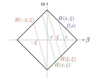
Figure 3: Support region for double distributions and lines producing $f(x),H(x,\xi)$ (for $x>\xi$ and $x<\xi$), $H(\xi,\xi)$ and $H(-\xi,\xi)$.

For $x>\xi>0$, the integration lines lie completely inside the right half of the rhombus. The line producing GPD at the “border” point $x=\xi$ starts at its upper corner, while the lines corresponding to $|x|<\xi$ cross the line $\beta=0$. Thus, one deals with the “outer” regions $x>\xi$ and $x<-\xi$ (in this case, the whole line is in the left half of the rhombus) and the central region $-\xi<x<\xi$, when the integration lines in the $(\beta,\alpha)$ plane lie in both halves of the rhombus and intersect the $\beta=0$ line.

In GPD variables $(x,\xi)$, the momentum fraction $x-\xi$ carried by the final quark is positive for the right outer region, and negative for the central region, i.e., in the latter case it should be interpreted as an outgoing antiquark rather than incoming quark Radyushkin (1996), i.e. GPD in the central region describes emission of a quark-antiquark pair with total plus momentum $r^{+}$ shared in fractions $(1+x/\xi)/2$ and $(1-x/\xi)/2$, like in a meson distribution amplitude.

From this physical interpretation, one may expect that the behavior of a GPD $H(x,\xi)$ in the central region is unrelated to that in the outer region. But, since the GPD in both regions is obtained from the same DD, one may expect, to the contrary, that the set of GPDs for all “outer” $x$’s and all $\xi$’s contains the same information as the set of GPDs for all central $x$’s and all $\xi$’s. This “holographic” picture (cf. Kumericki et al. (2008, 2008)) may be violated by terms contributing to GPDs in the central region and not contributing to GPDs in the outer regions: the terms with support on the $\beta=0$ line, i.e., those proportional to $\delta(\beta)$ (and, in principle, its derivatives), in particular, the $D$-term. For this reason, the usual approach is to build separate models for the $D$-term and for the remaining part of DD.

II.3.5 Factorized DD Ansatz

The reduction formula (26) suggests a model

$$f(\beta,\alpha)=\frac{f(\beta)}{\beta}h(\beta,\alpha)\ ,$$ (27)

where $f(\beta)$ is the forward distribution, while $h(\beta,\alpha)$ determines DD profile in the $\alpha$ direction and satisfies the normalization condition

$$\int_{-1+|\beta|}^{1-|\beta|}h(\beta,\alpha)\,d\alpha=1\ .$$ (28)

Since the plus component of the momentum transfer $r$ is shared between the quarks in fractions $(1+\alpha)/2$ and $(1-\alpha)/2$, like in a meson distribution amplitude, it was proposed Radyushkin (1999, 1999) to model the shape of the profile function by

$$h_{N}(\beta,\alpha)\sim\frac{[(1-|\beta|)^{2}-\alpha^{2}]^{N}}{(1-|\beta|)^{2N+1}}\ ,$$ (29)

with $N$ being a parameter governing the width of the profile.

Such a factorized DD Ansatz (FDDA) was originally Radyushkin (1999, 1999) applied to an analog of the $F(\beta,\alpha)$ function of the two-DD formalism, which corresponds to a model $F(\beta,\alpha)=f(\beta)h(\beta,\alpha)$ and $G(\beta,\alpha)=0$. Later, it was corrected by addition of the $D$-term Polyakov and Weiss (1999), which formally corresponds to the “gauge” (19) in which $G(\beta,\alpha)\to G_{D}(\beta,\alpha)=\delta(\beta)D(\alpha)$, and $F(\beta,\alpha)\to F_{D}(\beta,\alpha)$. Note that if $F=\beta f$ and $G=\alpha f$, the model $F_{D}(\beta,\alpha)=f(\beta)\,h(\beta,\alpha)$ does not coincide with the model $f(\beta,\alpha)=f(\beta)\,h(\beta,\alpha)/\beta$, since the gauge function $\chi_{D}(\beta,\alpha)$ (see Eq. (16)) is nontrivial.

Thus, there is a question whether the FDDA should be applied to $F_{D}(\beta,\alpha)$ (as it was done so far) or to the DD $f(\beta,\alpha)$ of the single-DD formulation. It should be confessed that no enthusiasm has been observed to use FDDA in the form of the single-DD formula (27). This observation has a simple explanation: the function $f(\beta)/\beta$ is not integrable for $\beta=0$, even if $f(\beta)$ is finite for $\beta=0$. The reason is that the DVCS amplitude contains singlet GPDs, which are odd functions of $\beta$. Hence, $f(\beta)/\beta$ should be an even function, and the principal value prescription does not work. Moreover, for small $\beta$ one would expect that the forward distribution $f(\beta)$ has a singular $f(\beta)\sim 1/\beta^{a}$ Regge behavior, which makes the problem even worse.

III GPD model with implanted Regge behavior

III.1 Formulation

The assumptions used in the factorized DD Ansatz are based on the experience with calculating DDs for triangle diagrams Radyushkin (1998) and form factors in the light-front formalism models with power-law dependence of the wave function on transverse momentum Mukherjee et al. (2003) (see also Hwang and Mueller (2008)).

The simplest triangle diagram (see Fig.4) in the scalar model corresponding to Eq. (2) may be used as an example of a model for GPD

$$H(x,\xi)\sim\int\frac{d^{4}k\,\delta(x-(kn)/(Pn))}{(m_{1}^{2}-k_{1}^{2})(m_{2}^{2}-k_{2}^{2})(m_{3}^{2}-(P-k)^{2})}\ .$$ (30)

Though the $\xi$-dependence is not immediately visible here, it appears after integration over $k$ through the $(rn)/2(Pn)$ ratio. The DD $F(\beta,\alpha)$ generated by this diagram is just a constant Radyushkin (1997), which corresponds to a flat $N=0$ profile $h_{0}(\beta,\alpha)\sim 1/(1-\beta)$ and $f(\beta)\sim 1-\beta$ forward distribution.

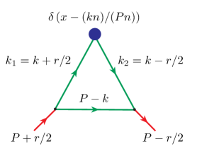
Figure 4: Triangle diagram model for GPD.

The calculation Mukherjee et al. (2003) of overlap integrals for light-front wave functions with a power-law behavior $\psi(x,k_{\perp})\sim 1/(k_{\perp}^{2})^{1+\kappa}$ resulted in expressions equivalent to using DDs with $N=\kappa$ profile in Eq. (29) and forward distributions behaving like $(1-\beta)^{2\kappa+1}$. The same profile arises Mukherjee et al. (2003) if one differentiates a scalar triangle diagram $\kappa$ times with respect to masses (squared) of each active quark.

The triangle diagrams, however, do not generate the Regge $f(\beta)\sim 1/\beta^{a}$ behavior for small $\beta$. The latter may be obtained, in particular, by infinite summation of higher-order $t$-channel ladder diagrams (see, e.g., Efremov and Radyushkin (2009)). A simpler way was proposed in Ref. Szczepaniak et al. (2009), where the spectator propagator was substituted by a parton-hadron scattering amplitude $T(P,r,k)$ (see Fig.5) written in the dispersion relation representation. To avoid divergencies generated by the Regge behavior, the subtracted dispersion relation

$$T(P,r,k)\to T((P-k)^{2})=T_{0}$$

$$+\int_{0}^{\infty}d\sigma{\rho(\sigma)\,}\left\{\frac{1}{\sigma-(P-k)^{2}}-\frac{1}{\sigma}\right\}$$ (31)

was used. The spectral function $\rho(\sigma)$ here should be adjusted to produce a desired Regge-type behavior with respect to $s=(P-k)^{2}$ .

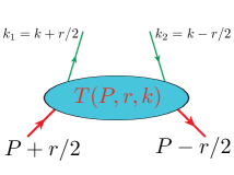
Figure 5: Hadron-quark scattering amplitude.

In the light-front formalism, the starting contribution corresponds to a triangle diagram in which the hadron-quark vertices are substituted by the light-front wave functions $\psi(x,k_{\perp})$ that bring in an extra fall-off of the integrand at large transverse momenta $k_{\perp}$. The authors of Ref. Szczepaniak et al. (2009) intended to reflect this physics in their covariant model. To introduce form factors bringing in a faster fall-off of the $k$-integrand with respect to quark virtualities $k_{1}^{2}$ and $k_{2}^{2}$, it was proposed to use higher powers of $1/(m_{i}^{2}-k_{i}^{2})$ instead of perturbative propagators, which may be achieved by differentiating the triangle diagram with respect to $m_{i}^{2}$.

The model of Ref. Szczepaniak et al. (2009) assumes spin-1/2 quarks. It was argued that the Dirac structure of the hadron-parton scattering amplitude in this case should be given by $\not{k}$, which provides EM gauge invariance of the DVCS amplitude. Summarizing, the model scattering amplitude has the following structure

$$\,\frac{\not{k}\ T((P-k)^{2}}{(m_{1}^{2}-k_{1}^{2})^{N_{1}+1}(m_{2}^{2}-k_{2}^{2})^{N_{2}+1}}\ .$$ (32)

To treat the two quarks on equal footing, it makes sense to take $m_{1}=m_{2}$, but we will keep them different for a while, to separate effects produced by nonzero $N_{1}$ and $N_{2}$.

After $\not{k}$ is contracted with the $\not{n}$ factor from the operator vertex, one gets $(kn)$, and the model GPD that will be analyzed below is given by

$$H(x,\xi)=\frac{1}{\pi^{2}}\frac{N_{1}!N_{2}!}{(N_{1}+N_{2})!} \int\frac{(kn)}{(Pn)}\frac{d^{4}k\,\delta(x-(kn)/(Pn))}{[m_{1}^{2}-(k+r)^{2}]^{N_{1}+1}[m_{2}^{2}-(k-r)^{2}]^{N_{2}+1}}\left[T_{0}+\int_{0}^{\infty}d\sigma{\rho(\sigma)\,}\left\{\frac{1}{\sigma-(P-k)^{2}}-\frac{1}{\sigma}\right\}\right]\ .$$ (33)

The overall factors were introduced here for future convenience. Using the $\alpha$-representation

$$\frac{N!}{(m^{2}-k^{2})^{N+1}}=\int_{0}^{i\infty}e^{\alpha(k^{2}-m^{2})}\alpha^{N}\,d\alpha\hskip 28.45274pt,\hskip 28.45274pt\frac{1}{\sigma}=\int_{0}^{i\infty}e^{-\alpha_{3}\sigma}\,d\alpha_{3}$$ (34)

for propagators and also for the $1/\sigma$ subtraction term gives

$$\frac{x}{(N_{1}+N_{2})!} \int_{0}^{\infty}d\sigma\,\rho(\sigma)\int_{0}^{i\infty}{\alpha_{1}^{N_{1}}d\alpha_{1}\,\alpha_{2}^{N_{2}}d\alpha_{2}\,d\alpha_{3}}\,\left\{\delta\left(x-\frac{\alpha_{3}+(\alpha_{2}-\alpha_{1})(rn)/2(Pn)}{\alpha_{1}+\alpha_{2}+\alpha_{3}}\right)\frac{1}{(\alpha_{1}+\alpha_{2}+\alpha_{3})^{2}}\right.$$

$$\left.-\delta\left(x-\frac{(\alpha_{2}-\alpha_{1})(rn)/(Pn)}{\alpha_{1}+\alpha_{2}}\right)\,\frac{1}{(\alpha_{1}+\alpha_{2})^{2}}\right\}e^{-\alpha_{3}\sigma-\alpha_{1}m_{1}^{2}-\alpha_{2}m_{2}^{2}}$$ (35)

for the terms involved in the dispersion integral. The second delta-function corresponds to the $1/\sigma$ subtraction term of the dispersion representation. It is accompanied by the $1/(\alpha_{1}+\alpha_{2})^{2}$ factor because $1/\sigma$ does not have $k$-dependence. Introducing the skewness variable $\xi\equiv(rn)/2(Pn)$, changing $\alpha_{i}\equiv x_{i}\lambda$ and integrating over $\lambda$ we obtain

$$x\int_{0}^{\infty}d\sigma\,\rho(\sigma) \int_{0}^{1}\frac{x_{1}^{N_{1}}dx_{1}\,x_{2}^{N_{2}}dx_{2}\,dx_{3}\,\delta(1-x_{1}-x_{2}-x_{3})}{(x_{3}\sigma+x_{1}m_{1}^{2}+x_{2}m_{2}^{2})^{N_{1}+N_{2}+1}}\left\{\delta\left(x-x_{3}-{(x_{2}-x_{1})\xi}\right)-\frac{\delta\left(x-{(x_{2}-x_{1})\xi}\right)}{(x_{1}+x_{2})^{2}}\right\}\ .$$ (36)

Taking equal masses $m_{1}=m_{2}\equiv m$, using $x_{1}+x_{2}=(1-x_{3})$ and introducing $z$ through $x_{1}=(1-x_{3})z$ results in

$$x\int_{0}^{\infty}d\sigma\,\rho(\sigma) \int_{0}^{1}dx_{3}\,dz\,\frac{(1-x_{3})^{N_{1}+N_{2}+1}z^{N_{1}}(1-z)^{N_{2}}\,}{[x_{3}\sigma+(1-x_{3})m^{2}]^{N_{1}+N_{2}+1}}\left\{\delta\bigl{(}x-x_{3}-{(x_{2}-x_{1})\xi}\bigr{)}-\frac{\delta\left(x-{(x_{2}-x_{1})\xi}\right)}{(1-x_{3})^{2}}\right\}\ .$$ (37)

The $T_{0}$ subtraction term gives the $D$-term-type contribution

$$D_{0}(x/\xi)=\frac{T_{0}}{2^{N_{1}+N_{2}}(N_{1}+N_{2})}\left(\frac{x}{|\xi|}\right)\left(1-\frac{x}{\xi}\right)^{N_{1}}\left(1+\frac{x}{\xi}\right)^{N_{2}}\,\theta\left(\left|\frac{x}{\xi}\right|<1\right)$$ (38)

that vanishes outside the central region and, hence, is invisible in the forward limit. In what follows, we will concentrate on the terms generated by the dispersion integral, but one should remember that the $D_{0}$ term can always be added to GPD $H(x,\xi)$, i.e., in all formulas below one should be ready to change $H(x,\xi)\to H(x,\xi)+D_{0}(x/\xi)$.

III.2 Forward case

The case $\xi=0$ corresponds to the forward distribution

$$H(x,\xi=0)=x\int_{0}^{\infty}d\sigma\,\rho(\sigma) \int_{0}^{1}dx_{3}\,dz\,\frac{(1-x_{3})^{N_{1}+N_{2}+1}z^{N_{1}}(1-z)^{N_{2}}\,}{[x_{3}\sigma+(1-x_{3})m^{2}]^{N_{1}+N_{2}+1}}\left\{\delta(x-x_{3})-\frac{\delta(x)}{(1-x_{3})^{2}}\right\}\ .$$ (39)

Taking $x\delta(x)=0$ for $x\neq 0$ gives

$$H(x,\xi=0)= \frac{N_{1}!N_{2}!}{(N_{1}+N_{2}+1)!}\,x\,(1-x)^{N_{1}+N_{2}+1}\int_{0}^{\infty}\frac{d\sigma\,\rho(\sigma)}{(x\sigma+(1-x)m^{2})^{N_{1}+N_{2}+1}}\equiv f(x)\ .$$ (40)

Formally, we may also write

$$\frac{H(x,\xi=0)}{x}=\frac{f(x)}{x}-{\delta(x)}\int_{0}^{1}dx_{3}\,\frac{f(x_{3})}{x_{3}(1-x_{3})^{2}}$$ (41)

The second term provides the subtraction regularizing the function $f(x)/x$ at its singular point $x=0$.

III.3 DD description

In the double distribution representation, we have $x=\beta+\alpha\xi$. So, turning back to Eq. (36) and changing there $1-x_{1}-x_{2}\equiv\beta$, $x_{2}-x_{1}\equiv\alpha$, we obtain that

$$x_{1}=\frac{1}{2}(1-\beta-\alpha)\ \ ,\ \ x_{2}=\frac{1}{2}(1-\beta+\alpha)\ ,$$ (42)

which gives for equal masses

$$\frac{x}{2^{N_{1}+N_{2}+1}}\int_{0}^{\infty}d\sigma\,\rho(\sigma) \int_{0}^{1}d\beta\int_{-1+\beta}^{1-\beta}d\alpha\,\frac{(1-\beta-\alpha)^{N_{1}}\,(1-\beta+\alpha)^{N_{2}}}{(\beta\sigma+(1-\beta)m^{2})^{N_{1}+N_{2}+1}}\left\{\delta\left(x-\beta-\alpha\xi\right)-\frac{\delta\left(x-\alpha\xi\right)}{(1-\beta)^{2}}\right\}\ .$$ (43)

Thus, a faster decrease of the $k$-integrand with respect to the quark virtualities $k_{1}^{2}$ or $k_{2}^{2}$ results in a suppression of the DD behavior by powers of $(1-\beta-\alpha)$ or $(1-\beta+\alpha)$ when $\alpha$ approaches the support boundary $|\alpha|=1-\beta$. For equal $N_{1}=N_{2}=N$, we obtain

$$\frac{x}{2^{2N+1}}\int_{0}^{\infty}d\sigma\,\rho(\sigma) \int_{0}^{1}d\beta\int_{-1+\beta}^{1-\beta}d\alpha\,\frac{[(1-\beta)^{2}-\alpha^{2}]^{N}\,}{(\beta\sigma+(1-\beta)m^{2})^{2N+1}}\left\{\delta\left(x-\beta-\alpha\xi\right)-\frac{\delta\left(x-\alpha\xi\right)}{(1-\beta)^{2}}\right\}\ .$$ (44)

Using Eq.(40), one can substitute the $\sigma$-integral through forward distribution to get

$$H(x,\xi)=\frac{x}{2^{2N+1}}\frac{(2N+1)!}{(N!)^{2}} \int_{0}^{1}d\beta\,\int_{-1+\beta}^{1-\beta}d\alpha\,\frac{[(1-\beta)^{2}-\alpha^{2}]^{N}\,}{(1-\beta)^{2N+1}}\,\frac{f(\beta)}{\beta}\left\{\delta\left(x-\beta-\alpha\xi\right)-\frac{\delta\left(x-\alpha\xi\right)}{(1-\beta)^{2}}\right\}\ .$$ (45)

This trick allows one to by-pass the question about the specific form of the spectral density $\rho(\sigma)$.

It is easy to notice that the factor

$$h_{N}(\beta,\alpha)\equiv\frac{1}{2^{2N+1}}\frac{(2N+1)!}{(N!)^{2}}\frac{[(1-\beta)^{2}-\alpha^{2}]^{N}\,}{(1-\beta)^{2N+1}}$$ (46)

is precisely a normalized profile satisfying

$$\int_{-1+\beta}^{1-\beta}h_{N}(\beta,\alpha)\,d\alpha=1\ .$$ (47)

Since $x_{1}+x_{2}\leq 1$ for the Feynman parameters $x_{1},x_{2}$, we have $\beta\geq 0$ in the expressions above. The $\beta\leq 0$ part of DD comes from the crossed diagram, in which the dispersion relation is written for $T((P+k)^{2})$. For the singlet case, the full DD $f(\beta,\alpha)$ should be symmetric with respect to interchange $\beta\to-\beta$ (and also symmetric under $\alpha\to-\alpha$), which results in GPD $H(x,\xi)$ that is an odd function of $x$. For this reason, we will proceed with the $\beta\geq 0$ case, keeping in mind to antisymmetrize the resulting $H(x,\xi)$ at the very end.

Thus, we can rewrite Eq.(45) as

$$\frac{H(x,\xi)}{x}= \int_{0}^{1}d\beta\,\int_{-1+\beta}^{1-\beta}d\alpha\,\frac{f(\beta)}{\beta}\,h_{N}(\beta,\alpha)\,\left\{\delta\left(x-\beta-\alpha\xi\right)-\frac{\delta\left(x-\alpha\xi\right)}{(1-\beta)^{2}}\right\}\ .$$ (48)

The first term

$$\frac{H^{(1)}(x,\xi)}{x}=\int_{0}^{1}d\beta\,\int_{-1+\beta}^{1-\beta}d\alpha\,\frac{f(\beta)}{\beta}\,h_{N}(\beta,\alpha)\,\delta\left(x-\beta-\alpha\xi\right)$$ (49)

coincides with the factorized DD Ansatz for $H(x,\xi)/x$ in which it is reconstructed from its forward limit $f(x)/x$. The relevant double distribution is given by $f(\beta,\alpha)=h_{N}(\beta,\alpha){f(\beta)}/{\beta}$. The second term may be rewritten as

$$\frac{H^{(2)}(x,\xi)}{x}=-\int_{0}^{1}d\beta\,\int_{-1+\beta}^{1-\beta}d\alpha\,\delta\left(x-\beta-\alpha\xi\right)\,\delta(\beta)\int_{0}^{1-|\alpha|}d\gamma\,\frac{f(\gamma,\alpha)}{(1-\gamma)^{2}}\,,$$ (50)

and it provides a regularization of the $\beta$-integral in Eq. (45). The total contribution is given by

$$\frac{H(x,\xi)}{x} =\int_{0}^{1}d\beta\,\int_{-1+\beta}^{1-\beta}d\alpha\,\delta\left(x-\beta-\alpha\xi\right)$$

$$\times \left\{f(\beta,\alpha)-\delta(\beta)\int_{0}^{1-|\alpha|}d\gamma\,\frac{f(\gamma,\alpha)}{(1-\gamma)^{2}}\right\}\ .$$ (51)

Thus, the model of Ref. Szczepaniak et al. (2009), first, corresponds to the single-DD representation (22), and, second, it has the structure of the factorized DD Ansatz (27). Furthermore, due to the subtraction in the dispersion relation (31), one deals with the regularized double distribution

$$f^{\rm reg}(\beta,\alpha)=f(\beta,\alpha)-\delta(\beta)\int_{0}^{1-|\alpha|}d\gamma\,\frac{f(\gamma,\alpha)}{(1-\gamma)^{2}}\ .$$ (52)

Returning back to Eq.(48) and calculating integral over $\alpha$, we formally obtain

$$H(x,\xi)=\frac{x}{\xi}\,\theta(x>\xi)\int_{\beta_{1}}^{\beta_{2}}d\beta\,\frac{f(\beta)}{\beta}\,h(\beta,(x-\beta)/\xi)$$

$$+\frac{x}{\xi}\,\theta(|x|<\xi)\int_{0}^{\beta_{2}}d\beta\,\frac{f(\beta)}{\beta}\,h(\beta,(x-\beta)/\xi)$$

$$-\frac{x}{\xi}\,\theta(|x|<\xi)\int_{0}^{1-|x|/\xi}d\beta\,\frac{f(\beta)}{\beta(1-\beta)^{2}}\,h(\beta,x/\xi)\ ,$$ (53)

where (see Fig. 6)

$$\beta_{1}=\frac{x-\xi}{1-\xi}\ ,\beta_{2}=\frac{x+\xi}{1+\xi}\ .$$ (54)

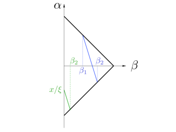
Figure 6: Support region and integration lines producing $H(x,\xi)$ for $x>\xi$ and $x<\xi$ from a double distribution that is nonzero for $\beta>0$ only.

One should realize, however, that the second and the third integrals diverge and should be combined together to regularize their singularity at $\beta=0$. This may be achieved by rewriting the $|x|<\xi$ part in the form

$$H(x,\xi)|_{|x<\xi}=\frac{x}{\xi}\,\int_{0}^{\beta_{2}}d\beta\,\frac{f(\beta)}{\beta}\,\bigl{[}h(\beta,(x-\beta)/\xi)-h(\beta,x/\xi)\bigr{]}$$

$$+\frac{x}{\xi}\,\int_{0}^{\beta_{2}}d\beta\,\frac{f(\beta)}{\beta}\,h(\beta,x/\xi)\left(1-\frac{1}{(1-\beta)^{2}}\right)$$

$$-\frac{x}{\xi}\,\int_{\beta_{2}}^{1-|x|/\xi}d\beta\,\frac{f(\beta)}{\beta(1-\beta)^{2}}\,h(\beta,x/\xi)$$ (55)

explicitly showing the compensation of the $1/\beta$ factor.

III.4 Results

III.4.1 $N=1$ profile

For the model forward distribution

$$f_{a}(\beta)={(1-\beta)^{3}}/{\beta^{a}}$$ (56)

and the profile function

$$h_{1}(\beta,\alpha)=\frac{3}{4}\,\frac{(1-\beta)^{2}-\alpha^{2}}{(1-\beta)^{3}}\ ,$$ (57)

we obtain, for $x>\xi$:

$$H(x,\xi)|_{x>\xi}= \frac{3}{4}\,\frac{x}{\xi}\int_{\beta_{1}}^{\beta_{2}}\frac{d\beta}{\beta^{a+1}}\left\{(1-\beta)^{2}-\left(\frac{x-\beta}{\xi}\right)^{2}\right\}\ .$$ (58)

Calculating $H(\xi,\xi)$, i.e., the GPD at the border point $x=\xi$, one gets here the $[(1-\beta)^{2}-(1-\beta/\xi)^{2}]\sim\beta$ factor from the profile function, and this factor changes the strength of singularity for $\beta=0$. As a result, the integral over $\beta$ converges as far as $a<1$. This outcome is a consequence of using a profile function that linearly vanishes at the sides of the support rhombus. In its turn, the $N=1$ profile is generated by the assumed $1/(k_{1}^{2}k_{2}^{2})^{2}$ dependence of the $k$-integrand for large parton virtualities. If one takes the $N=0$ profile, the factor in the curly brackets should be substituted by $1/(1-\beta)$), and the integral producing $H(\xi,\xi)$ diverges. For small, but nonzero $x-\xi$, one obtains the behavior proportional to $1/\beta_{1}^{a}\sim(x-\xi)^{-a}$. This result is similar to that obtained in Ref. Szczepaniak et al. (2009). However, since its authors explicitly declared that they are going to soften the hadron-quark vertices by differentiating the diagram over the quark masses, one may wonder, how did it happen that they obtained a singular result?

The subtlety is that they took equal quark masses $m_{1}=m_{2}=m$ from the very beginning, and used differentiation with respect to this common $m^{2}$. Here it should be noted that because

$$\left(\frac{d}{dm^{2}}\right)^{2} \frac{1}{(m^{2}-k_{1}^{2})(m^{2}-k_{2}^{2})}=\frac{1}{(m^{2}-k_{1}^{2})^{3}(m^{2}-k_{2}^{2})}+\frac{2}{(m^{2}-k_{1}^{2})^{2}(m^{2}-k_{2}^{2})^{2}}+\frac{1}{(m^{2}-k_{1}^{2})(m^{2}-k_{2}^{2})^{3}}\ ,$$ (59)

the first and the third term on the r.h.s. are not softened with respect to one of the virtualities, i.e., one of the hadron-parton vertices remains pointlike. As we have seen above, imposing the $1/(k_{1}^{2})^{N_{1}+1}(k_{2}^{2})^{N_{2}+1}$ dependence on virtualities one would obtain the $(1-\beta-\alpha)^{N_{1}}(1-\beta+\alpha)^{N_{2}}/2^{N_{1}+N_{2}}$ factor, i.e., every differentiation with respect to $m_{1}^{2}$ gives $(1-\beta-\alpha)/2$, while every differentiation with respect to $m_{2}^{2}$ gives the $(1-\beta+\alpha)/2$ factor, both resulting in a nontrivial profile in the $\alpha$-direction. On the other hand, each differentiation with respect to the common $m^{2}$ gives the $(1-\beta-\alpha)/2+(1-\beta+\alpha)/2=(1-\beta)$ factor that has no dependence on $\alpha$. This kind of softening only increases the power of $(1-\beta)$, but DD remains flat in the $\alpha$-direction.

Note, that the use of $1/(k_{1}^{2})^{N+1}(k_{2}^{2})^{N+1}$-dependence in the model $D_{0}$-term contribution (38) results in the $(1-x^{2}/\xi^{2})^{N}$ factor, which gives $D_{0}(1)=0$ for $N>0$ case. This vanishing of $D_{0}(\alpha)$ at the end-points $\alpha=\pm 1$ has the same nature as the vanishing of the DDs at the sides of the support rhombus: both result from a faster than perturbative decrease of the $k$-integrand at large quark virtualities.

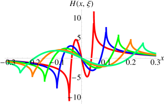
Figure 7: Model singlet GPD $H_{S}(x,\xi)$ with $N=1$ DD profile for $a=0.5$ and $\xi=0.05,0.1,0.15,0.2,0.25$.

Turning now to the $|x|<\xi$ region, we use Eq. (55) to represent the relevant term for the $N=1$ profile as

$$H(x,\xi)|_{|x|<\xi}= \frac{3}{4}\,\frac{x}{\xi}\left[\frac{1}{\xi^{2}}\int_{0}^{\beta_{2}}\frac{d\beta}{\beta^{a}}(2x-\beta)+\int_{0}^{\beta_{2}}\frac{d\beta}{\beta^{a}}\left\{1-\frac{x^{2}}{\xi^{2}(1-\beta)^{2}}\right\}(\beta-2)-\int_{\beta_{2}}^{1-|x|/\xi}\frac{d\beta}{\beta^{a+1}}\left\{1-\frac{x^{2}}{\xi^{2}(1-\beta)^{2}}\right\}\right]\ .$$ (60)

Note that as far as $|x|$ is strictly less than $\xi$, the profile function does not vanish at the singularity point $\beta=0$. The mechanism of softening singularity to $1/\beta^{a}$ strength is now provided by the $1/\sigma$ subtraction term of the original dispersion relation.

To get a model for singlet GPDs, one should take the antisymmetric combination

$$H_{S}(x,\xi)=H(x,\xi)-H(-x,\xi)\ .$$ (61)

The resulting GPDs are shown in Fig. 2. For positive $x$, they are peaking at $x=\xi$. The functions $H_{S}(x,\xi)$ in this model are continuous at $x=\pm\xi$, but the derivative $dH_{S}(x,\xi)/dx$ is discontinuous at these points.

III.4.2 $N=2$ Profile

Let us now take the $N=2$ profile function

$$h_{2}(\beta,\alpha)=\frac{15}{16}\,\frac{[(1-\beta)^{2}-\alpha^{2}]^{2}}{(1-\beta)^{5}}$$ (62)

and the same model forward distribution

$$f_{a}(\beta)=\frac{(1-\beta)^{3}}{\beta^{a}}\ .$$ (63)

For $x>\xi$ this gives

$$H(x,\xi)|_{x>\xi}= \frac{15}{16}\,\frac{x}{\xi}\int_{x_{1}}^{x_{2}}\frac{d\beta}{\beta^{a+1}(1-\beta)^{2}}\left[(1-\beta)^{2}-\left(\frac{x-\beta}{\xi}\right)^{2}\right]^{2}\ .$$ (64)

Evidently, the $N=2$ profile gives a $\sim\beta^{2}$ suppression, and $H(\xi,\xi)$ is finite as far as $a<2$.

Again, using Eq. (55), the $|x|<\xi$ term can be represented in the form

$$H(x,\xi)|_{|x|<\xi}= \frac{15}{16}\,\frac{x}{\xi^{5}}\int_{0}^{x_{2}}\frac{d\beta}{\beta^{a}}(2x-\beta)\left[\frac{x^{2}+(x-\beta)^{2}}{(1-\beta)^{2}}-2\xi^{2}\right]+\frac{15}{16}\,\frac{x}{\xi}\int_{0}^{x_{2}}\frac{d\beta}{\beta^{a}}\left[1-\frac{x^{2}}{\xi^{2}(1-\beta)^{2}}\right]^{2}(\beta-2)$$

$$-\frac{15}{16}\,\frac{x}{\xi}\int_{x_{2}}^{1-|x|/\xi}\frac{d\beta}{\beta^{a+1}}\left[1-\frac{x^{2}}{\xi^{2}(1-\beta)^{2}}\right]^{2}$$ (65)

explicitly showing the cancellation of the $1/\beta^{a+1}$ singularity.

The resulting GPDs are shown in Fig. 8. For positive $x$, they are peaking at points close to $x=\xi$. In the model with $N=2$ profile, both the functions $H_{S}(x,\xi)$ and their derivatives $dH_{S}(x,\xi)/dx$ are continuous at $x=\pm\xi$.

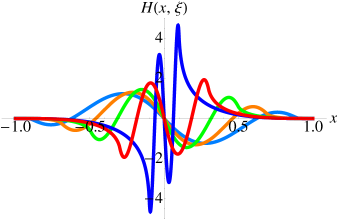
Figure 8: Model singlet GPD $H(x,\xi)$ with $N=2$ profile for $a=0.5$ and $\xi=0.1,0.3,0.5,0.7,0.9$.

III.5 $D$-term

The $\delta(\beta)$ subtraction term in the regularized DD (extended now onto the whole support rhombus)

$$f^{\rm reg}(\beta,\alpha)=f(\beta,\alpha)-\delta(\beta)\int_{-1+|\alpha|}^{1-|\alpha|}d\gamma\,\frac{f(\gamma,\alpha)}{(1-\gamma)^{2}}$$ (66)

softens the singularity of $f(\beta,\alpha)$ for $\beta=0$, but it does not convert $f(\beta,\alpha)$ into a “plus distribution” $[f(\beta,\alpha)]_{+}$ whose integral over $\beta$ vanishes. Thus, $f^{\rm reg}(\beta,\alpha)$ contains a nonzero $D$-term contribution

$$D(\alpha)= \alpha\int_{-1+|\alpha|}^{1-|\alpha|}f^{\rm reg}(\beta,\alpha)\,d\beta=\alpha\int_{-1+|\alpha|}^{1-|\alpha|}d\beta\,\frac{f(\beta)}{\beta}\,h(\beta,\alpha)\,\left\{1-\frac{1}{(1-|\beta|)^{2}}\right\}=2\alpha\int_{0}^{1-|\alpha|}d\beta\,{f(\beta)}\,h(\beta,\alpha)\,\frac{\beta-2}{(1-\beta)^{2}}\ .$$ (67)

Taking the same model forward distribution $f(\beta)={(1-\beta)^{3}}/{\beta^{a}}$ and $N=1$ profile function gives

$$D^{\{N=1\}}(\alpha)=\frac{3}{2}\,\alpha\int_{0}^{1-|\alpha|}\frac{d\beta}{\beta^{a}}\,\left[1-\frac{\alpha^{2}}{(1-\beta)^{2}}\right]\,(\beta-2)\ .$$ (68)

A similar expression for the $D$-term is obtained in the $N=2$ profile model:

$$D^{\{N=2\}}(\alpha)=\frac{15}{8}\,\alpha\int_{0}^{1-|\alpha|}\frac{d\beta}{\beta^{a}}\,\left[1-\frac{\alpha^{2}}{(1-\beta)^{2}}\right]^{2}\,(\beta-2)\ .$$ (69)

As one can see in Fig. 9, the two curves are rather close to each other.

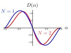
Figure 9: The $D$-terms in $N=1$ and $N=2$ profile models for $a=0.5$.

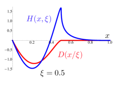
Figure 10: GPD $H(x,\xi)$ and $D$-term $D(x/\xi)$ for $\xi=0.5$ and positive $x$.

The comparison of the total GPD $H(x,\xi)$ and its $D$-term part is shown in Fig. 10.

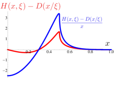
Figure 11: Difference between GPD $H(x,\xi)$ and $D$-term $D(x/\xi)$ in the case of the $N=1$ profile for $\xi=0.5$ and positive $x$. The same function divided by $x$ is also shown.

The difference between GPD $H(x,\xi)$ and $D$-term $D(x/\xi)$ corresponds to the term $H_{+}(x,\xi)$ obtained from the “plus” part $[f(\beta,\alpha)]_{+}$ of DD. The shape of the difference for $\xi=0.5$ is shown in Fig. 11. Note that, despite the fact that the forward distribution in this model is positive, there is a region, where the contribution to $H(x,\xi)$ coming from $[f(\beta,\alpha)]_{+}$ is negative. This is due to the $\delta(\beta)$ subtraction term contained in $[f(\beta,\alpha)]_{+}$. Also shown is the ratio $H_{+}(x,\xi)/x$. Looking at the figure, one may suspect that the $x$-integral of $H_{+}(x,\xi)/x$ vanishes. In the next section, we show that this, indeed, is the case.

IV GPD sum rules

IV.1 Formulation

The $D$-term determines the subtraction constant in the dispersion relation for the DVCS amplitude Teryaev (2005); Anikin and Teryaev (2007); Kumericki et al. (2008); Diehl and Ivanov (2007); Teryaev (2010). In particular, it was shown Anikin and Teryaev (2007) that the original expression for the real part of the DVCS amplitude involving $H(x,\xi)$, and the dispersion integral involving $H(x,x)$ differ by a constant $\Delta$ given by the integral of the $D$-term function $D(\alpha)$:

$$P\int_{-1}^{1}\frac{H(x,x)-H(x,\xi)}{x-\xi}\,dx=\Delta\equiv\int_{-1}^{1}\frac{D(\alpha)}{1-\alpha}\,d\alpha\ .$$ (70)

Here, $P$ denotes the principal value prescription. In Ref. Anikin and Teryaev (2007), this relation was derived using polynomiality properties of GPDs. It was also pointed out there that it can be obtained by incorporating representation of GPDs in the two-DD formalism (which is basically again the use of the polynomiality).

Taking $\xi=0$, one formally arrives at the sum rule

$$\int_{-1}^{1}\frac{H(x,x)-H(x,0)}{x}\,dx=\int_{-1}^{1}\frac{D(\alpha)}{1-\alpha}\,d\alpha\ .$$ (71)

Since both $H(x,0)/x$ and $H(x,x)/x$ are even functions of $x$, their singularities for $x=0$ cannot be regularized by the principle value prescription. Moreover, there are no indications that singularities of these two functions may cancel each other. On the contrary, as emphasized in Ref. Polyakov (2008), there are arguments that the ratio $H(x,x)/H(x,0)$ does not tend to 1 for small $x$.

The solution given in Refs. Kumericki et al. (2008, 2008); Polyakov and Semenov-Tian-Shansky (2009) is based on the analytic regularization of the $x$-integral. Namely, it is assumed that the positive Mellin moments (or conformal moments, see, e.g., Kumericki and Mueller (2010))

$$\Phi(j)\equiv\int_{-1}^{1}x^{j}[H(x,x)-H(x,0)]\,dx$$ (72)

can be analytically continued to the point $j=-1$. The result of such a procedure is equivalent to analytic regularization of the $x$-integral. However, the required analyticity properties of $\Phi(j)$ may be violated by singular or “invisible” terms (cf. Kumericki et al. (2008)) in the integrand of Eq.(72) (e.g., $x\delta(x)$ gives a non-analytic $\delta_{j,-1}$ contribution into $\Phi(j)$). In the model construction described above, singular terms explicitly appear as a result of subtractions in the dispersion relation, so our intention is to develop a less restrictive approach to this problem.

Below, we give a derivation of the sum rule (71 ) based on separation (25) of the DDs into the “plus” part and the $D$-term. No assumptions about smoothness will be made. In fact, the key element of the derivation is that $H(x,x)/x$ should be treated as a (mathematical) distribution at the point $x=0$ rather than a function. The same applies to $H(x,0)/x$.

IV.2 Ingredients

To begin with, we remind the basic formulas: the expression

$$\frac{H(x,\xi)}{x}=\int_{\Omega}f(\beta,\alpha)\,\delta(x-\beta-\xi\alpha)\,d\beta\,d\alpha$$ (73)

producing GPDs from DDs and the decomposition of DD

$$f(\beta,\alpha)=[f(\beta,\alpha)]_{+}+\delta(\beta)\frac{D(\alpha)}{\alpha}$$ (74)

into the “plus” part given by

$$[f(\beta,\alpha)]_{+}=f(\beta,\alpha)-\delta(\beta)\int_{-1+|\alpha|}^{1-|\alpha|}f(\gamma,\alpha)\,d\gamma$$ (75)

and the $D$-term part $\delta(\beta){D(\alpha)}/{\alpha}$.

Correspondingly, we split GPD into the part coming from the “plus” part of DD

$$\frac{H_{+}(x,\xi)}{x}\equiv \int_{\Omega}f(\beta,\alpha)\,\biggl{[}\delta(x-\beta-\xi\alpha)-\delta(x-\xi\alpha)\biggr{]}\,d\beta\,d\alpha$$ (76)

and that generated by the $D$-term

$$\frac{H_{D}(x,\xi)}{x}\equiv \int_{-1}^{1}\frac{D(\alpha)}{\alpha}\delta(x-\xi\alpha)\,d\alpha\ .$$ (77)

The latter integral gives an explicit expression

$$H_{D}(x,\xi)={\rm sign}(\xi)\,\theta(|x|<|\xi|)\,D(x/\xi)\ ,$$ (78)

but, as we will see, it is instructive to use the integral representation as well. Another important relation

$$\frac{H_{D}(x,0)}{x}= \delta(x)\int_{-1}^{1}\frac{D(\alpha)}{\alpha}\,d\alpha$$ (79)

is obtained by taking $\xi=0$.

Note, that if we take $x=\xi$, Eq. (78) gives

$$H_{D}(x,x)={\rm sign}(x)\,D(1)\ .$$ (80)

If $D(1)\neq 0$, then the integral for $\Delta$ in (70) diverges. However, as argued in the previous section, $D(1)=0$ for models with faster-than-perturbative decrease of the hadron-parton amplitude at large quark virtualities. Thus, we assume that $D(1)=0$, and furthermore that the integral of $D(\alpha)/(1-\alpha)$ converges. Then Eq. (77) gives

$$\frac{H_{D}(x,x)}{x}= \delta(x)\int_{-1}^{1}\frac{D(\alpha)}{\alpha(1-\alpha)}\,d\alpha\ .$$ (81)

The important point is that if we would use this formula to write an expression for $H_{D}(x,x)$ itself, we would get $x\delta(x)$ on the r.h.s., which should be treated as zero for integration with functions finite for $x=0$, since the coefficient given by the $\alpha$-integral is also finite. Thus, the scenario with $D(1)=0$ is self-consistent.

Note that both $H_{D}(x,0)/x$ and $H_{D}(x,x)/x$ are proportional to $\delta(x)$, with the coefficients given by integrals of $D(\alpha)$. This means that, unlike the functions $H(x,0)$ and $H(x,x)$, which, for $x\neq 0$, are insensitive to changes of $D(\alpha)$ in the $\delta(\beta)D(\alpha)/\alpha$ term, the (mathematical) distributions $H(x,0)/x$ and $H(x,x)/x$ contain information about such a $D$-term.

Our next step is to study contributions from different parts of the GPDs involved in the sum rule (71).

IV.3 “Secondary” sum rule

IV.3.1 “Plus” part

Forward function

One can easily see from Eq. (76) that

$$\int_{-1}^{1}\frac{H_{+}(x,\xi)}{x}\,dx=0$$ (82)

for any $\xi$, including $\xi=0$. Since the integrand is an even function of $x$, the vanishing of this integral means that we also have

$$\int_{0}^{1}\frac{H_{+}(x,\xi)}{x}\,dx=0\ .$$ (83)

Thus, $H_{+}(x,\xi)$ should be negative in some part of the central region, and this negative contribution should exactly compensate the contribution from the regions, where $H_{+}(x,\xi)$ is positive. In other words, on the $(0,1)$ interval, $H_{+}(x,\xi)/x$ has the same property as a “plus distribution” with respect to $x$. Note, that this does not mean that $H_{+}(x,\xi)/x$ necessarily contains singular functions like $\delta(x)$. For finite $\xi$, the function $H_{+}(x,\xi)/x$ is pretty regular for all $x$ values (see Fig.12). The negative $\delta(x)$ function appears only in the $\xi$=0 limit, i.e.

$$\frac{H_{+}(x,0)}{x}=\frac{f(x)}{x}-\delta(x)\int_{-1}^{1}\frac{f(y)}{y}\,dy\equiv\left[\frac{f(x)}{x}\right]_{+}\ .$$ (84)

(Here, it was taken into account that $H_{+}(x,0)$ coincides with the forward distribution $f(x)$ for $x\neq 0$).

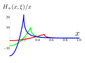
Figure 12: Function $H_{+}(x,\xi)/x$ in the model with the $N=1$ profile for $\xi=0.2,0.3,0.5$ and positive $x$.

Border function

For the integral involving the border function, we get

$$\int_{-1}^{1}\frac{H_{+}(x,x)}{x}\, dx=\int_{-1}^{1}dx\,\int_{\Omega}\,d\beta\,d\alpha\ {f(\beta,\alpha)}$$

$$\times \,\left[\delta\left(x(1-\alpha)-\beta\right)-\delta(x(1-\alpha))\right]\ .$$ (85)

Noting that equation $\alpha=1$ is satisfied in one point on the support region $\Omega$ only, namely, in the upper corner of the rhombus, we may treat $\delta(x(1-\alpha))$ as $\delta(x)/(1-\alpha)$ to get

$$\int_{-1}^{1}\frac{H_{+}(x,x)}{x}\,dx= \int_{-1}^{1}dx\,\int_{\Omega}\,d\beta\,d\alpha\ \frac{f(\beta,\alpha)}{1-\alpha}$$

$$\times\,\left[\delta\left(x-\frac{\beta}{1-\alpha}\right)-\delta(x)\right]\ .$$ (86)

Since $|\beta/(1-\alpha)|\leq 1$, the first $\delta$-function always works. As a result, the integrals coming from the two delta-functions cancel each other, and we have

$$\int_{-1}^{1}\frac{H_{+}(x,x)}{x}\,dx=0\ ,$$ (87)

just like for ${H_{+}(x,\xi)}/{x}$. Unlike $H_{+}(x,\xi)$, however, the combination $H_{+}(x,x)/x$ explicitly contains the $\delta(x)$ subtraction term, i.e. it is a genuine “plus distribution” with respect to $x$:

$$\frac{H_{+}(x,x)}{x}= \frac{H(x,x)}{x}-\delta(x)\int_{-1}^{1}\frac{H(y,y)}{y}\,dy$$

$$\equiv\left(\frac{H(x,x)}{x}\right)_{+}\ .$$ (88)

Summarizing, the “plus” parts of both functions entering into the sum rule (71) separately produce vanishing contributions into the $x$-integral. Furthermore, these zero contributions are due to the fact that $H_{+}(x,0)/x$ and $H_{+}(x,x)/x$ are “plus distributions”, which results in zero integrals irrespectively of the form of the forward distribution $f(x)$ and the border function $H(x,x)$.

IV.3.2 $D$-part

Let us now turn to the $D$-parts. First, we have

$$\int_{-1}^{1}\frac{H_{D}(x,\xi)}{x}\,dx= \int_{-1}^{1}\frac{D(\alpha)}{\alpha}\,d\alpha$$ (89)

for any fixed $\xi$, including $\xi=0$. This result may be obtained by integrating over $x$ the $\delta(x-\xi\alpha)$ factor in the integral representation (77). For non-vanising $\xi$, one can also use Eq. (78) in the $x$-integral and then change the integration variable through $x=\alpha\xi$.

For the integral involving the border function, we use Eq. (81), which gives

$$\int_{-1}^{1}\frac{H_{D}(x,x)}{x}\,dx{=} \int_{-1}^{1}\frac{D(\alpha)}{\alpha(1-\alpha)}\,d\alpha\ .$$ (90)

As a result,

$$\int_{-1}^{1}\frac{H_{D}(x,x)}{x}\,dx-\int_{-1}^{1}\frac{H_{D}(x,0)}{x}\,dx{=}\int_{-1}^{1}\frac{D(\alpha)}{1-\alpha}\,d\alpha\ .$$ (91)

Combining this outcome with zero contributions from the “plus” parts, one obtains the sum rule (71).

Thus, our construction confirms the sum rule. But our derivation shows that the “plus” parts of both terms simply do not contribute to the sum rule whatever the shapes of $f(x)$ and $H(x,x)$ are. Only the $D$-parts contribute, so there is no surprise that the net result can be expressed in terms of $D(\alpha)$.

An essential point is that both $H_{D}(x,0)/x$ and $H_{D}(x,x)/x$ are proportional to the $\delta(x)$-function, with the coefficients given by integrals of the $D$-term function $D(\alpha)$. In this sense, $H(x,0)/x$ and $H(x,x)/x$ “know” about the $D$-term.

A simple consequence is that all $x^{j}$ moments of $H_{D}(x,0)$ and $H_{D}(x,x)$ with $j\geq 0$ vanish and one cannot get the $D$-part of the sum rule (71) by an analytic continuation of the $x^{j}$ moments of $H_{D}(x,0)$ and $H_{D}(x,x)$ to $j=-1$, i.e., using the procedure of Refs.Kumericki et al. (2008, 2008); Polyakov and Semenov-Tian-Shansky (2009). In fact, $x^{j}$ moments of $H_{D}(x,0)$ and $H_{D}(x,x)$ are proportional to the Kronecker delta function $\delta_{j,-1}$.

IV.3.3 Formal derivation and need for renormalization

Since $H(x,0)/x$ is given by integrating the DD $f(\beta,\alpha)$ over $\alpha$ along vertical lines $\beta=x$, a subsequent integration over all $x$ gives DD $f(\beta,\alpha)$ integrated over the whole rhombus:

$$\int_{-1}^{1}\frac{H(x,0)}{x}\,dx {=}\int_{-1}^{1}dx\int_{\Omega}\,d\beta\,d\alpha f(\beta,\alpha)\delta(x-\beta)$$

$$=\int_{\Omega}f(\beta,\alpha)\,\,d\beta\,d\alpha=\int_{-1}^{1}\frac{D(\alpha)}{\alpha}\,d\alpha\ .$$ (92)

On the last step, we used that the $\beta$-integral of $f(\beta,\alpha)$ formally gives $D(\alpha)/\alpha$. However, if $f(\beta,\alpha)\sim 1/\beta^{{1+a}}$, being even in $\beta$, one needs a regularization for the $\beta$-integral. The “DD+D” separation (73), as we have seen, provides such a regularization. It works like a renormalization: the divergent integral formally giving the $D$-term is subtracted from the “bare” DD, and substituted by a finite “observable” function $D(\alpha)/\alpha$.

In a similar way, we can treat the second integral:

$$\int_{-1}^{1}\frac{H(x,x)}{x}\,dx {=}\int_{-1}^{1}dx\int_{\Omega}\,d\beta\,d\alpha f(\beta,\alpha)\delta(x-\beta-x\alpha)$$

$$= \int_{\Omega}\frac{f(\beta,\alpha)}{1-\alpha}\,\,d\beta\,d\alpha=\int_{-1}^{1}\frac{D(\alpha)}{\alpha(1-\alpha)}\,d\alpha\ .$$ (93)

Again, the last step requires a subtraction of the infinite part of the $\beta$-integral.

The advantage of using the “DD+D” separation as a renormalization prescription is that it is applied directly to the DD. Hence, it is universal, and may be used for other integrals involving $f(\beta,\alpha)$.

IV.3.4 Comparison of the “plus” prescription and analytic regularization

Another possibility to renormalize the $\beta$-integral for a singular DD is to use the analytic regularization employed in Refs.Kumericki et al. (2008, 2008); Polyakov and Semenov-Tian-Shansky (2009). It works as follows. If we need to integrate a function like $\lambda(x)/x^{a+1}$ with $\lambda(x)$ being finite and nonzero for $x=0$, we subtract from $\lambda(x)$ as many terms of its Taylor expansion as needed to remove the divergence

$$\int_{(0)}^{y}\frac{\lambda(x)}{x^{a+1}}\,dx=\int_{0}^{y}\,dx\frac{\lambda(x)-\lambda(0)-x\lambda^{\prime}(0)-\ldots}{x^{a+1}}$$

$$+\lambda(0)\int_{(0)}^{y}\frac{dx}{x^{a+1}}+\lambda^{\prime}(0)\int_{(0)}^{y}\frac{dx}{x^{a}}+\ldots\ ,$$ (94)

and then treat the compensating integrals of $x^{n}/x^{a+1}$ as convergent, substituting them by $y^{n-a}/(n-a)$.

So, let us consider again a DD which is nonzero for positive $\beta$ only and has the form

$$f(\beta,\alpha)=\frac{\lambda(\beta,\alpha)}{\beta^{a+1}}\,\theta(\beta+|\alpha|\leq 1)\,\theta(\beta\geq 0)$$

with $a<1$. Then the analytic regularization of its integral with some reference function $\Phi(\beta)$ is defined by

$$\int_{(0)}^{1-|\alpha|}\frac{\Phi(\beta)\lambda(\beta,\alpha)}{\beta^{a+1}}\,d\beta$$ (95)

$$= \int_{0}^{1-|\alpha|}\frac{\Phi(\beta)\lambda(\beta,\alpha)-\Phi(0)\lambda(0,\alpha)}{\beta^{a+1}}\,d\beta-\frac{\Phi(0)\lambda(0,\alpha)}{a(1-|\alpha|)^{a}}\ ,\,$$

which may be rewritten as

$$\int_{(0)}^{1-|\alpha|}\Phi(\beta)\frac{\lambda(\beta,\alpha)}{\beta^{a+1}}\,d\beta$$

$$=\int_{0}^{1-|\alpha|}[\Phi(\beta)-\Phi(0)]\,\frac{\lambda(\beta,\alpha)}{\beta^{a+1}}\,d\beta$$ (96)

$$+\Phi(0)\left[\int_{0}^{1-|\alpha|}\frac{\lambda(\beta,\alpha)-\lambda(0,\alpha)}{\beta^{a+1}}\,d\beta-\frac{\lambda(0,\alpha)}{a(1-|\alpha|)^{a}}\right]\ .$$

Now, the first contribution on the r.h.s. is generated by the “plus” part of the DD, while the second one comes from a $D$-term. After adding the $\beta<0$ part of the DD, the $D$-term ${\cal D}(\alpha)/{\alpha}$ corresponding to the analytic regularization is given by

$$\frac{{\cal D}(\alpha)}{\alpha}=2\left[\int_{0}^{1-|\alpha|}\frac{\lambda(\beta,\alpha)-\lambda(0,\alpha)}{\beta^{a+1}}\,d\beta-\frac{\lambda(0,\alpha)}{a(1-|\alpha|)^{a}}\right]\ .$$ (97)

Thus, the analytic regularization prescription unambiguously fixes the $D$ term, and in this sense it may be called the “analytic renormalization”.

In the model considered in the previous section, we also obtained a concrete result for the $D$-term. But the specific $D$-term contribution we obtained there came only from the $\sigma$-integral part of the dispersion relation for the hadron-parton scattering amplutude subtracted at $(P-k)^{2}=0$. As we pointed out, one should be always ready to add to it the $D_{0}$ term coming from the $T_{0}$ constant in the dispersion relation (31). In principle, we had no reasons to require that $T_{0}=0$. In this sense, the $D$-term in that model is not fixed.

On the other hand, the statement, that $x^{j}$ moments of $H(x,\xi)$ are analytic functions of $j$, does not explicitly mention fixing any subtraction constants: it sounds like a general principle, and may create an impression that there are no ambiguities in the subtraction of the $\beta=0$ singularity. However, the analyticity assumption was not shown so far to be a consequence of general principles of quantum field theory. Moreover, as mentioned in Ref. Semenov-Tian-Shansky (2008), it is not satisfied in the nonlocal chiral soliton model. Still, one may hope that it is valid in QCD.

To see if the $T_{0}=0$ model of the previous section agrees with the analyticity assumption, we should just check whether its $D$-term is different from that obtained via analytic renormalization. In particular, for the $N=1$ model, we have

$$\lambda(\beta,\alpha)=\frac{3}{4}\left[(1-\beta)^{2}-\alpha^{2}\right]\ ,$$ (98)

and, hence,

$$\frac{{\cal D}(\alpha)}{\alpha}=\frac{3}{2}\left[\frac{(1-|\alpha|)^{2-a}}{2-a}\,-2\frac{(1-|\alpha|)^{1-a}}{1-a}\,-\frac{1-\alpha^{2}}{a(1-|\alpha|)^{a}}\right]\,.$$ (99)

In Fig.13, we compare this result (for $a=0.5$) with the result obtained by single subtraction in the dispersion relation (31) with $T_{0}=0$.

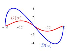
Figure 13: The $D$-terms in the model with $N=1$ profile and $a=0.5$: ${\cal D}(\alpha)$ was obtained using analytic regularization, and $D(\alpha)$ was obtained for $T_{0}=0$ in the model of the previous section.

Our main point is that representing $H(x,\xi)$ as the sum $H_{+}(x,\xi)+H_{D}(x,\xi)$ one can derive the GPD sum rule (71) without using the analyticity assumption. But since our derivation, so to say, works for any $D$-term, it also works for the $D$-term following from the analyticity assumption.

IV.4 Generic sum rule

Finally, let us apply the “DD+D” separation to the generic relation (70).

IV.4.1 “Plus” part

Representing

$$\frac{1}{x-\xi}=\frac{1}{x}+\frac{\xi}{(x-\xi)x}$$ (100)

and using Eqs. (83), (87), we have

$$P\int_{-1}^{1}\frac{H_{+}(x,x)}{x-\xi}\,dx=P\int_{-1}^{1}\xi\,\frac{dx}{x-\xi}\,\int_{\Omega}f(\beta,\alpha)\,\,d\beta\,d\alpha$$

$$\times\biggl{[}\delta(x(1-\alpha)-\beta)-\delta(x(1-\alpha))\biggr{]}$$ (101)

$$=P\int_{\Omega}f(\beta,\alpha)\,\,d\beta\,d\alpha\biggl{[}\frac{\xi}{\beta-\xi(1-\alpha)}+\frac{1}{(1-\alpha)}\biggr{]}\ ,$$

and

$$P\int_{-1}^{1}\frac{H_{+}(x,\xi)}{x-\xi}\,dx=P\int_{-1}^{1}\xi\,\frac{dx}{x-\xi}\,\int_{\Omega}f(\beta,\alpha)\,\,d\beta\,d\alpha$$

$$\times\biggl{[}\delta(x-\beta-\xi\alpha)-\delta(x-\xi\alpha)\biggr{]}$$ (102)

$$=P\int_{\Omega}f(\beta,\alpha)\,\,d\beta\,d\alpha\biggl{[}\frac{\xi}{\beta-\xi(1-\alpha)}+\frac{1}{(1-\alpha)}\biggr{]}\ .$$

Thus, seemingly different delta-functions have converted $1/(x-\xi)$ into identical expressions (cf. Ref. Diehl and Ivanov (2007), where a similar result was obtained for the $F_{D}$ part of the two-DD representation). As a result,

$$P\int_{-1}^{1}\frac{H_{+}(x,x)}{x-\xi}\,dx-P\int_{-1}^{1}\frac{H_{+}(x,\xi)}{x-\xi}\,dx=0\ .$$ (103)

In this case, we deal with the situation when the difference of two integrals vanishes, but each integral does not necessarily vanish.

IV.4.2 “$D$” part

For the integral involving the border function, we have

$$P\int_{-1}^{1}\frac{H_{D}(x,x)}{x-\xi}\,dx=P\int_{-1}^{1}\frac{H_{D}(x,x)}{x}\frac{x}{x-\xi}\,dx$$

$$=P\int_{-1}^{1}dx\,\frac{x}{x-\xi}\,\delta(x)\int_{-1}^{1}\frac{D(\alpha)}{\alpha(1-\alpha)}\,d\alpha=0\ .$$ (104)

In simple words, the starting integrand in (104) vanishes for $x\neq 0$ since then $H_{D}(x,x)=0$, while for $x=0$ it is given by the $x\delta(x)$ distribution which produces zero after integration with a function that is finite for $x=0$, which is the case if $\xi\neq 0$. Comparing this result with Eq. (90), we see that the nonzero value given by the latter cannot be obtained by taking $\xi=0$ in the final result of Eq. (104) above.

The second piece is given by

$$P\int_{-1}^{1}\frac{H_{D}(x,\xi)}{x-\xi}\,dx=P\int_{-1}^{1}\frac{H_{D}(x,\xi)}{x}\,\frac{x}{x-\xi}\,dx$$

$$=P\int_{-1}^{1}\frac{x\,dx}{x-\xi}\,\int_{-1}^{1}\frac{D(\alpha)}{\alpha}\,\delta(x-\xi\alpha)\,d\alpha$$

$$=\int_{-1}^{1}\frac{\xi\alpha}{\xi\alpha-\xi}\frac{D(\alpha)}{\alpha}\,\,d\alpha=-\int_{-1}^{1}\frac{D(\alpha)}{1-\alpha}\,d\alpha\ .$$ (105)

Again, the result above may be obtained by simply using $H_{D}(x,\xi)={\rm sign}(\xi)\,\theta(|x|<|\xi|)D(x/\xi)$ and rescaling $x=\alpha\xi$. Also, though the final result of Eq. (105) does not depend on $\xi$, it does not coincide with the result of the counterpart relation (89).

However, for the difference of the two integrals we obtain

$$P\int_{-1}^{1}\frac{H_{D}(x,x)}{x-\xi}\,dx-P\int_{-1}^{1}\frac{H_{D}(x,\xi)}{x-\xi}\,dx=\int_{-1}^{1}\frac{D(\alpha)}{1-\alpha}\,d\alpha\ ,$$ (106)

the same result as in Eq. (91). Combining the results for the “plus” and $D$-parts gives Eq. (70).

IV.4.3 Some conclusions

Thus, our calculation confirms the generic GPD sum rule (70) derived in Refs. Anikin and Teryaev (2007); Diehl and Ivanov (2007). We were also able to derive the $\xi=0$ sum rule (71) suggested in Ref. Anikin and Teryaev (2007). It should be emphasized that the integrals present in the generic sum rule have a singularity for $x=\xi$, which is inside the region of integration, so the integrals may be taken using the principal value prescription. Since $H(x,0)/x$ and $H(x,x)/x$ are even functions of $x$, the $\xi=0$ sum rule may be written through an integral from 0 to 1, and its $1/x$ singularity is at the end-point of the integration region, which means that the $P$-prescription cannot regulate it. Just because of this fact alone, the sum rule (71) cannot be a straightforward consequence of the generic sum rule (70).

In our derivation, we managed to obtain finite expressions for each term involved. In particular, we established that though $H_{D}(x,x)$ and $H_{D}(x,\xi)$ contributions to the generic sum rule (70) are $\xi$-independent, they do not coincide with their counterparts from the secondary sum rule (71), i.e., the latter cannot be obtained by formally continuing to $\xi=0$ the $\xi$-independent results for each term of the generic GPD sum rule.

In our derivation, we did not make an assumption about analyticity of the Mellin moments of GPDs. We have obtained GPD sum rules as a consequence of the polynomiality of GPDs that follows from Lorentz invariance and is encoded in the DD representation. The analyticity is a much stronger restriction. One may try to find out whether it can be tested experimentally and it is also worth trying to prove it in QCD.

V Summary

In this paper, we discussed some basic aspects of building models for GPDs using the factorized DD Ansatz (FDDA) within the “single-DD” formulation. The main difficulty in the implementation of such a construction is the necessity to deal with projection onto a more singular function $f(\beta)/\beta$ (rather than just onto $f(\beta)$) in the forward limit. This leads to two problems. First, one encounters non-integrable singularities for $\beta=0$ in the integrals producing GPDs in the central region $|x|<|\xi|$. The difficulty is exaggerated by necessity to consider forward distributions $f(\beta)$ that have a singular $\beta^{-a}$ Regge behavior at small $\beta$. Second, if there are no factors suppressing the $\beta\sim 0$ region for the integration line corresponding to $x=\xi$, the combined $1/\beta^{1+a}$ singularity leads to a singular $(x-\xi)^{-a}$ behavior for GPDs in the outer region $x>\xi$ near the border point $x=\xi$. Such a behavior was found in the model of Ref. Szczepaniak et al. (2009).

In our analysis, we found that this model gives the single-DD-type representation for the model GPD, and thus above reasoning is applicable to it. But we argued, that a proper softening of the hadron-quark vertices produces a profile function $h_{N}(\beta,\alpha)$ that results, for $x=\xi$, in the ${\cal O}(\beta^{N})$ suppression factor securing a finite value of the GPD $H(x,\xi)$ at the border point.

However, the profile factor has no impact on the combined $1/\beta^{1+a}$ singularity on the $\beta=0$ line inside the support rhombus, which one faces when calculating GPDs in the $|x|<|\xi|$ region. The advantage of the model of Ref. Szczepaniak et al. (2009) is that it implants the Regge behavior through a subtracted dispersion relation for the hadron-quark scattering amplitude. We found that the subtraction provides the regularization necessary for the calculation of GPDs in the central region, and illustrated the behavior of resulting GPDs in models with $N=1$ and $N=2$ profiles.

We also observed that this model produces a $D$-term contribution, despite the fact that it uses only the forward distribution as an input. This $D$-term contribution appears because the subtraction generated by the dispersion relation differs from the subtraction that converts the original DD into a “plus” distribution $[f(\beta,\alpha)]_{+}$. The latter, by definition, cannot generate a $D$-term. We have shown that the GPD $H_{+}(x,\xi)$ generated by the $[f(\beta,\alpha)]_{+}$ part of the original DD (i.e., GPD $H(x,\xi)$ with the $D$-term contribution $D(x/\xi)$ subtracted) has a remarkable property that the integral of $H_{+}(x,\xi)/x$ over positive values $0\leq x\leq 1$ vanishes. As a result, $H_{+}(x,\xi)$ must be negative in some part of the central region, a feature that is absent in previous FDDA models based on two-DD formulation.

Within the single-DD formalism, it is very natural to separate the relevant DD $f(\beta,\alpha)$ into the “plus” part $[f(\beta,\alpha)]_{+}$ and the $D$-term. We demonstrated that this separation can be used to rederive the GPD sum rule related to the dispersion relation for the real part of the DVCS amplitude, and we also gave a derivation of another sum rule proposed as the $\xi\to 0$ limit of that generic sum rule. Our derivation shows that this “secondary” sum rule is not a straightforward consequence of the generic one. In particular, the principal value prescription used in the generic sum rule needs to be substituted by another prescription, like the “plus” prescription. The “plus” prescription, in fact, is automatically generated by the separation of DDs into the “plus” part and the $D$-term. We also demonstrated that the contributions into the two sum rules generated by the same functions are not in a one-to-one correspondence.

Summarizing, using (intentionally) simplified models, we developed the basic tools that can be used in building realistic GPD models based on the factorized DD Ansatz within the single-DD formalism. Future developments in this direction should include the extension of the presented methods onto the cases with $a>1$ Regge behavior, which would require an extra subtraction in the dispersion relation, and building models for nucleons and other targets with a non-zero spin.