Optimal quasi-free approximation:
reconstructing the spectrum from ground state energies

Abstract

The sequence of ground state energy density at finite size, $e_{L}$, provides much more information than usually believed. Having at disposal $e_{L}$ for short lattice sizes, we show how to re-construct an approximate quasi-particle dispersion for any interacting model. The accuracy of this method relies on the best possible quasi-free approximation to the model, consistent with the observed values of the energy $e_{L}$. We also provide a simple criterion to assess whether such a quasi-free approximation is valid. As a side effect, our method is able to assess whether the nature of the quasi-particles is fermionic or bosonic together with the effective boundary conditions of the model. When applied to the spin-1/2 Heisenberg model, the method produces a band of Fermi quasi-particles very close to the exact one of des Cloizeaux and Pearson. The method is further tested on a spin-1/2 Heisenberg model with explicit dimerization and on a spin-1 chain with single ion anisotropy. A connection with the Riemann Hypothesis is also pointed out.

I introduction

The way finite-size, thermodynamic, averages approach their infinite size limit, encodes a wealth of precious information. Take for example a quantum system at zero temperature, and consider the ground state energy density at finite size $e_{L}$, $L$ being the linear size of the system. A piece of common knowledge in condensed matter theory –not yet a theorem though– asserts that, for a massive (i.e. gapped) system with translation and Left-Right invariance, the approach to the thermodynamic limit is exponentially fast, that is $e_{L}\rightarrow e_{\infty}+O\left(e^{-L/\xi_{E}}\right)$ where the decay rate $\xi_{E}$ is somehow related to the correlation length of the system $\xi_{C}$. On the contrary, in a critical theory, the correlation length is formally infinity and the approach is expected to be of algebraic type. Moreover for conformal field theories (CFT) in $\left(1+1\right)$ dimensions and periodic boundary conditions, it is known that $e_{L}=e_{\infty}-\left(\pi/6\right)cv/L^{2}+o\left(L^{-2}\right)$ Blöte et al. (1986); Affleck (1986) where $v$ is the speed of elementary excitations and $c$ is the all-important central charge of the CFT. From these argument it seems clear that it should be possible, by simply looking at the sequence $e_{L}$, to discern whether the theory is critical or gapped. In fact, even though the standard method to locate critical point is that of looking at the gap closure, recent studies have shown that accurate methods to locate critical points are available, which resort solely to the computation of ground state averages such as the total energy and the perturbation Roncaglia et al. (2008).

In this article we will show that the sequence $e_{L}$ provides in fact much more information. We will show that, by knowing $e_{L}$ for few short sizes $L$, it is possible to reconstruct approximately the one particle dispersion of the theory. Perhaps most importantly, analyzing the sequence $e_{L}$, one is able to assess whether the quasi-particles of the theory have fermionic or bosonic character together with the effective boundary conditions of the model.

If the Hamiltonian $H$ under consideration admits a quasi-free representation (i.e. the Hamiltonian can be expressed as a quadratic form in Fermi or Bose operators), our algorithm produces a one-particle dispersion rapidly converging to the exact one, as we increase the number of available ground state energies. In practice having 10 energy data produces a result indistinguishable from the exact one.

Conversely, if $H$ is truly interacting, we obtain an approximate one-particle dispersion corresponding to a quasi-free model $\tilde{H}$. The Hamiltonian $\tilde{H}$ so obtained, is the simplest quasi-free model whose ground state energies are the same as those observed for $H$.

For quasi-free models the mathematical problem is related to that of reconstructing a function given some of its partial Riemann sums. As we will show, assessing the convergence speed of this method is a problem connected to the Riemann hypothesis. Let us then begin by considering the problem of convergence of Riemann sums.

II Convergence of Riemann sums

As we will show in greater detail in section IV, the finite-size, ground state energy of any, translation invariant, quasi-free system, consisting either of bosons or of fermions, is related to a Riemann sum of the following form

$$S_{L}\left(f\right)=\frac{1}{L}\sum_{n=0}^{L-1}f\left(\frac{2\pi n+\vartheta}{L}\right).$$ (1)

Here $L$ is precisely the size of the one-dimensional lattice and $f$ a suitable function related to the one-particle dispersion. The points $k_{n}=\left(2\pi n+\vartheta\right)/L$ are quasimomenta which define the Brillouin zone $BZ=[0,2\pi)$ for finite $L$, and the angle $\vartheta\in\left[0,\pi\right]$ defines general, twisted boundary conditions (TBC). In terms of canonical operator (either bosons or fermions) $c_{x}$, TBC means $c_{x+L}=e^{i\vartheta}c_{x}$. The angle $\vartheta$ allows to interpolate continuously between periodic (PBC) $\vartheta=0$ and antiperiodic (ABC) $\vartheta=\pi$ boundary conditions.

Since the function $f$ is defined on $[0,2\pi)$ it is useful to write it as a Fourier series:

$$f\left(k\right)=\sum_{n=-\infty}^{\infty}c_{n}e^{ink},\quad c_{n}=\frac{1}{2\pi}\int_{0}^{2\pi}e^{-i\xi n}f\left(\xi\right)d\xi.$$ (2)

In order to obtain an explicit formula for Eq. (1) we would like to apply the operator $S_{L}$ to the exponentials appearing in Eq. (2) (i.e. swap $S_{L}$ with the sum). To this end we need to assume some regularity in the convergence of the sum (2) such as absolute convergence. Necessary conditions for absolute convergence of Eq. (2) are known; for instance it is enough to have $f$, $\alpha$-Hölder continuous with $\alpha>1/2$, or $f$ of bounded variation and $\alpha>0$. On physical grounds we can assume such conditions will be satisfied, they are indeed satisfied in all examples encountered. Now, assuming absolute convergence of the series in Eq. (2) we can apply the operator $S_{L}$ to the exponentials obtaining

$$S_{L}\left(e^{ink}\right)=\frac{e^{in\vartheta/L}}{L}\frac{\left(1-e^{i2\pi n}\right)}{\left(1-e^{i2\pi n/L}\right)}.$$ (3)

This equation is zero for all natural $n$ not multiple of $L$, whereas for $n=lL$ with $l\in\mathbb{Z}$, equals $e^{il\vartheta}$. Therefore we can compactly write $S_{L}\left(e^{ink}\right)=\sum_{l=-\infty}^{\infty}e^{il\vartheta}\delta_{n,lL}$. Combining this result with Eq. (2) we obtain

$$S_{L}\left(f\right)-c_{0} = \sum_{l=1}^{\infty}e^{il\vartheta}c_{lL}+e^{-il\vartheta}c_{-lL}$$ (4)

$$= 2\mathrm{Re}\sum_{l=1}^{\infty}e^{il\vartheta}c_{lL},$$ (5)

where the last line follows from the reality of $f$.

Assume now that the function $f$ is $2\pi$-periodic and analytic. Then there exist a strip in the complex plane $\mathcal{A}=[0,2\pi]\times[-\sigma,\sigma]$ such that $f$ can be extended to an analytic, bounded function on $\mathcal{A}$. In this case Fourier coefficients can be computed in the complex plane $z$, integrating on a horizontal line shifted by an imaginary amount $-i\sigma$. The vertical contributions cancel each other because of periodicity and we can write

$$c_{n}=\frac{1}{2\pi}\int_{0-i\sigma}^{2\pi-i\sigma}e^{-inz}f\left(z\right)dz.$$ (6)

At this point the geometric series of the exponential converges absolutely and we obtain

$$S_{L}\left(f\right)-c_{0}=\mathrm{Re}\left[\frac{1}{\pi}\int_{0-i\sigma}^{2\pi-i\sigma}\frac{f\left(z\right)dz}{e^{i\left(zL-\vartheta\right)}-1}\right].$$ (7)

This formula is remarkable; it allows to show that, for periodic analytic functions, the convergence of partial Riemann sum to the limiting integral, is at least exponentially fast in the size $L$. More precisely, since $1/\left|e^{i\left(zL-\vartheta\right)}-1\right|\leq 1/\left(e^{\sigma L}-1\right)$ for all $z$ in $\mathcal{A}$ and $\vartheta=0,\pi$, using (7) we obtain

$$\left|S_{L}\left(f\right)-c_{0}\right|\leq 2\max_{z\in\mathcal{A}}\left|f\left(z\right)\right|\frac{1}{e^{\sigma L}-1}.$$ (8)

This shows that, for analytic periodic functions $f$, the partial sum $S_{L}\left(f\right)$ converges at least exponentially fast in $L$ to its limiting value. Moreover Eq. (8) gives a simple way to compute the decay rate. All we have to do is take $\sigma$ as large as possible, i.e. find the largest strip $\mathcal{A}$ where the function is analytic. This amounts to look for the singularity of $f$ closest to the real axis, let it be $z_{0}$. The imaginary part $\xi_{E}^{-1}=\mathrm{Im}\left(z_{0}\right)=\max\sigma$ gives the decay rate and from Eq. (8) we obtain $\left|S_{L}\left(f\right)-c_{0}\right|\leq O\left(e^{-L/\xi_{E}}\right)$.

As we will discuss in greater detail in section IV, for quasi-free systems (that is, Hamiltonians quadratic in Fermi or Bose canonical operators), the ground state energy is exactly given by an expression of the form of Eq. (1) where the function $f$ is proportional to the one-particle dispersion. The result above shows that if the one particle band is a positive, analytic, periodic function, the ground state energy density approaches its limit exponentially fast. The positivity requirement on the band implies that the system has a gap. So we reach the conclusion that for gapped theories with analytic dispersion, the energy density decays at least exponentailly with the size –at least for the case of quasi-free systems. Since, from scaling hypothesis, the correlation length is the only length-scale of the system, we expect the decay rate $\xi_{E}$ to be related to the correlation length.

Equation (7) cannot be used when the function is not analytic on $\left[0,2\pi\right]$, in this case the difference $S_{L}\left(f\right)-c_{0}$ can be estimated using Euler-Maclaurin formula. In any case, for critical theories where the dispersion vanishes linearly as $\omega\left(k\right)\sim v\left|k-k_{F}\right|^{z}$ (here $z$ is the dynamical exponent and $k_{F}$ the Fermi momentum) scaling theory predicts an algebraic approach of the form $S_{L}\left(\omega\right)-c_{0}=O\left(L^{-1-z}\right)$ (see e.g. Barber (1983)). An example in this class is given by the function $\left|\cos\left(k\right)\right|$, which is continuous but not differentiable. An explicit calculation shows in fact $S_{L}\left(\left|\cos\left(k\right)\right|\right)-2/\pi=O\left(L^{-2}\right)$ consistent with $z=1$. To complete the scenario we should mention another possibility which gives rise to an algebraic approach to the thermodynamic limit. Namely the function itself might have a jump at some point as it happens, for instance, to the function $k$. In fact $0$ and $2\pi$ should be identified in the Brillouin zone and this function has a jump of value $2\pi$. In fact in this case we have $S_{L}\left(k\right)=\pi-\pi/L$. This situation typically takes place in physical systems when Left-Right symmetry is explicitly broken.

Our aim here is to reconstruct $f$ given $S_{L}\left(f\right)$, that is, we would like somehow to invert Eq. (7). To this end it is better to do a step back.

III Solution of the inverse problem

Even in the most favorable case, we can hope to have at disposal only a finite number of partial sum $S_{m}\left(f\right)$, say the first $L$ (obtained, for instance by Lanczos diagonalization, see sec. IV). This means we can only reconstruct $f$ through $L$ coefficients. A sensible choice, and in some sense the best one, is that of reconstructing the first $L$ Fourier coefficients of $f$.

In the rest of the article we will concentrate on the physically most important periodic and anti-periodic BC’s for which $\vartheta=0,\,\pi$. In these cases the partial Riemann sums are identically zero for $f$ odd, i.e. $S_{L}^{\left(\vartheta\right)}\left(f\right)=0$ for $f\left(k\right)=-f\left(-k\right)[=-f\left(2\pi-k\right)]$. Clearly, having at disposal the numbers $S_{L}^{\left(\vartheta\right)}\left(f\right)$ we can only hope to re-construct the even part of $f$. Fortunately, on physical grounds we can suppose that the function $f$ will indeed be even in $k$. This corresponds to Left-Right symmetry on top of translational symmetry and it is a reasonable assumptions valid in most physical situations. A breaking of Left-Right symmetry happens, for instance, when inserting a periodic spin chain in a magnetic field of flux $\vartheta\hbar c/e$ Byers and Yang (1961). Such a problem can usually be reformulated into the same problem without magnetic field and TBC specified by the angle $\vartheta$. All in all considering $\vartheta=0,\,\pi$ is consistent with assuming $f$ even.

Assume then that the function $f$ is even so that its Fourier series has only cosine coefficients. For PBC and ABC, $e^{i\vartheta}$ is real and, defining $R_{L}\left(f\right)=S_{L}\left(f\right)-c_{0}$, we can re-write Eq. (4) in matrix notation as $\boldsymbol{R}=\mathcal{G}\boldsymbol{a}$, where boldface indicates column vector and the matrix $\mathcal{G}$ has components given by

$$\mathcal{G}_{M,m}=\sum_{l=1}^{\infty}e^{i\vartheta l}\delta_{m,lM}\,.$$ (9)

The components of the vector $\boldsymbol{a}$ are the cosine Fourier coefficients

$$a_{n}=2\mathrm{Re}c_{n}=\frac{1}{\pi}\int_{0}^{2\pi}\cos\left(\xi n\right)f\left(\xi\right)d\xi.$$ (10)

Note that both $\mathcal{G}$ and $\boldsymbol{a}$ are real. To solve for the first $L$ Fourier coefficients we truncate the equation to the first $L$ terms to obtain $\boldsymbol{R}^{\left(L\right)}=\mathcal{G}^{\left(L\right)}\boldsymbol{a}^{\left(L\right)}$, where $\boldsymbol{R}^{\left(L\right)}=\left(R_{1},R_{2},\ldots,R_{L}\right)^{\top}$, $\boldsymbol{a}^{\left(L\right)}=\left(a_{1},a_{2},\ldots,a_{L}\right)^{\top}$ and $\mathcal{G}^{\left(L\right)}$ is the $L\times L$ matrix with entries given by Eq. (9) for $M,m\leq L$. For example, for $L=6$ , the matrix $\mathcal{G}^{\left(6\right)}$ reads

$$\mathcal{G}^{\left(L=6\right)}=\left(\begin{array}[]{cccccc}q&q^{2}&q^{3}&q^{4}&q^{5}&q^{6}\\ 0&q&0&q^{2}&0&q^{3}\\ 0&0&q&0&0&q^{2}\\ 0&0&0&q&0&0\\ 0&0&0&0&q&0\\ 0&0&0&0&0&q\end{array}\right).$$ (11)

with $q=e^{i\vartheta}=\pm 1$. Since $\det\left(\mathcal{G}^{\left(L\right)}\right)=q^{L}\neq 0$ the matrix is invertible and defines a bijection. It is then possible to obtain the first $L$ Fourier components approximately via $\boldsymbol{a}^{\left(L\right)}=\left[\mathcal{G}^{\left(L\right)}\right]^{-1}\boldsymbol{R}^{\left(L\right)}$. One can show that the inverse matrix has the same structure as $\mathcal{G}^{\left(L\right)}$ in the sense that $\left[\mathcal{G}^{\left(L\right)}\right]^{-1}$ has non zero entries in the same places as $\mathcal{G}^{\left(L\right)}$. More precisely $\left(\left[\mathcal{G}^{\left(L\right)}\right]^{-1}\right)_{i,j}=b\left(j/i\right)$ if $j/i\in\mathbb{N}$ and zero otherwise, for some numeric function $b\left(n\right)$. Using a similar notation as before, this means

$$\left(\left[\mathcal{G}^{\left(L\right)}\right]^{-1}\right)_{i,j}=\sum_{l=1}^{\left[L/i\right]}b\left(l\right)\delta_{j,li}\,.$$ (12)

Imposing $\left[\mathcal{G}^{\left(L\right)}\right]^{-1}\mathcal{G}^{\left(L\right)}=\leavevmode{\rm 1\mkern-4.8muI}$ we get the equation defining $b\left(m\right)$:

$$\sum_{\stackrel{{\scriptstyle m=1}}{{j/m\in\mathbb{N}}}}^{j}e^{i\vartheta j/m}b\left(m\right)=\delta_{1,j}\,.$$ (13)

The above sum extends over all positive divisors of $m$ and is usually denoted by $\sum_{j|m}$ (read $j$ divides $m$) in the mathematical literature. Equation (13) provides a recursive solution for $b\left(m\right)$: $b\left(1\right)=e^{-i\vartheta}$ while $b\left(j\right)=-e^{-i\vartheta}\sum_{\stackrel{{\scriptstyle m=1}}{{j/m\in\mathbb{N}}}}^{j-1}e^{i\vartheta j/m}b\left(m\right)$ for $j\geq 2$. Since Eq. (13) is independent of $L$, it implies that $\left[\mathcal{G}^{\left(L\right)}\right]^{-1}$ is the first $L\times L$ sub-matrix on the diagonal of $\left[\mathcal{G}^{\left(M\right)}\right]^{-1}$ for any $L<M$. In particular any $\left[\mathcal{G}^{\left(L\right)}\right]^{-1}$ can be obtained from the infinite case $\mathcal{G}^{-1}$ and its entries do not depend on $L$. Now the inverse formula $\boldsymbol{a}^{\left(L\right)}=\left[\mathcal{G}^{\left(L\right)}\right]^{-1}\boldsymbol{R}^{\left(L\right)}$, in components reads

$$a_{k}^{\left(L\right)}\left(f\right)=\sum_{n=1}^{\left[L/k\right]}b\left(n\right)R_{nk}\left(f\right),$$ (14)

where we explicitly indicated the dependence on the function $f$. The superscript $\left(L\right)$ indicates that the Fourier coefficients are obtained only approximately, but with increasing precision the larger the $L$. The result of the reconstruction is optimal in the sense that it produces the unique trigonometric polynomial of degree $L$ consistent with the “observed” data $S_{L}$. In the limit $L\to\infty$ – that means we know $R_{L}\left(f\right)$ for arbitrary $L$ – we can reproduce the function exactly and $a_{k}^{\left(L\right)}\left(f\right)\to a_{k}\left(f\right)$. To be mathematically precise, this last assertion is satisfied provided $f$ is not too pathological. On physical ground we can safely discard such pathological cases. On the contrary Eq. (14) can be used to obtain information on the function $f$. For what discussed in the previous section, the only potentially dangerous case is that of a critical point. Since physically we will identify $R_{L}\left(f\right)$ with the finite size energy density, scaling arguments predict that, at a critical point, $R_{L}\left(f\right)\sim L^{-1-z}$ where $z$ is the dynamical critical exponent. Now one can use Eq. (14) to obtain $a_{k}\sim k^{-1-z}$ which gives rise to a function with absolutely convergent Fourier series.

The PBC case $\vartheta=0$ provides some interesting connections to number theory. In this case in fact Eq. (13) becomes the equation defining the Möbius function $\mu\left(m\right)$ , i.e. Eq. (13) is solved by $b\left(n\right)=\mu\left(n\right)$. Note also that, for $q=1$, $\mathcal{G}^{\left(L\right)}$ is very similar to the Redheffer matrix $\mathcal{R}^{\left(L\right)}$ known in number theory Redheffer (1977). The matrix $\mathcal{R}^{\left(L\right)}$ is the same as $\mathcal{G}^{\left(L\right)}$ except for the first column which is made of one. The importance of the Redheffer matrix originates from the fact the $\det\mathcal{R}^{\left(L\right)}=M(L):=\sum_{n=1}^{L}\mu\left(n\right)$ where $M\left(L\right)$ is the Mertens function. The statement $M\left(L\right)=O\left(L^{1/2+\epsilon}\right)$ is equivalent to the Riemann hypothesis.

III.1 Convergence rate

Since we are assuming the function we seek is even, Eq. (2) becomes $f\left(k\right)=c_{0}+\sum_{n=1}^{\infty}a_{n}\cos\left(nk\right)$. If we have access to the partial Riemann sums up to $L$ (and the limiting value $c_{0}$), we can reconstruct an approximate function given by

$$f_{L}\left(k\right)=c_{0}+\sum_{n=1}^{L}a_{n}^{\left(L\right)}\cos\left(nk\right),$$ (15)

with $a_{n}^{\left(L\right)}$ given by equation (14). We can now ask how fast this method allows to reproduce the function $f$. The question of convergence of Fourier series has engaged mathematicians for centuries. The problem of convergence of the series (15) is likely to be more complex. Here we will content to give some arguments for the physically important cases related to massive and critical theory.

To be specific we will consider PBC. We can safely assume $f$ to be square summable. The reconstructed function $f_{L}$ is obviously also square summable, being a trigonometric polynomial. The $L^{2}\left(\left[0,2\pi\right]\right)$ square distance reads

$$\left\|f_{L}-f\right\|_{2}^{2}=\pi\sum_{n=1}^{L}\left(a_{n}^{\left(L\right)}-a_{n}\right)^{2}+\pi\sum_{n=L+1}^{\infty}a_{n}^{2}.$$ (16)

Consider first the case where $f$ is periodic and analytic in $\left[0,2\pi\right]$. In this case a saddle point argument shows that the Fourier coefficients decay exponentially $c_{n}=O\left(e^{-n/\xi_{F}}\right)$. Moreover the correlation length $\xi_{F}$ is precisely the same as that appearing in Sec. II: $\xi_{F}=\xi_{E}$. Hence the second sum in Eq. (16) is of the order of $e^{-2L/\xi_{E}}$. To estimate the first sum consider

$$a_{n}^{\left(L\right)}-a_{n}=\sum_{m=\left[L/n\right]+1}^{\infty}b\left(m\right)R_{nm}\,.$$ (17)

For what discussed in Sec. II, $R_{m}=O\left(e^{-m/\xi_{E}}\right)$. For PBC $\left|b\left(m\right)\right|=\left|\mu\left(m\right)\right|\leq 1$ so that $\left|a_{n}^{\left(L\right)}-a_{n}\right|\leq\sum_{m=\left[L/n\right]+1}^{\infty}\left|R_{nm}\right|$. This implies that, for sufficiently large $L$, $\left|a_{n}^{\left(L\right)}-a_{n}\right|\leq O\left(e^{-L/\xi_{E}}\right)$, so that, in turn, the first sum in Eq. (16) is bounded by $Le^{-2L/\xi_{E}}$. All in all, if $f$ is periodic and analytic in $\left[0,2\pi\right]$, $f_{L}$ is exponentially close to $f$, in sense that $\left\|f_{L}-f\right\|_{2}^{2}\leq O\left(Le^{-2L/\xi_{E}}\right)$.

Consider now the critical case. From a physical point of view, a critical theory with dynamical exponent $z$ corresponds to excitations vanishing as $f\left(k\right)\sim k^{z}$, with $z>0$. A scaling argument now implies that the Fourier coefficients of such a function scale as $c_{n}\sim n^{-1-z}$. More precisely assume that, for large enough $n$ $\left|c_{n}\right|\leq An^{-1-z}$ with $A$ positive constant. Let us first consider the second sum in Eq. (16)

$$\left|\sum_{n=L+1}^{\infty}a_{n}^{2}\right| \leq A^{2}\sum_{n=L+1}^{\infty}n^{-2-2z}\,.$$ (18)

We can use the asymptotic behavior $\sum_{n=M}^{\infty}n^{-\alpha}\sim\left(\alpha-1\right)^{-1}/M^{\alpha-1}$ to estimate $\left|\sum_{n=L+1}^{\infty}a_{n}^{2}\right|\lesssim A^{2}\left(1+2z\right)^{-1}/L^{1+2z}$. To obtain the behavior of the first sum in Eq. (16) we first look at Eq. (4) and obtain, for $L$ large enough $\left|R_{L}\right|\leq 2AL^{-1-z}\zeta\left(1+z\right)$. Then

$$\left|a_{n}^{\left(L\right)}-a_{n}\right|\leq\frac{2A\zeta\left(1+z\right)}{n^{1+z}}\sum_{m=\left[L/n\right]+1}^{\infty}\frac{1}{m^{1+z}}.$$ (19)

Using the same estimate as before we obtain $\left|a_{n}^{\left(L\right)}-a_{n}\right|\lesssim 2A\zeta\left(1+z\right)z^{-1}/(nL^{z})$ and so $\sum_{n=1}^{L}\left|a_{n}^{\left(L\right)}-a_{n}\right|^{2}\lesssim A^{\prime}/(L^{2z})\sum_{n=1}^{L}n^{-2}\lesssim A^{\prime\prime}/(L^{2z})$. So it seems that the convergence rate of $\left\|f_{L}-f\right\|_{2}^{2}$ is of the order of $L^{-2z}.$ Here we would like to conjecture that the first sum in Eq. (16) actually introduces corrections that are roughly of the same order as the second, i.e. $\left\|f_{L}-f\right\|_{2}^{2}\sim L^{-1-2z}$. The argument is based on the Riemann hypothesis. Consider again $a_{n}^{L}-a_{n}$ in the PBC case. For $L$ sufficiently large we have

$$a_{n}^{L}-a_{n}\sim n^{-1-\zeta}\sum_{m=\left[L/n\right]+1}^{\infty}\mu\left(m\right)m^{-1-\zeta}.$$ (20)

An equivalent statement to the Riemann hypothesis is that the Mertens function $M\left(x\right):=\sum_{m=1}^{x}\mu\left(m\right)$ satisfies $M\left(x\right)=O\left(x^{1/2+\epsilon}\right)$ for any positive $\epsilon$. Using partial summation we can estimate $\sum_{m=M}^{\infty}\mu\left(m\right)m^{-\alpha}=O\left(M^{1/2-\alpha+\epsilon}\right)$ for $\alpha>1/2$. Plugging this estimate in Eq. (20) we obtain

$$a_{n}^{L}-a_{n}\sim\frac{L^{-1/2-z+\epsilon}}{n^{1/2+\epsilon}}\,,$$ (21)

from which roughly $\sum_{n=1}^{L}\left(a_{n}^{L}-a_{n}\right)^{2}\sim L^{-1-2z+\epsilon}$.

To summarize, in the case of analytic functions, relevant to massive Left-Right symmetric models, we expect exponential convergence speed with rate given by the correlation length. For critical theories with dynamical exponent $z$, we expect an algebraic convergence speed. Resorting to the Riemann Hypothesis we conjecture the convergence speed to be of the order of $L^{-1-2z+\epsilon}$.

To visualize better how fast the method works, consider an example taken from physics where the function to reconstruct is given by

$$f\left(k\right)=J\sqrt{\sin\left(k/2\right)^{2}+m^{2}}.$$ (22)

Such a function is a periodic generalization of a relativistic dispersion and it describes, exactly or approximately, the one-particle dispersion of many one dimensional systems. When $m\neq 0$ the function is analytic in $\left[0,2\pi\right]$ and the convergence is exponentially fast. The case $m=0$ can serve to model critical theories with dynamical exponent $z=1$. In this case the convergence in the $L^{2}$-norm, is algebraic and we just conjectured that the rate is of the order of $L^{-3}$. This behavior is confirmed in figure 1 which shows that, for the massive case, $\ln\left(\left\|f_{L}-f\right\|_{2}^{2}\right)$ is approximately linear with $L$, while for $m=0$ we have roughly $\ln\left(\left\|f_{L}-f\right\|_{2}^{2}\right)\leq-3\ln L+\mathrm{const.}$.

The result of the reconstruction for the function in Eq. (22) is instead shown in figure 2 for different masses $m$, using PBC and as little as the first ten Riemann sums. Results for ABC are very similar. It is notable the very good agreement even in the massless case.

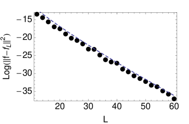
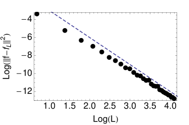
Figure 1: Convergence speed in the $L^{2}\left(\left[0,2\pi\right]\right)$ norm for the function $f\left(k\right)=\sqrt{\sin\left(k/2\right)^{2}+m^{2}}$. The reconstructed function $f_{L}\left(k\right)$ is given by Eqns. (15) and (14) and the $L^{2}\left(\left[0,2\pi\right]\right)$ distance $\left\|f-f_{L}\right\|_{2}^{2}$ is then evaluated for various $L$. Top (bottom) picture refers to massive $m\neq 0$ (massless $m=0$) case. In the massive case the approach expected is of exponential type. The dashed line is given by $\mathrm{const.}\times L^{-3}e^{-2L/\xi_{E}}$, with $\xi_{E}^{-1}=2\mathrm{arcsinh}\left(m\right)$ which can be obtained estimating the Fourier coefficients of $f\left(k\right)$ with a saddle point argument. In the masless case the approach is expected to be of the form $1/L^{3+\epsilon}$ (see main text). The dashed line in the lower panel gives the $L^{-3}$ behavior. The method is tested for PBC, and the mass in the top panel is $m=0.1$.

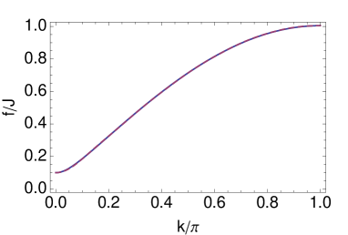
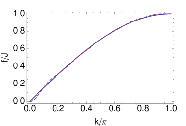
Figure 2: Results of the reconstruction for a prototypical function $f\left(k\right)=J\sqrt{\sin\left(k/2\right)^{2}+m^{2}}$, using as little as ten Riemann sums. Upper panel refers to $m=0.1$ while lower panel to $m=0$. Continuous line is the exact function, while the dashed line is the reconstructed function $f_{L}\left(k\right)$ using PBC. Since the functions are even only half of the Brillouin zone is shown. Note that for $m=0.1$, $f_{L}\left(k\right)$ is indistinguishable from the exact function at this scale. Results for ABC produce very similar plots.

IV Method and applications

The methods discussed so far are readily applicable to translation invariant quasi-free systems consisting either of fermions or bosons. By quasi-free systems we mean here Hamiltonians that can be expressed as quadratic forms in Bose or Fermi operators. In such cases in fact the ground state energy is precisely given by a partial Riemann sum. For example, in the notation of Lieb et al. (1961) a quasi-free fermionic model has the form $H=\sum_{ij}c_{i}^{\dagger}A_{i,j}c_{j}+1/2\left(c_{i}^{\dagger}B_{i,j}c_{j}^{\dagger}+\mathrm{h.c.}\right)$. Diagonalization brings it to $H=\sum_{k}\omega_{k}\eta_{k}^{\dagger}\eta_{k}+\Gamma$, where the band $\omega_{k}$ can be chosen positive and the constant $\Gamma$ is given by $2\Gamma=\mathrm{tr}A-\sum_{k}\omega_{k}$. For translation invariant systems, with PBC or ABC, the label $k$ is a (quasi-) momentum quantized according to $k=\left(2\pi n+\vartheta\right)/L$, $n=0,1,\ldots,L-1$. Defining the “filling fraction” $\nu=1-\mathrm{tr}\left(A\right)/\sum_{k}\omega_{k}$ the Hamiltonian takes the form

$$H=\sum_{k}\omega_{k}\left[\eta_{k}^{\dagger}\eta_{k}-\frac{\nu}{2}\right].$$ (23)

If the model consists of $n$ species of non-interacting colors, i.e. $c_{i}\rightarrow c_{i,\alpha}$, $\alpha=1,\ldots,n$, simply replace $\nu\rightarrow n\nu$. All the methods presented so far can now be applied considering that the ground state energy density of Hamiltonian (23) is precisely given by $e_{L}=E_{L}/L=-\left(\nu/2\right)\sum_{k}\omega_{k}$. Now the point is that in many physically interesting situations the “filling fraction” is known in advance. In fact in absence of (magnetic or electric) fields generally $\nu=1$ (or $\nu=n$ for $n$ non-interacting species) since $\mathrm{tr}A=0$. This means that the $\nu$ in Eq. (23) is independent of $L$, and the ground state energy density is precisely given by a Riemann sum: $e_{L}=-\left(\nu/2\right)S_{L}\left(\omega_{k}\right)$. Similar considerations hold for bosonic quadratic theory with the important difference that now $e_{L}=+\left(\nu/2\right)S_{L}\left(\omega_{k}\right)$, due to the commutation relation.

We can now argue that any interacting model admits some sort of quasi-free approximation. At this level of approximation, the Hamiltonian is quadratic and we can apply all the reasoning presented above. Our method gives a way to obtain a one particle dispersion knowing the ground state energy for some lattice sizes. The dispersion obtained is optimal in the sense that it is the unique trigonometric polynomial of degree $M$ (where $M$ is the number of energy data) consistent with the observed values of the energy. This method bears some similarity with the Hartree-Fock method largely used for ab-initio calculation of molecular systems. The Hartree-Fock method, for a given size $L$, gives the optimal quasi-free state that minimizes the energy. The method proposed here instead, taking $M$ ground state energies as input, gives an optimal quasi-free system (identified with its one-particle dispersion), in the sense that its ground state energies are precisely the $M$ observed value.

To specify completely the problem one has to assume the character of the quasi-free approximation, i.e. whether the model consists of Bosons or Fermions together with the effective boundary conditions. In practice we have to chose if the ground state energy densities are given by $e_{L}=\epsilon\left(\nu/2\right)S_{L}\left(\omega_{k}\right)$ with $\epsilon=\pm 1$ and moments specified by $\vartheta=0,\pi$ (PBC or ABC). This choice can be straightforward if the model under consideration consists of Bosons or Fermions, but in case of spin models, the character of the effective, quasi-free model is less clear. According to the choices $\epsilon=\pm 1$ and $\vartheta=0,\pi$ we have therefore 4 possibilities. However the requirement that the reconstructed band must be positive fixes in practice only two combinations. This is an important result on its own: simply looking at the sequence of ground state energies, one is able to assess whether quasi-particles are Fermions or Bosons with ABC or PBC.

As for any approximation method, it would be derisable to have a simple criterion to assess whether a quasi-free approximation is feasible in the first place. Such a criterion can be given. In fact for exactly quasi free models, the ground state state energies satisfy

$$E_{2L}^{\left(0\right)}=E_{L}^{\left(0\right)}+E_{L}^{\left(\pi\right)},$$ (24)

where the superscript $\left(0\right),\,\left(\pi\right)$ refers to PBC, ABC respectively. So, having finite-size energies for PBC and ABC, we can simply verify the possibility of an effective quasi-free description by checking how well Eq. (24) is satisfied.

For what we have said in section III.1, the procedure of reconstructing a function given its $M$ partial Riemann sums, rapidly converges upon increasing $M$ even in the the critical case (the worst scenario), so that one can effectively limit oneself to short lattice sizes.

For the reader’s sake, let us sketch here the relevant steps of the algorithm:

• Obtain a set of $M$ ground state energies of the system by exact diagonalization of short lattices, say sizes up to $L=10-20$. If both PBC and ABC energies are available one can check the feasibility of a quasi-free approximation by checking how well Eq. (24) is satisfied.

• Assume effective PBC/ABC and Bosons/Fermions which correspond to assume for the ground state energy density $e_{L}=\epsilon\left(\nu/2\right)S_{L}\left(\omega_{k}\right)$ with $\epsilon=\pm 1$ and moments specified by $\vartheta=0,\pi$. An approximate dispersion is then given by Eq. (15) with $f\left(k\right)=\epsilon\left(\nu/2\right)\omega_{k}$ and coefficients specified by Eq. (14). The requirement $\omega\left(k\right)\geq 0$ will fix two cases out of the four possibilities.

• One should also fix the filling fraction $\nu$. If this can be simple when the model is originally given in terms of Bosons or Fermions, in general one must be guided by physical intuition. Referring to the example that will be discussed in the following sections, it is natural to expect $\nu=1$ for the pure spin-1/2 Heisenberg model, a triplet of excitations for its dimerized version ($\nu=3$) and a doublet ($\nu=2$) of excitations for the spin-1 $\lambda-D$ model in the large-$D$ phase.

Let us now illustrate how the method works on the hand of a few concrete, yet prototypical examples.

IV.1 Spin 1/2 Heisenberg model

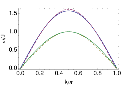
Figure 3: (Color online) Results of our procedures for the spin-1/2 Heisenberg model. The continuous upper curve (blue) is the exact dispersion $\omega\left(k\right)=$$\left(\pi/2\right)J\left|\sin\left(k\right)\right|$, while the continuous lower curve (green) is the result of spin-wave approximation $\omega_{SW}\left(k\right)=J\left|\sin\left(k\right)\right|$. Using only finite size energies up to $L=24$ we obtained upper and lower dashed curve. The lower curve is obtained assuming a bosonic dispersion with effective PBC and can be identified with the spin-wave approximation. The upper dashed curve assumes a dispersion with fermionic character and effective ABC. The very good agreement with the exact result tells us that there exist a quadratic Hamiltonian approximating Heisenberg one very precisely.

Take the Heisenberg antiferromagnetic ($J>0$) chain:

$$H=J\sum_{i=1}^{L}\mathbf{S}_{i}\cdot\mathbf{S}_{i+1}\,.$$ (25)

$\mathbf{S}_{i}$ are spin-1/2 operators at site $i$ and PBC ($\mathbf{S}_{L+1}=\mathbf{S}_{1}$) are used. From the exact solution we know that the infinite size ground state energy is $e_{\infty}/J=1/4-\ln 2$ Hultén (1938), whereas the quasi-particle dispersion is given by $\omega\left(k\right)=\left(\pi/2\right)J\left|\sin\left(k\right)\right|$ des Cloizeaux and Pearson (1962). When we have to evaluate the energy at finite size we immediately face a problem. When $L$ is even the ground state belongs to the total spin $S=0$ sector and is unique Lieb and Mattis (1962). This is the kind of ground state we “expect” from this model. On the contrary, for $L$ odd there are two degenerate spin-1/2 ground states. The ground state energies for $L$ odd have a completely different character and our intuition suggests us to discard them. As a consequence we have access only to $e_{L}$ for even $L$. However, from the exact solution we know that the dispersion is periodic with period halved i.e. $\pi$. Hence it has only even Fourier (cosine) coefficients. From Eq. (14) we see that with even-size energies we can re-construct even Fourier coefficients. In this case the two facts are consistent: $e_{L}$ only for $L$ even $\leftrightarrow$ even Fourier coefficients. The procedure is as follows. First, we diagonalize exactly Hamiltonian (25) with say a Lanczos algorithm. In few minutes of a small laptop computer, we obtained ground state energies for lattices of even size up to $L=24$ . Separately we estimate the infinite size ground state energy which in this case is $e_{\infty}=J(1/4-\ln 2)$. Having collected the numbers $R_{L}$ for $L$ even, we can use Eq. (14) to obtain a one-particle dispersion. To specify the problem completely we have to make few further assumptions. First we have to fix boundary conditions. Even if we have PBC for the spins different BC’s can be induced in the effective quasi-free model. Indeed using the Jordan-Wigner transformation, model (25) can be exactly mapped to a model of interacting spinless fermion with parity dependent boundary conditions (see for example Campos Venuti and Roncaglia (2010) for a discussion on these emerging BCs). Since the ground state is a singlet it belongs to the parity one sector, where BC’s for the fermions are anti-periodic. So, to be more general, we consider equation (14) for $q=1,\,-1$ which corresponds to effective PBC or ABC respectively. On physical grounds we fix the filling fraction to $\nu=1$. This is enough to obtain a $q$ dependent function $f\left(k\right)=\left(\epsilon/2\right)\omega_{k}$. To specify completely the dispersion we must still decide whether the effective quasi-particles are either fermions ($\epsilon=-1$ ) or bosons ($\epsilon=+1$). The four possible cases corresponding to $q=\pm 1$ and $\epsilon=\pm 1$ are reduced to two by imposing positivity of the band. The result is that assuming effective PBC quasi-particles are Bosons, while assuming ABC quasi-particles must be Fermions.

The results of the procedure, using only PBC ground state energies up to $L=24$, are shown in Fig. (3). The bosonic dispersion with effective PBC can be identified with the spin-wave dispersion $\omega_{SW}\left(k\right)=J\left|\sin\left(k\right)\right|$, obtained with the spin-wave approximation of Anderson and Kubo Anderson (1952); Kubo (1953) [see lower curves in Fig. (3)]. Instead, the Fermionic dispersion with effective ABC is very close to the exact one of des Cloizeaux and Pearson. The excellent agreement of this dispersion with the exact one, indicates that a good description (as long as short range quantities are concerned) of the Heisenberg model can be given in terms of an effective quasi-free fermionic Hamiltonian with ABC.

Although the exact one-particle dispersion of the spin-1/2 Heisenberg model could be reproduced with high precision, this example also shows a limitation of our method. Namely to use our method we need either ground state energies $e_{L}$ for general $L$, or if we only have access to even sizes $L$ we can only reconstruct even Fourier coefficients. These limitations disappears if we consider dimerized models where we expect the dispersion to be $\pi$-periodic. This is because an even function of period $\pi$ has only even (cosine) Fourier coefficients. Knowing finite size energies for even sizes $L$ is enough to reconstruct –within a certain approximation– the whole one-particle dispersion.

IV.2 Dimerized spin-1/2 chain

Consider then a spin-1/2 Heisenberg model with an explicit dimerization of the exchange coupling:

$$H=J\sum_{i=1}^{L}\left[1+\delta\left(-1\right)^{i}\right]\mathbf{S}_{i}\cdot\mathbf{S}_{i+1}\,.$$ (26)

This model has been extensively used to characterize a variety of spin-Peierls compounds. The presence of the dimerization has the effect of halving the Brillouin zone and so, correspondingly, the one-particle dispersion should have period $\pi$. That this is indeed the case is confirmed by many numerical simulation Augier et al. (1997). Then we can safely use even size energies to reconstruct the even Fourier coefficients of the dispersion. Moreover, a non-zero $\delta$ has also the effect of opening a mass gap. As discussed in section III.1, the convergence rate of our method is expected to be extremely fast in this case. With the aim of showing the usefulness of the method, we consider very short length. Using only finite size energies at even sizes from $L=2$ to $L=12$ (i.e. only six numbers!) we obtain the dispersion shown in Fig. 4. The results are then compared with those obtained via much more powerful diagonalization of ref. Augier et al. (1997) performed on a chain of $L=28$ sites.

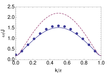
Figure 4: One particle dispersion of model (26) at $\delta=0.048$. The full dots are exact diagonalization data of Augier et al. (1997) obtained for a chain of $L=28$ sites (reproduction with permission of the authors). Our method is tested using only finite size energies up to $L=12$. The dashed curve is the result of our method assuming a triplet of fermions with effective ABC, while the continuous curve assumes a triplet of bosons with effective PBC.

IV.3 Spin-1 model with single ion anisotropy

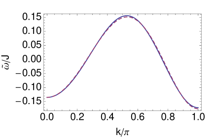
Figure 5: One particle dispersion for model Eq. (27) in the large-$D$ phase ($D=7.4$). Only the part of the function corresponding to Fourier cosine coefficients $c_{n}$ $n>1$ are shown. The continuous curve is the result of third order perturbation theory Eq. (28) without the $\cos\left(k\right)$ term. Perturbation theory is basically exact for such value of $D$ according to Golinelli et al. (1992). Our procedure is tested using finite size energies (obtained by Lanczos method) of short chains from $L=2,3,\ldots$up to $L=12$ and later discarding the $\cos\left(k\right)$ term from the dispersion. The dashed curve is our result assuming the dispersion is a doublet of bosonic particle and effective PBC. Assuming a doublet of Fermi particles and ABC one obtains similar accuracy although the $L^{2}\left(\left[0,\pi\right]\right)$ norm distance with dispersion (28) favors the bosons (distance $0.049$ against $0.078$).

As we have shown, our methods can be successfully applied to spin-1/2 chains only when the dispersion is even and of period $\pi$. This is the case for the pure Heisenberg model and for dimerized models as the one of Eq. (26). What about spin-1 chains? For PBC and even size the theorem by Lieb and Mattis Lieb and Mattis (1962) tells us that the ground state of a generic antiferromagnetic Heisenberg model belongs to the total spin zero sector and is unique. For odd sizes an antiferromagnet with PBC is frustrated and the theorem does not apply. However we have numerically verified that also for odd sizes the ground state belongs to the total spin zero sector (this is consistent with the VBS description and with the fact that every spin-1 can be thought of a symmetric combination of two spin-1/2, and so any chain contains an even number of spin-1/2). This suggests that we could use ground state energies both for even and odd sizes and re-construct completely the dispersion. However there is still a problem with this approach. The ground state energy for the single site problem is not clearly defined. If the model admits a quasi-free approximation, the $L=1$ ground state energy is given by $E_{1}=\pm\left(\nu/2\right)S_{1}\left(\omega_{k}\right)=\pm\left(\nu/2\right)\omega_{\vartheta}$ (plus or minus refers to Bosons or Fermion respectively). Using the inversion Eq. (14) we see that, $S_{1}\left(f\right)$ enters only in the definition of the first Fourier coefficient $a_{1}$. So a missing $S_{1}\left(f\right)$ allows to specify the function up to an additive $\cos\left(k\right)$ term. This term could be fixed by other means, such as obtaining the value of the dispersion at a given momentum. Let us analyze a concrete example.

Consider the spin-1 model with single ion anisotropy

$$H=J\sum_{i=1}^{L}\left[\mathbf{S}_{i}\cdot\mathbf{S}_{i+1}+D\left(S_{i}^{z}\right)^{2}\right]\,.$$ (27)

where $\mathbf{S}_{i}$ are now spin-1 operator. In order to test our method we consider the model for large $D$ where perturbation theory is applicable and an analytic expression for the dispersion is available. When $D=\infty$ the ground state is given by $|0,0,\ldots,0\rangle$, and excitations form a doublet of degenerate states with the spin at one site flipped to $+1$ or $-1$, i.e. $|0,0,\ldots,\pm 1,\ldots,0\rangle$. A finite large $D$, removes translation degeneracy and one obtains a doubly degenerate band $\omega\left(k\right)$. This picture remains valid in the whole, so-called, large-$D$ phase, which is separated by the Haldane phase roughly at $D_{c}\simeq 1$ (see Chen et al. (2003) for details on the phase diagram). In the large-$D$ phase one can use perturbation theory to obtain the doubly degenerate dispersion. A third order calculation has been performed Papanicolau and Spathis (1990) with the result

$$\frac{\omega\left(k\right)}{J}=D+2\cos\left(k\right)+\frac{1}{D}\left[1+2\sin\left(k\right)^{2}\right]+\\ \frac{1}{D^{2}}\left[2\sin\left(k\right)^{2}-\frac{1}{2}(1+8\sin\left(k\right)^{2})\cos\left(k\right)\right]+O\left(D^{-3}\right)$$ (28)

We re-write the dispersion as

$$\frac{\omega\left(k\right)}{J}=\left(D+\frac{2}{D}+\frac{1}{D^{2}}\right)+2\left(1-\frac{3}{4D^{2}}\right)\cos\left(k\right)\\ -\frac{1+D}{D^{2}}\cos\left(2k\right)+\frac{1}{D^{2}}\cos\left(3k\right)+O\left(D^{-3}\right)\,,$$ (29)

in order to make clear the Fourier (cosine) coefficients of the dispersion. Using a Lanczos algorithm we computed the ground state energy of the model (27) for $L=2,3,\ldots,12$. For what we have said, using the inversion Eq. (14) we can reconstruct the band up to a cosine term. In figure 5 we show the result for the reconstructed band compared to the dispersion Eq. (29) both without the $\cos\left(k\right)$ term and the agreement is excellent. As noticed previously, the $\cos\left(k\right)$ term can be fixed by other means.

V Conclusions

In this article we showed that a lot more information than currently believed, is encoded in the ground state energy density at finite size $e_{L}$. In particular we provided a method able to reconstruct an approximate one-particle dispersion for any one-dimensional quantum system, given some finite size numerical data $\left\{e_{L}\right\}$. The dispersion reconstructed with this procedure is optimal in the sense that it is the unique trigonometric polynomial of degree $L_{\mathrm{max}}$ ($L_{\mathrm{max}}$ being the number of energy data) consistent with the observed data $\left\{e_{L}\right\}$. Equivalently the method produces a quasi-free Hamiltonian which has the same ground state energy densities as the observed values $\left\{e_{L}\right\}$. This method is exact if the model has some sort of quasi-free representation, and it converges very rapidly increasing $L_{\mathrm{max}}$ so that very few data are sufficient (using 10 energy data gives already very good results). We also provided a simple criterion to assess whether such a quasi-free approximation is feasible in the first place. As a side effect, simply looking at the sequence $\left\{e_{L}\right\}$ this method is able to assess whether effective quasiparticles are either boson or fermions with effective periodic or anti-periodic boundary conditions.

Since the Casimir force is specified (up to a constant) by the energies $\left\{e_{L}\right\}$, from a physical point of view the procedure presented consists on reconstructing the one-particle dispersion given the Casimir force.

Further developments in this direction include the possibility of extending these ideas to higher dimension and testing the procedure on other strongly correlated systems.