Soumya Kundu Nikolai Sinitsyn Scott Backhaus
                             University of Michigan Los Alamos National Laboratory Los Alamos National Laboratory
                             Ann Arbor, USA Los Alamos, USA Los Alamos, USA
                             soumyak@umich.edu sinitsyn@lanl.gov backhaus@lanl.gov

                             Ian Hiskens
                             University of Michigan
                             Ann Arbor, USA
                             hiskens@umich.edu

Abstract - As the penetration of intermittent energy sources grows substantially, loads will be required to play an increasingly important role in compensating the fast time-scale fluctuations in generated power. Recent numerical modeling of thermostatically controlled loads (TCLs) has demonstrated that such load following is feasible, but analytical models that satisfactorily quantify the aggregate power consumption of a group of TCLs are desired to enable controller design. We develop such a model for the aggregate power response of a homogeneous population of TCLs to uniform variation of all TCL setpoints. A linearized model of the response is derived, and a linear quadratic regulator (LQR) has been designed. Using the TCL setpoint as the control input, the LQR enables aggregate power to track reference signals that exhibit step, ramp and sinusoidal variations. Although much of the work assumes a homogeneous population of TCLs with deterministic dynamics, we also propose a method for probing the dynamics of systems where load characteristics are not well known.

Keywords - Load modeling; load control; renewable energy; linear quadratic regulator.

1 INTRODUCTION

AS more renewable power generation is added to power systems, concerns for grid reliability increase due to the intermittency and non-dispatchability associated with such sources. Conventional power generators have difficulty in manoeuvering to compensate for the variability in the power output from renewable sources. On the other hand, electrical loads offer the possibility of providing the required generation-balancing ancillary services. It is feasible for electrical loads to compensate for energy imbalance much more quickly than conventional generators, which are often constrained by physical ramp rates.

A population of thermostatically controlled loads (TCLs) is well matched to the role of load following. Research into the behavior of TCLs began with the work of [1] and [2], who proposed models to capture the hybid dynamics of each thermostat in the population. The aggregate dynamic response of such loads was investigated by [4], who derived a coupled ordinary and partial differential equation (Fokker-Planck equation) model. The model was derived by first assuming a homogeneous group of thermostats (all thermostats having the same parameters), and then extended using perturbation analysis to obtain the model for a non-homogeneous group of thermostats. In [5], a discrete-time model of the dynamics of the temperatures of individual thermostats was derived, assuming no external random influence. That work was later extended by [6] to introduce random influences and heterogeneity.

Although the traditional focus has been on direct load control methods that directly interrupt power to all loads, recent work in [3] proposed hysteresis-based control by manipulating the thermostat setpoint of all loads in the population with a common signal. While it is difficult to keep track of the temperature and power demands of individual loads in the population, the probability of each load being in a given state (ON - drawing power or OFF - not drawing any power) can be estimated rather accurately. System identification techniques were used in [3] to obtain an aggregate linear TCL model, which was then employed in a minimum variance control law to demonstrate the load following capability of a population of TCLs.

In this paper, we derive a transfer function relating the aggregate response of a homogeneous group of TCLs to disturbances that are applied uniformly to the thermostat setpoints of all TCLs. We start from the hybrid temperature dynamics of individual thermostats in the population, and derive the steady-state probability density functions of loads being in the ON or OFF states. Using these probabilities we calculate aggregate power response to a setpoint change. We linearize the response and design a linear quadratic regulator to achieve reference tracking by the aggregate power demand. While our analytical model assumes a homogeneous population of loads, numerical studies are proposed to explore situations where there is noise and heterogeneity.

2 STEADY STATE DISTRIBUTION OF LOADS

2.1 Model development

The dynamic behavior of the temperature $\theta(t)$ of a thermostatically controlled cooling-load (TCL), in the ON and OFF state and in the absence of noise, can be modeled by [5],

$$\dot{\theta}=\left\{\begin{array}[]{ll}-\frac{1}{CR}\left(\theta-\theta_{amb}+PR\right),&\text{ON state}\\ &\\ -\frac{1}{CR}\left(\theta-\theta_{amb}\right),&\text{OFF state}\end{array}\right.$$ (1)

where $\theta_{amb}$ is the ambient temperature, $C$ is the thermal capacitance, $R$ is the thermal resistance, and $P$ is the power drawn by the TCL when in the ON state. This response is shown in Figure 2.1.

Figure 1: Dynamics of temperature of a thermostatic load.

In steady state the cooling period drives a load from temperature $\theta_{+}$ to temperature $\theta_{-}$. Thus solving (1) with initial condition $\theta(0)=\theta_{+}$ gives

$$\theta(t)=\left(\theta_{amb}-PR\right)\left(1-e^{-\frac{t}{CR}}\right)+\theta_{+}e^{-\frac{t}{CR}}.$$ (2)

From (2) we can calculate the steady state cooling time $T_{c}$ by equating $\theta(T_{c})$ to $\theta_{-}$,

$$T_{c}={CR}\ln\left(\frac{PR+\theta_{+}-\theta_{amb}}{PR+\theta_{-}-\theta_{amb}}\right).$$ (3)

A similar calculation for the heating time gives,

$$T_{h}={CR}\ln\left(\frac{\theta_{amb}-\theta_{-}}{\theta_{amb}-\theta_{+}}\right).$$ (4)

In general, the expressions for the times $t_{c}(\theta_{f})$ and $t_{h}(\theta_{f})$ taken to reach some intermediate temperature $\theta_{f}$ during the cooling and heating periods, respectively, are,

$$t_{c}(\theta_{f}) ={CR}\ln\left(\frac{PR+\theta_{+}-\theta_{amb}}{PR+\theta_{f}-\theta_{amb}}\right)$$ (5)

$$t_{h}(\theta_{f}) ={CR}\ln\left(\frac{\theta_{amb}-\theta_{-}}{\theta_{amb}-\theta_{f}}\right).$$ (6)

For a homogeneous set of TCL in steady state, the number of loads in the ON and OFF states, $N_{c}$ and $N_{h}$ respectively, will be proportional to their respective cooling and heating time periods $T_{c}$ and $T_{h}$. In the absence of any appreciable noise, which ensures that all the loads are within the temperature deadband, $N_{h}+N_{c}=N$, we obtain,

$$N_{c} =\frac{T_{c}}{T_{c}+T_{h}}N$$ (7)

$$N_{h} =\frac{T_{h}}{T_{c}+T_{h}}N$$ (8)

By analogy, it follows that the number of ON-loads $n_{c}(\theta)$ within a temperature band of $[\theta,\;\theta_{+}]$ is proportional to the time taken $t_{c}(\theta)$ to cool a load down from $\theta_{+}$ to an arbitrary temperature $\theta\geq\theta_{-}$,

$$n_{c}(\theta) =t_{c}(\theta)\frac{N_{c}}{T_{c}}$$

$$=t_{c}(\theta)\frac{N}{T_{c}+T_{h}}$$ (9)

where (8) was used to obtain (9). Likewise,

$$n_{h}(\theta)=t_{h}(\theta)\frac{N}{T_{c}+T_{h}}.$$ (10)

We will denote the ON probability density function by $f_{1}(\theta)$ and the OFF probability density function by $f_{0}(\theta)$, while the corresponding cumulative distribution functions are denoted $F_{1}(\theta)$ and $F_{0}(\theta)$, respectively. It is to be noted that, $F_{0}(\theta)$ is the probability of a load being in OFF state and having a temperature $\theta\in[\theta_{-},\theta]$ while $F_{1}(\theta)$ is the probability of a load being in ON state and having a temperature $\theta\in[\theta_{-},\theta]$. Thus, $F_{0}(\theta)=n_{h}(\theta)/N$ and $F_{1}(\theta)=(N_{c}-n_{c}(\theta))/N$. We can therefore write,

$$f_{0}(\theta) =\frac{dF_{0}(\theta)}{d\theta}=\frac{d}{d\theta}\left(\frac{n_{h}(\theta)}{N}\right)$$

$$=\frac{1}{N}\frac{dt_{h}(\theta)}{d\theta}\frac{N}{T_{c}+T_{h}}$$

$$=\frac{1}{T_{c}+T_{h}}\frac{dt_{h}(\theta)}{d\theta}$$

$$=\frac{CR}{(T_{c}+T_{h})(\theta_{amb}-\theta)}$$ (11)

and

$$f_{1}(\theta) =\frac{dF_{1}(\theta)}{d\theta}=\frac{d}{d\theta}\left(\frac{N_{c}-n_{c}(\theta)}{N}\right)$$

$$=\frac{CR}{(T_{c}+T_{h})(PR+\theta-\theta_{amb})}.$$ (12)

2.2 Simulation

Figure 2.2 shows a comparison of the densities calculated using (11) and (12) and those computed from actual simulation of the dynamics of a population of 10,000 TCLs that included a small amount of noise. The result suggests that the assumptions underlying (11) and (12) are realistic.

Figure 2: Steady state densities.

3 SETPOINT VARIATION

Control of active power can be achieved by making a uniform adjustment to the temperature setpoint of all loads within a large population [3]. It is assumed that the temperature deadband moves in unison with the setpoint. Figure 3 shows the change in the aggregate power consumption of a population of TCLs for a small step change in the setpoint of all devices. The resulting transient variations in the OFF-state and ON-state distributions for the population are shown in Figure 3.

Figure 3: Change in aggregate power consumption due to a step change in temperature setpoint.

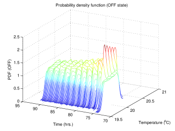
(a) OFF-state distribution.

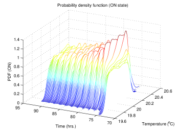
(b) ON-state distribution.

Figure 4: Variation in distribution of loads due to setpoint disturbance.

The aggregate power consumption at any instant in time is proportional to the number of loads in the ON state at that instant. The first step in quantifying the change in power due to a step change in setpoint is therefore to analyze the behavior of the TCL probability distributions. Figure 3 depicts a situation where the setpoint has just been increased. The original deadband ranged from $\theta_{-}^{0}$ to $\theta_{+}^{0}$, with the setpoint at $(\theta_{-}^{0}+\theta_{+}^{0})/2$. After the positive step change, the new deadband lies between $\theta_{-}$ to $\theta_{+}$, with the deadband width $\Delta=\theta_{+}^{0}-\theta_{-}^{0}=\theta_{+}-\theta_{-}$ remaining unchanged. The setpoint is shifted by $\delta=\theta_{-}-\theta_{-}^{0}=\theta_{+}-\theta_{+}^{0}$. To solve for the power consumption, we need to consider four different TCL starting conditions immediately after the step change in setpoint, i.e. $a$-$d$ in Figure 3. Using Laplace transforms, we compute the time dependence of the power consumption for each of these loads (shown in Figure 3) and then compute the total power consumption by integrating over the distributions $f_{0}$ and $f_{1}$. At the instant the step change in applied, the temperatures of loads at points $a$, $b$, $c$ and $d$ are $\theta_{a},\theta_{b},\theta_{c}$ and $\theta_{d}$, respectively.

Figure 5: Different points of interest on the density curves.

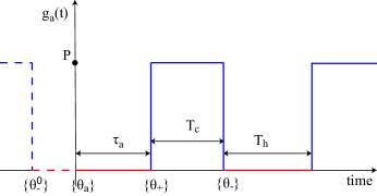
(a) Power waveform at point $a$.

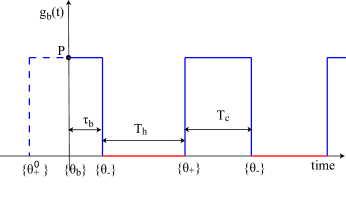
(b) Power waveform at point $b$.

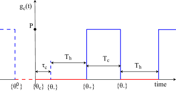
(c) Power waveform at point $c$.

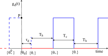
(d) Power waveform at point $d$.

Figure 6: Power waveforms at four different points marked in Figure 3.

The power consumption $g_{a}(t,\tau_{a})$ of the load at $a$ starting from the instant when the step change in setpoint is applied is shown in Figure 6(a). All the loads in the OFF-state and having a temperature between $\theta_{-}$ and $\theta_{+}^{0}$ at the instant when the deadband shift occurs will have power waveforms similar in nature to $g_{a}(t,\tau_{a})$. Thus the load at $a$ typifies the behavior of all the loads lying on the OFF-state density curve between $\theta_{-}$ and $\theta_{+}^{0}$. The same argument applies for loads at points $b$, $c$ and $d$. Figures 6(a)-6(d) illustrate the general nature of the power waveforms of the loads in all four regions, marked by $a$, $b$, $c$ and $d$ in Figure 3.

The Laplace transform of $g_{a}(t,\tau_{a})$ is

$$\mathbf{G}_{a}(s,\tau_{a})=e^{-s\tau_{a}}\mathbf{G}(s)$$

where

$$\mathbf{G}(s)=\frac{P(1-e^{-sT_{c}})}{s(1-e^{-s(T_{c}+T_{h})})}$$

and $\tau_{a}=T_{h}-t_{h}(\theta_{a})$, with $t_{h}(\theta_{a})$ given by (6). Averaging over all such loads (represented by $a$) on the OFF density curve between temperatures $\theta_{-}$ and $\theta_{+}^{0}$, we obtain the Laplace transform of the average power demand,

$$\mathbf{P}_{a}(s)=\int_{\theta_{-}}^{\theta_{+}^{0}}{f_{0}(\theta_{a})\mathbf{G}_{a}(s,\tau_{a})}d\theta_{a}$$ (13)

where $f_{0}(\theta_{a})$ can be computed from (11).

In Figure 6(b), a load at point $b$ on the ON density curve in Figure 3 has power consumption $g_{b}(t,\tau_{b})$, where $\tau_{b}=T_{c}-t_{c}(\theta_{b})$, and $t_{c}(\theta_{b})$ is given by (5). The Laplace transform is,

$$\mathbf{G}_{b}(s,\tau_{b})=\Big{(}e^{s(T_{c}-\tau_{b})}\mathbf{G}(s)-\frac{P}{s}\big{(}e^{s\left(T_{c}-\tau_{b}\right)}-1\big{)}\Big{)}.$$

We can compute the average power demand of all the loads represented by $b$ as

$$\mathbf{P}_{b}(s)=\int_{\theta_{-}}^{\theta_{+}^{0}}f_{1}(\theta_{b})\mathbf{G}_{b}(s,\tau_{b})d\theta_{b}.$$ (14)

In Figure 6(c), the power consumption $g_{c}(t,\tau_{c})$ of a load at point $c$ on the OFF density curve in Figure 3 has the Laplace transform

$$\mathbf{G}_{c}(s,\tau_{c})=e^{-s(T_{h}+\tau_{c})}\mathbf{G}(s),$$

where $\tau_{c}=CR\ln\left(\frac{\theta_{amb}-\theta_{-}}{\theta_{amb}-\theta_{c}}\right)$. The average power demand of the loads represented by the point $c$ is then given by

$$\mathbf{P}_{c}(s)=\int_{\theta_{-}^{0}}^{\theta_{-}}f_{0}(\theta_{c})\mathbf{G}_{c}(s,\tau_{c})d\theta_{c}$$ (15)

Figure 6(d) depicts the situation of a load at point $d$ on the ON density curve, that suddenly switches to the OFF state as the deadband is shifted (for now we assume the deadband is shifted to the right, i.e., there is an increase in the setpoint). The power consumption $g_{d}(t)$ has the Laplace transform

$$\mathbf{G}_{d}(s,\tau_{d})=e^{-s(T_{h}+\tau_{d})}\mathbf{G}(s),$$

where the dynamics in (1) can be solved for $\tau_{d}=CR\ln\left(\frac{\theta_{amb}-\theta_{d}}{\theta_{amb}-\theta_{-}}\right)$. The average power demand of the loads characterized by point $d$ in Figure 3 is then given by

$$\mathbf{P}_{d}(s)=\int_{\theta_{-}^{0}}^{\theta_{-}}f_{1}(\theta_{d})\mathbf{G}_{d}(s,\tau_{d})d\theta_{d}.$$ (16)

The average power demand of the whole population becomes,

$$\mathbf{P}_{avg}(s)=\mathbf{P}_{a}(s)+\mathbf{P}_{b}(s)+\mathbf{P}_{c}(s)+\mathbf{P}_{d}(s).$$ (17)

Using (13), (14), (15) and (16) we obtain an expression for $\mathbf{P}_{avg}(s)$ that is rather complex. It is hard, and perhaps even impossible, to obtain the inverse Laplace transform. However, with the assistance of MATHEMATICA^®, $\mathbf{P}_{avg}(s)$ may be expanded as a series in $s$. We also make use of the assumptions,

$$\Delta\ll(\theta_{s}-\theta_{amb}+PR)$$

$$\Delta\ll(\theta_{amb}-\theta_{s})$$

$$\delta\ll\Delta$$

where $\theta_{s}$ is the setpoint temperature. Note that the first two assumptions require that the deadband width is small, while the third assumption requires that the shift in the deadband is small relative to the deadband width. This latter assumption ensures that the load densities are not perturbed far from their steady-state forms. Accordingly, the steady-state power consumption is given by

$$P_{avg,ss}\approx\frac{(\theta_{amb}-\theta_{+})N}{\eta R},$$

where $\eta$ is the electrical efficiency of the cooling equipment and $N$ is the population size. The deviation in power response can be approximated by

$$\mathbf{P}_{tot}(s)\approx-\left(\frac{d}{s}+\frac{\omega A_{\Delta}}{s^{2}+\omega^{2}}\right)\delta$$ (18)

where

$$A_{\Delta}=\frac{5\sqrt{15}C(\theta_{amb}-\theta_{+})(PR-\theta_{amb}+\theta_{+})}{\eta\big{(}P^{2}R^{2}+3PR(\theta_{amb}-\theta_{+})-3(\theta_{amb}-\theta_{+})^{2}\big{)}^{3/2}}$$

$$\qquad\qquad\qquad\times\frac{(3PR-\theta_{amb}+\theta_{+})N}{(T_{c0}+T_{h0})},$$

$$\omega=\frac{2\sqrt{15}(\theta_{amb}-\theta_{+})(PR-\theta_{amb}+\theta_{+})}{CR\Delta\sqrt{P^{2}R^{2}+3PR(\theta_{amb}-\theta_{+})-3(\theta_{amb}-\theta_{+})^{2}}},$$

$$d=\frac{N}{\eta R}.$$

and $T_{c0}$ and $T_{h0}$ are the original (prior to the setpoint shift) steady-state cooling and heating times, respectively, given by (3) and (4). The transfer function for this linear model is,

$$\mathbf{T}(s)=\frac{\mathbf{P}_{tot}(s)}{\delta/s}=-\Big{(}d+\frac{A_{\Delta}\omega s}{s^{2}+\omega^{2}}\Big{)}.$$

Due to the assumptions of low-noise and homogeneity, our analytical model is undamped. The actual system, on the other hand, experiences both heterogeneity and noise, and therefore will exhibit a damped response. In order to capture that effect, we have chosen to add a damping term $\sigma$ (to be estimated on-line) into the model, giving

$$\mathbf{T}(s)=-\Big{(}d+\frac{s\omega A_{\Delta}}{(s+\sigma)^{2}+\omega^{2}}\Big{)}.$$ (19)

Figure 3 shows a comparison between the response calculated from the model (19) and the true response to a step change in the setpoint obtained from simulation. A damping coefficient of 0.002 min^-1 was added, as that value gave a close match to the decay in the actual system response.

Figure 7: Comparison of the approximate model with the actual simulation, for the same setpoint disturbance as in Figure 3.

4 CONTROL LAW

The TCL load controller, described by the transfer function (19), can also be expressed in state-space form,

$$\dot{x} =\mathbf{A}x+\mathbf{B}u$$

$$y =\mathbf{C}x+\mathbf{D}u$$

where the input $u(t)$ is the shift in the deadband of all TCLs, and the output $y(t)$ is the change in the total power demand from the steady-state value. The state-space matrices are given by

$$\mathbf{A} =\begin{bmatrix}-2\sigma&-\omega\\ \frac{\sigma^{2}+\omega^{2}}{\omega}&0\end{bmatrix}, \mathbf{B} =\begin{bmatrix}\omega A_{\Delta}\\ 0\end{bmatrix},$$

$$\mathbf{C} =\begin{bmatrix}-1&0\end{bmatrix}, \mathbf{D} =-d.$$

Our goal is to design a controller using the linear quadratic regulator (LQR) approach [7] to track an exogenous reference $y_{d}$. We observe that the system has an open-loop zero very close to the imaginary axis ($d\ll\omega A_{\Delta}$) and hence we need to use an integral controller. Considering the integral of the output error $e=(y-y_{d})$, where $y_{d}$ is the reference, as the third state $w(t)=\int_{0}^{t}(y(\tau)-y_{d}(\tau))d\tau$ of the system, the modified state-space model becomes

$$\dot{\underline{x}} ={\bf\underline{A}}\,\underline{x}+{\bf\underline{B}}u+{\bf E}\,y_{d}$$

$$y ={\bf\underline{C}}\,\underline{x}+{\bf\underline{D}}u$$

where $\underline{x}=[x\quad w]^{\top}$ and,

$${\bf\underline{A}} =\begin{bmatrix}{\bf A}&{\bf 0}_{2\times 1}\\ {\bf C}&0\end{bmatrix}, {\bf\underline{B}} =\begin{bmatrix}{\bf B}\\ {\bf D}\end{bmatrix},$$

$${\bf\underline{C}} =\begin{bmatrix}{\bf C}&0\end{bmatrix}, {\bf\underline{D}} ={\bf D},\quad{\bf E}=\begin{bmatrix}{\bf 0}_{2\times 1}\\ -1\end{bmatrix}.$$

Minimizing the cost function

$$J=\int^{\infty}_{0}\big{(}\underline{x}(t)^{\top}Q\underline{x}(t)+u(t)^{2}R\big{)}dt$$

where $Q\geq{\bf 0}_{3\times 3}$ and $R>0$ are design variables, we obtain the optimal control law $u(t)$ of the form

$$u=-(\mathbf{K}\,\underline{x}+\mathbf{G}\,y_{d}),$$

with $\mathbf{G}$ a pre-compensator gain chosen to ensure unity DC gain. Since we can only measure the output $y(t)$ and the third state $w(t)$, the other two states are estimated using a linear quadratic estimator [7] which has the state-space form,

$$\dot{\hat{x}} =\mathbf{A}\,\hat{x}+\mathbf{B}u+\mathbf{L}(y-y_{d})$$

$$\hat{y} =\mathbf{C}\,\hat{x}+\mathbf{D}u$$

$$u =-\mathbf{K}\,\begin{bmatrix}\hat{x}\\ w\end{bmatrix}+\mathbf{G}\,y_{d}.$$

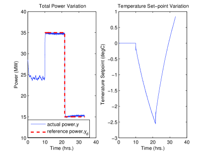
(a) Response to step reference and the control input

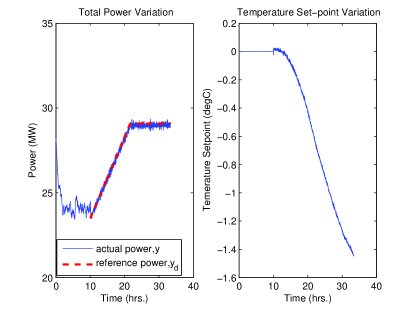
(b) Response to ramp reference and the control input

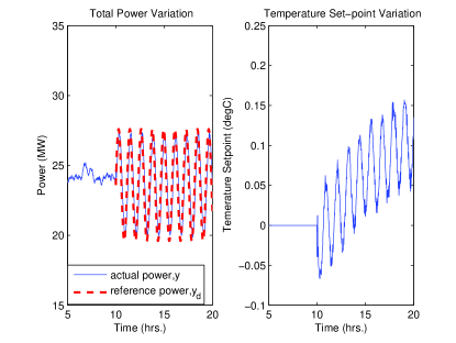
(c) Response to sinusoidal reference and the control input

Figure 8: Reference tracking achieved through setpoint shift

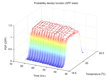
(a) OFF-state distribution.

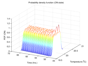
(b) ON-state distribution.

Figure 9: Variation in distribution of loads under the influence of the controller.

The plots in Figure 4 show that the controller can be used to force the aggregate power demand of the TCL population to track a range of reference signals. The transient variations in the ON-state and OFF-state populations are shown in Figure 4. In comparison with the uncontrolled response of Figure 3, it can be seen that the controller suppresses the lengthy oscillations. Figure 4 shows that in presence of the controller, the distribution of loads almost always remains close to steady state, justifying an assumption made during the derivation of the model.

5 HETEROGENEITY AND NOISE

The work presented in previous sections assumes a homogeneous population of loads with deterministic dynamics. The analysis remains valid if we consider the possibility of grouping a large number loads having closely matched parameters, and if there is very low noise in the system. When such assumptions no longer remain valid, we cannot design a tracking controller based on the developed model. In such cases, however, we propose a probing method that can balance over- or under-production of energy over a certain duration of time.

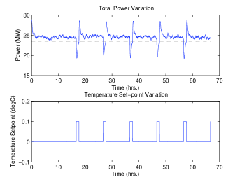
(a) Power response to short duration pulses.

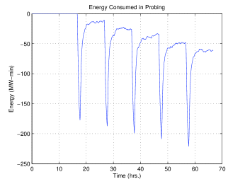
(b) Energy consumed (over nominal) in response to such pulses. (A negative value means energy is delivered.)

Figure 10: Energy consumption in the probing method.

Figure 10(a) can be used to explain the probing method. The temperature setpoint is increased and held at that value for a short duration and then returned to its original value. The system is probed by short pulses spaced reasonably far from each other in time. The energy delivered during such probing is monitored, with Figure 10(b) providing an illustration. It can be seen that the energy consumed, relative to the nominal consumption, is actually negative suggesting that energy is “delivered” by the loads when probed with positive pulses. Knowing that over a certain duration a certain amount of energy can be delivered by the loads, the pulses can be scheduled to balance any under-generation. Similarly, over-generation can be balanced using negative pulses.

6 CONCLUSION

In this paper we have analytically derived a transfer function relating the change in aggregate power demand of a population of TCLs to a change in thermostat setpoint applied to all TCLs in unison. We have designed a linear quadratic regulator to enable the aggregate power demand to track reference signals. This suggests the derived aggregate response model could be used to allow load to track fluctuations in renewable generation. The analysis has been based on the assumptions that the TCL population is homogeneous and that the noise level is insignificant. When such assumptions do not hold, we propose a probing method that can be used to perform energy balance. Further studies are required to incorporate the effects of heterogeneity and noise into the model. Those extensions are important for determining the damping coefficient.

Similar analysis can be used to establish the aggregate characteristics of groups of plug-in electric vehicles, another candidate for compensating the variability in renewable generation.

REFERENCES

- [1] Ihara S and Schweppe FC, “Physically based modelling of cold load pickup”, IEEE Trans Power App Syst, 100:4142 50, 1981.
- [2] Chong CY and Debs AS, “Statistical synthesis of power system functional load models”, 18th IEEE conference on decision and control, 1979.
- [3] D. S. Callaway, “Tapping the energy storage potential in electric loads to deliver load following and regulation, with application to wind energy”, Energy Conversion & Management, 50(9): 1389-1400, May 2009.
- [4] Malhamé R and Chong CY, “Electric-load model synthesis by diffusion approximation of a high-order hybrid-state stochastic system”, IEEE Trans Automat Contr, 30: 854-60, 1985.
- [5] Mortensen RE and Haggerty KP, “A stochastic computer model for heating and cooling loads”, IEEE Trans Power Syst, 3: 1213-9, 1988.
- [6] Uçak C and Çağlar R, “The effects of load parameter dispersion and direct load control actions on aggregated load”, POWERCON 98, 1998.
- [7] B. D. O. Anderson and J. B. Moore, “Optimal Control: Linear Quadratic Methods”, Prentice-Hall, 1990.