Mildly mixed coupled models vs. WMAP7 data

Abstract

Mildly mixed coupled models include massive $\nu$’s and CDM–DE coupling. We present new tests of their likelihood vs. recent data including WMAP7, confirming it to exceed $\Lambda$CDM, although at $\sim 2$–$\sigma$’s. We then show the impact on the physics of the dark components of $\nu$–mass detection in ³H $\beta$–decay or $0\nu\beta\beta$–decay experiments.

1 Spectral distorsions

Cosmological data (apart ⁷LI abundance) are nicely fitted by $\Lambda$CDM, a model which however has severe fine tuning and coincidence problems. Here we therefore discuss an alternative easing these problems: that, symoultaneously, neutrinos ($\nu$) have mass, and DE is a scalar field $\phi$ self–interacting and interacting with Cold Dark Matter (CDM). To our knowledge, this is the only alternative whose likelihood, although marginally, exceeds $\Lambda$CDM.

An energy transfer from CDM to Dark Energy (DE) causes significant distorsions of $C_{l}$ and $P(k)$ spectra in respect to $\Lambda$CDM, but allows DE to be a significant cosmic component since ever; distortions are also caused by $\nu$ masses, in the range $M_{\nu}=\sum_{i}m_{i}\sim 1$ eV. These two distorsions tend however to compensate and compensation allows to fit data better than $\Lambda$CDM (Figure 1 shows this for CMB anisotropy spectrum).

This yields models including a slight amount of Hot Dark Matter (typically $\Omega_{h}\sim 0.01$); they are then Mildly Mixed and Coupled (MMC) models.

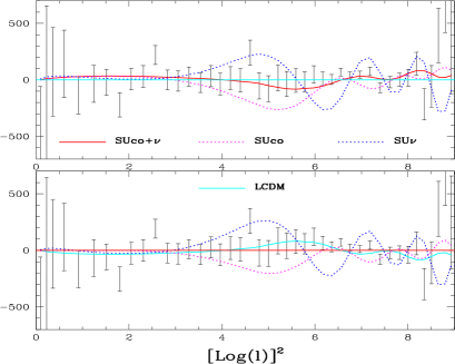
Figure 1: $\Lambda$CDM and MMC $C_{l}$ compared. In the upper (lower) plot $C_{l}$ are normalized to $\Lambda$CDM (the best fitting SUGRA model including coupling and massive $\nu$’s). $C_{l}$ obtained with either coupling or massive $\nu$’s only are also shown. The error bars are a sampling of WMAP7 $C_{l}$ data.

2 Potentials & coupling

Among possible CDM–DE couplings [1], we consider the option arising from Brans–Dickie gravity conformally transformed from the Jordan to the Einstein frame [2], just allowing for a generalized self–interaction potential. Then, while $T^{(c)~{}\mu}_{~{}~{}~{}~{}\nu;\mu}+T^{(de)~{}\mu}_{~{}~{}~{}\,~{}~{}\nu;\mu}=0\,$, it is

$$T^{(de)~{}\mu}_{~{}~{}~{}\,~{}~{}\nu;\mu}=+CT^{(c)}\phi_{,\nu}~{},~{}~{}T^{(c)~{}\mu}_{~{}~{}~{}~{}\nu;\mu}=-CT^{(c)}\phi_{,\nu}~{},$$ (1)

($T^{(c,de)}_{\mu\nu}:$ CDM and DE stress–energy tensors, $T^{(c,de)}:$ their traces) with a coupling

$$C=(16\pi/3)^{1/2}\beta/m_{p}$$ (2)

($m_{P}:$ Planck mass). Ratra–Peebles (RP, [3]) or SUGRA [4] potentials

$$V(\phi)=(\Lambda/\phi)^{\alpha}~{}~{}~{}~{}~{}~{}~{}~{}~{}~{}~{}~{}~{}~{}~{}~{}~{}~{}~{}~{}~{}~{}~{}~{}(RP)$$ (3)

$$V(\phi)=(\Lambda/\phi)^{\alpha}\exp(4\pi\phi^{2}/m_{p})~{}~{}~{}(SUGRA)$$ (4)

are considered here, for $\phi$ self–interaction, so easing fine tuning. RP (SUGRA) yields a smooth (fast) dependence of the DE state parameter on redshift. For both potentials $\Lambda$ will be taken as a free parameter. Once the density parameter of DE is found, the valuse of $\alpha$ is also uniquely defined. Both these potentials also yield a dynamical rise from $\cal O$$(10^{-2})$ to unity of the DE/CDM ratio, at the eve of the present epoch, so easing coincidence as well. The natural scale for $C$ is then $\cal O$$(m_{p}^{-1})$; only in the presence of $\nu$ masses such range gets consistent with data.

3 Neutrino mass

Absolute $\nu$ masses can be measured through double beta decays ($0\nu\beta\beta$) or ³H $\beta$ decay [5, 6].

The former process is allowed only if $\nu$’s are Majorana spinors with mass, yielding

$$m_{\beta\beta}^{2}=\sum_{i}U_{ei}^{2}m_{i}={m_{e}^{2}}/{C_{mm}t^{\,0\nu\beta\beta}_{1/2}}$$ (5)

($U_{ei}:$ PMNS $\nu$ mixing matrix; $m_{e}:$ electron mass; $t^{0\nu\beta\beta}_{1/2}:$ decay half life). Here, the nuclear matrix element $C_{mm}$ causes the main uncertainties.

Using ⁷⁶Ge, the Heidelberg-Moscow (HM) [7] and the IGEX [8] experiments gave $t^{0\nu}_{1/2}>1.9\times 10^{25}y$ and $t^{0\nu}_{1/2}>1.6\times 10^{25}y$, respectively. However, a part of the HM theam claims a $t^{0\nu}$ detection yielding $m_{\beta\beta}\neq 0$ at $>5\sigma$’s. At $3\,\sigma$’s, this KK–claim reads $m_{\beta\beta}=(0.2-0.6)$eV [9].

The best limits on $m_{\beta}$ from ³H $\beta$–decay come from the Mainz and Troitsk experiments: $m_{\beta}<2.0\,$eV, at 95% C.L.). The experiment KATRIN [6] will soon improve the limit by one order of magnitude, being able to confirm the KK claim.

This is the range of masses needed to balance DE–CDM coupling, so yielding MMC models.

4 Methods & data

Here we show results of fits of MMC models to available cosmological data, performed by using the publicly available code CosmoMC [10]. The dataset combinations considered are: (i) WMAP7+BAO+$H_{o}$. (ii) WMAP7+BAO+SNIa. (iii) The same data plus the power spectrum of galaxy surveys.

The following parameters define the model:

{ $\omega_{b},\omega_{c},\theta,\tau,n_{s},\ln 10^{10}A_{s},\Lambda,\beta,M_{\nu}$ }

Here $\omega_{b,c}=\Omega_{b,c}h^{2}$, $\theta$ is the ratio of the comoving sound horizon at recombination to its distance, $\Lambda$ is the energy scale in RP or SUGRA potentials, $\beta$ yields the CDM–DE coupling, $\tau$ and $A$ have their usual meanings, while $\nu$–mass differences are neglected.

Results including in datasets SSDS “data” [11] will be also shown. Although used also in WMAP7 release [12], such “data” are obtained from observations by exploiting the Halofit expressions [13] for non–linear spectra. Such expressions are reliable within the frame of $\Lambda$CDM cosmologies, but could produce misleading results if the true cosmology is non–$\Lambda$CDM, as we envisage here. It does not come then as a surprise that these last results appear much less promising for MMC cosmologies.

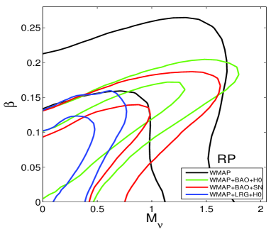
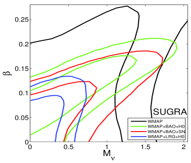
Figure 2: 1– & 2–$\sigma$ likelihood contours for various datasets. The red and green ones, using CMB and BAO data, plus either $H_{0}$ or SNIa constraints, confirm the correlation between $\beta$ and $M_{\nu}$. WMAP7 data only provide quite loose contours. Blue contours include SSDS spectral data (LRG). They are reported for the sake of completeness, but they assume Halofit spectral expressions, unsuitable to fit non–$\Lambda$CDM models.

——————————————————

Figure 3: Likelihood distribution on $\beta$, $\Lambda$, $M_{\nu}$ for various datasets (about then see the caption of the previous Figure). The upper (lower) panel is for RP (SUGRA) potential. Notice the near–detection of $\beta$ and that $\Lambda$ constraint are looser than in the absence of coupling.

5 Results

In Figure 2 we show 1– and 2–$\sigma$ marginalized likelihood curves in respect to various datasets (see caption) for RP and SUGRA potentials. The two panels exhibit just marginal quantitative shifts and, in the sequel, only RP results will be reported.

The strong degeneracy between $M_{\nu}$ and $\beta$ is confirmed, evident when CMB data are put together with low–$z$ data. If spectral SDSS data are used, the degeneracy is damped. As previously outlined, this is not a surprise and calls for an unbiased analysis of the huge SDSS sample.

In Figure 3 we show marginalized and average likelihood distributions on $\beta$ (coupling), $\Lambda$ (energy scale in potential) and $M_{\nu},$ when varying the dataset.

Both $\beta$ and $M_{\nu}$ plots exhibit a maximum at non–zero values. The maximum on $\beta$ persists even when spectral data are considered.

We then studied what effects would arise on cosmological parameters if the KK-claim is correct (Figure 4, upper panel) or the KATRIN experiment (Figure 4, lower panel) leads to $\nu$ mass detection. The two Figure differ for the range of $\nu$ mass considered.

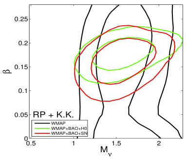
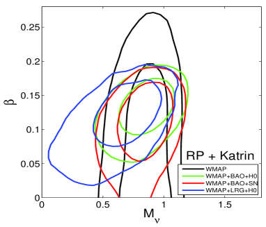
Figure 4: Likelihood distribution under the assumption of the validity of the KK–claim ($M_{\nu}=1.5$ eV; upper panel) or assuming the detection of $M_{\nu}=0.9$ by KATRIN (lower panel). The plots are reported for the RP potential only; in the SUGRA case there are no qualitative differences.

In the latter case we assumed $M_{\nu}\simeq 0.9~{}$eV and this leads to the area of top expectation, from cosmological data. On the contrary, the average KK–claim takes us above such area, although one should not forget that such claim could be quite consistent with our “KATRIN” assumption.

Let us however ooutline that, besides of being consistent with MMC models, such $\nu$–mass detections apparently imply the discovery of CDM-DE coupling, possibly at more than 3–$\sigma$’s and a final overcoming of the $\Lambda$CDM cosmology.

References

- [1] L. L. Honorez, B. A. Reid, O. Mena, L. Verde and R. Jimenez, JCAP 1009 (2010) 029.
- [2] L. Amendola, Phys. Rev. D 62, 043511 (2000); see also: T. Damour, G. W. Gibbons and C. Gundlach, Phys. Rev. Lett. 64, 123 (1990); T. Damour and C. Gundlach Phys. Rev. D 43, 3873 (1991)
- [3] B. Ratra and P. J. E. Peebles, Phys. Rev. D 37, 3406 (1988)
- [4] P. Brax and J. Martin, Phys. Lett. B 468, 40 (1999); P. Brax and J. Martin, Phys. Rev. D 61, 103502 (2000)
- [5] F. T. . Avignone, S. R. Elliott and J. Engel, Rev. Mod. Phys. 80 (2008) 481; G. L. Fogli et al., Phys. Rev. D 78 (2008) 033010
- [6] J. Bonn [KATRIN Collaboration], Prog. Part. Nucl. Phys. 64 (2010) 285.
- [7] L. Baudis et al., Phys. Rev. Lett. 83, 41 (1999); H. V. Klapdor-Kleingrothaus et al., Eur. Phys. J. A 12, 147 (2001)
- [8] C. E. Aalseth et al. [IGEX Collaboration], Phys. Rev. C 59, 2108 (1999); C. E. Aalseth et al. [IGEX Collaboration], Phys. Rev. D 65, 092007 (2002); C. E. Aalseth et al., Phys. Rev. D 70, 078302 (2004)
- [9] H. V. Klapdor-Kleingrothaus, I. V. Krivosheina, A. Dietz and O. Chkvorets, Phys. Lett. B 586, 198 (2004); H. V. Klapdor-Kleingrothaus, arXiv:hep-ph/0512263.
- [10] A. Lewis and S. Bridle, Phys. Rev. D 66, 103511 (2002)
- [11] B. A. Reid et al., Mon. Not. Roy. Astron. Soc. 404, 60 (2010)
- [12] E. Komatsu et al., arXiv:1001.4538
- [13] R. E. Smith et al. [The Virgo Consortium Collaboration], Mon. Not. Roy. Astron. Soc. 341 (2003) 1311