Supersymmetric mass spectra and the seesaw scale

Abstract

Supersymmetric mass spectra within two variants of the seesaw mechanism, commonly known as type-II and type-III seesaw, are calculated using full 2-loop RGEs and minimal Supergravity boundary conditions. The type-II seesaw is realized using one pair of $15$ and $\overline{15}$ superfields, while the type-III is realized using three copies of $24_{M}$ superfields. Using published, estimated errors on SUSY mass observables attainable at the LHC and in a combined LHC+ILC analysis, we calculate expected errors for the parameters of the models, most notably the seesaw scale. If SUSY particles are within the reach of the ILC, pure mSugra can be distinguished from mSugra plus type-II or type-III seesaw for nearly all relevant values of the seesaw scale. Even in the case when only the much less accurate LHC measurements are used, we find that indications for the seesaw can be found in favourable parts of the parameter space. Since our conclusions crucially depend on the reliability of the theoretically forecasted error bars, we discuss in some detail the accuracies which need to be achieved for the most important LHC and ILC observables before an analysis, such as the one presented here, can find any hints for type-II or type-III seesaw in SUSY spectra.

I Introduction

In the minimal supersymmetric extension of the standard model (MSSM) all soft SUSY breaking mass terms are treated as free parameters, to be fixed at the electro-weak scale. However, these soft parameters potentially contain a wealth of information about physics at the high scale and understanding the nature of SUSY breaking will become the main challenge, if signals of SUSY are found at the LHC. Highly precise mass measurements will be needed to distinguish between different SUSY breaking schemes such as “minimal supergravity” (mSugra) Chamseddine:1982jx ; Nilles:1983ge , anomaly mediated SUSY breaking (AMSB) Giudice:1998xp ; Chacko:1999am or gauge mediated SUSY breaking (GMSB) Giudice:1998bp , to name just the most familiar ones.

However, all of the models mentioned above break SUSY at energies inaccessible for collider experiments. Thus, theoretical extrapolations from the TeV scale to the high energy scale will be needed and any “test” of SUSY breaking schemes can at best take the form of a consistency check. Based on the results of AguilarSaavedra:2001rg ; Weiglein:2004hn ; AguilarSaavedra:2005pw detailed calculations have been done, quantifying the accuracy with which such tests can be done using data from LHC and a possible ILC Blair:2000gy ; Blair:2002pg ; Bechtle:2005vt ; Lafaye:2007vs ; Adam:2010uz . However, these works concentrated on models with MSSM particle content and thus did not attempt to take into account the observed non-zero neutrino masses. In this paper we study the prospects for the LHC and for a combined LHC+ILC analysis for finding indirect hints for the presence of a high-scale seesaw mechanism in SUSY spectra.

The MSSM assumes that R-parity is conserved and thus, just as in the standard model, neutrino masses vanish. Neutrino oscillation experiments Fukuda:1998mi ; Ahmad:2002jz ; Eguchi:2002dm ; KamLAND2007 , however, have shown that at least two neutrino masses are non-zero Schwetz:2008er . Among the myriad of possible models of neutrino masses, “the seesaw” mechanism Minkowski:1977sc ; seesaw ; MohSen is undoubtedly the most popular one. The classical version of the seesaw Minkowski:1977sc ; seesaw introduces (at least two) fermionic singlets (“right-handed neutrinos”) with some large, but arbitrary Majorana mass $M_{R}$. The smallness of the observed neutrino masses is then a straightforward consequence of $m_{\nu}$ being inversely proportional to $M_{R}$. This variant of the seesaw is now usually called type-I seesaw.

At tree-level there are only three realizations of the seesaw mechanism Ma:1998dn . In addition to type-I, the seesaw can be generated by the exchange of a scalar triplet (type-II) Schechter:1980gr ; Cheng:1980qt or by a fermionic triplet in the adjoint representation (type-III) Foot:1988aq . Common to all of them is that for $m_{\nu}\sim\sqrt{\Delta m^{2}_{\textsc{A}}}\sim 0.05$ eV, where $\Delta m^{2}_{\textsc{A}}$ is the atmospheric neutrino mass splitting, and couplings of order ${\cal O}(1)$ the scale of the seesaw is estimated to be very roughly $m_{SS}\sim 10^{15}$ GeV.

Extending the standard model (SM) with a seesaw mechanism leaves no experimental signal apart from the neutrino masses themselves. The situation is different in the supersymmetric seesaw. There are two kind of measurements which potentially can give indirect information about the seesaw parameters: Lepton flavour violating (LFV) decays and superpartner mass measurements.

The literature on LFV in SUSY seesaw is vast Hisano:1995cp . It was pointed out already in Borzumati:1986qx that LFV is practically unavoidable in SUSY seesaw, even if the SUSY breaking boundary conditions are completely flavour blind. However, for (3 generation) type-I and type-III seesaws the seesaw mechanism has more free parameters than there are observables in the neutral and charged lepton sectors. The three LFV entries in the left slepton mass matrix can then be made arbitrarily small (or large) independent from any neutrino physics and thus there are no definite predictions for LFV decays in SUSY seesaw. Indeed, if any charged LFV is ever observed one would probably turn the argument around and try to learn indirectly about the unknown seesaw parameters instead Hirsch:2008dy ; Davidson:2001zk ; Ibarra:2005qi .

In contrast, there are only very few papers, which have studied the impact of the seesaw on SUSY particle masses. Some aspects of type-I seesaw have been studied focusing on what can be learned from precision measurements in the slepton sector Blair:2002pg ; Freitas:2005et ; Deppisch:2007xu ; Kadota:2009sf . Moreover, in such a scenario a splitting between the masses of the selectrons and smuons can occur which might be measurable at the LHC Allanach:2008ib ; Buras:2009sg ; Abada:2010kj . Changes in SUSY spectra can lead to changes in the expected relic density for the cold dark matter. The impact of large values of soft terms in the sneutrino sector Calibbi:2007bk and of large values for the trilinear $A_{0}$ parameter Kadota:2009vq ; Kadota:2009fg have been studied in this context.

The relative scarcity of publications on SUSY spectra and the seesaw is probably explained by the fact that type-I seesaw, the undoubtedly most popular variant, adds only singlets to the MSSM particle content. If the Yukawa couplings of these singlets are smaller than, say, the gauge couplings any effects of the right-handed neutrinos on the SUSY mass eigenvalues become negligibly small. This leaves only a rather small window for the seesaw scale, $m_{SS}$, say, roughly [$4\times 10^{14},1.2\times 10^{15}$] GeV where any measurable shifts in SUSY masses can be expected at all. And it is, of course, exactly this range for $m_{SS}$ where the largest values for LFV decays are expected. Exceptions from this general rule can be found in models where one departs from the universality assumption of the mSUGRA parameters with huge soft SUSY breaking parameters in the seesaw sector one gets larger effects Kang:2010zd , in particular in the Higgs sector Heinemeyer:2010eg .

Changes in SUSY spectra with respect to, say, mSugra expectations are expected to be much larger in type-II and type-III seesaws, but very little work has been done on these seesaw variants as well. Type-II and DM has been studied in Esteves:2009qr , while for a study of the type-III seesaw with emphasis on spectra and LFV see Esteves:2010ff . In Buckley:2006nv it was pointed out, that one can form different combinations of soft SUSY breaking parameters, which at 1-loop order do not depend on the mSugra parameters. Consistent departures of these “invariants” from mSugra expectations could then be taken as indirect hints of the seesaw. (See, however, Hirsch:2008gh ; Esteves:2010ff for the importance of 2-loop effects on the “invariants”.) The above papers Hirsch:2008gh ; Esteves:2010ff ; Buckley:2006nv have pointed out, how type-II and type-III leave traces in SUSY spectra, in principle. They did not, however, attempt to quantify the accuracies needed to find hints of the seesaw in experimental mass measurements. To our knowledge the current paper is the first step in this direction.

Here we calculate the low-energy SUSY spectra for type-II and type-III seesaw in mSugra and confront our theoretical results with expectations for the accuracy of SUSY mass measurements at the LHC and at a possible combined LHC+ILC analysis Weiglein:2004hn ; AguilarSaavedra:2005pw . Given the estimated errors on SUSY masses obtained in detailed simulations Weiglein:2004hn ; AguilarSaavedra:2005pw we calculate expected $\chi^{2}$-distributions for the two different seesaw models, in order to give a theoretical forecast on the expected errors on the model parameters, most notably the error on the “determination” of the seesaw scale $m_{SS}$.

Our main results are the following: With the highly accurate mass measurements expected for the ILC it should be possible to distinguish between pure mSugra (i.e. a model with no seesaw at all) and mSugra plus type-II or type-III seesaw for almost any relevant value of $m_{SS}$, if at least some SUSY particles are within kinematical reach of the ILC. We find it noteworthy, however, that even with the much less accurate data, expected from LHC measurements only, it seems possible to distinguish pure mSugra from the mSugra plus seesaw models in some favorable parts of parameter space. Obviously, all our results depend crucially on the - currently only theoretically estimated - errors, with which SUSY mass can be measured at LHC and ILC. We therefore discuss in some details what are the observables needed and the required error bars on these observables, before an analysis, such as the one presented here, can find any hints of the seesaw in SUSY spectra.

The rest of this paper is organized as follows. In the next section we summarize the three different variants of the seesaw, to set up the notation. We embed the new particles required by the different seesaw mechanisms in complete $SU(5)$ multiplets in order to maintain the successful unification of gauge couplings observed in the MSSM. Section 3 contains the bulk of this paper. It first defines our setup, lists the observables we use and then discusses SUSY spectra in the different models. With these results we then proceed to calculate theoretical $\chi^{2}$ distributions. We first discuss a combined LHC+ILC analysis and then go to the case of using only the less accurate LHC data. Our results, of course, depend crucially on the accuracy with which the SUSY masses can be measured in future accelerator experiments. We therefore dedicate a subsection to discuss in detail the requirements for the accuracies on the most important observables needed for our analysis. We then close with a short discussion and outlook.

II Supersymmetric seesaws

In this section we briefly recall the main features of the three tree-level variants of the seesaw. A more detailed discussion including the embedding in $SU(5)$ can be found in Borzumati:2009hu . For brevity, we will discuss only the superpotential terms. In all cases, we start with the MSSM superpotential

$$W_{MSSM} = {\widehat{U}}^{c}Y_{u}{\widehat{Q}}\cdot{\widehat{H}}_{u}-{\widehat{D}}^{c}Y_{d}{\widehat{Q}}\cdot{\widehat{H}}_{d}-{\widehat{E}}^{c}Y_{e}{\widehat{L}}\cdot{\widehat{H}}_{d}+\mu{\widehat{H}}_{u}\cdot{\widehat{H}}_{d}\thickspace.$$ (1)

Here, $A\cdot B=A_{1}B_{2}-A_{2}B_{1}$ denotes the $SU(2)$ invariant product of two $SU(2)$ doublets and $Y_{\alpha}$ are ($3,3$) Yukawa coupling matrices, as usual. Only for completeness we mention that a seesaw type-I is obtained by adding to the above superpotential:

$$W_{I} = {\widehat{N}}^{c}Y_{\nu}{\widehat{L}}\cdot{\widehat{H}}_{u}+\frac{1}{2}{\widehat{N}}^{c}M_{R}{\widehat{N}}^{c}\thickspace.$$ (2)

Integrating out the heavy singlets, after electro-weak symmetry breaking, eq. (2) leads to the famous seesaw formula

$$m_{\nu}=-\frac{v^{2}_{u}}{2}Y^{T}_{\nu}M^{-1}_{R}Y_{\nu}.$$ (3)

The atmospheric neutrino mass scale requires at least one neutrino to be heavier than $\sqrt{\Delta m^{2}_{\textsc{A}}}\sim 0.05$ eV. For Yukawas of order ${\cal O}(1)$ this results in a “seesaw scale” of roughly $M_{R}\simeq 10^{15}$ GeV. Since eq. (2) only adds singlets to eq. (1) one does in general not expect any sizeable changes in the supersymmetric mass spectra at the electro-weak scale, see also the discussion in the introduction and in Esteves:2010ff . In section III.2 we will discuss, how the introduction of non-singlets changes the expected SUSY spectra and comment on the expected change for type-I.

In supersymmetric models the simplest way to generate a type-II, while maintaining gauge coupling unification, is to add a pair of $15$-plets of $SU(5)$ to eq. (1). The $SU(5)$ invariant superpotential than reads

$$W = \frac{1}{\sqrt{2}}{\bf Y}_{15}{\bar{5}}_{M}\cdot 15\cdot{\bar{5}}_{M}+\frac{1}{\sqrt{2}}\lambda_{1}{\bar{5}}_{H}\cdot 15\cdot{\bar{5}}_{H}+\frac{1}{\sqrt{2}}\lambda_{2}5_{H}\cdot\overline{15}\cdot 5_{H}+{\bf Y}_{5}10\cdot{\bar{5}}\cdot{\bar{5}}_{H}$$ (4)

$$+ {\bf Y}_{10}10_{M}\cdot 10_{M}\cdot 5_{H}+M_{15}15\cdot\overline{15}+M_{5}{\bar{5}}_{H}\cdot 5_{H}.$$

Here, ${\bar{5}}_{M}$ and $10_{M}$ are the usual $SU(5)$ matter multiplets and ${5}_{H}=(H^{c},H_{u})$ and ${\bar{5}}_{H}=({\bar{H}}^{c},H_{d})$. Under $SU(3)\times SU(2)\times U(1)$ the $15$-plet decomposes as Rossi:2002zb

$$15 = S+T+Z\thickspace,$$ (5)

$$S \sim (6,1,-\frac{2}{3}),\hskip 28.45274ptT\sim(1,3,1),\hskip 28.45274ptZ\sim(3,2,\frac{1}{6}).$$

Below the GUT scale, $M_{G}$, in the $SU(5)$-broken phase the superpotential reads

$$W_{II} = \frac{1}{\sqrt{2}}(Y_{T}\widehat{L}\widehat{T}_{1}\widehat{L}+Y_{S}\widehat{D}^{c}\widehat{S}_{1}\widehat{D}^{c})+Y_{Z}\widehat{D}^{c}\widehat{Z}_{1}\widehat{L}$$ (6)

$$+ \frac{1}{\sqrt{2}}(\lambda_{1}{\widehat{H}}_{d}\widehat{T}_{1}{\widehat{H}}_{d}+\lambda_{2}{\widehat{H}}_{u}\widehat{T}_{2}{\widehat{H}}_{u})+M_{T}\widehat{T}_{1}\widehat{T}_{2}+M_{Z}\widehat{Z}_{1}\widehat{Z}_{2}+M_{S}\widehat{S}_{1}\widehat{S}_{2},$$

where fields with index 1 (2) originate from the $15$-plet ($\overline{15}$-plet). The first term in eq. (6) is responsible for the generation of neutrino masses, which at low energies are given by

$$m_{\nu}=\frac{v_{u}^{2}}{2}\frac{\lambda_{2}}{M_{T}}Y_{T}.$$ (7)

Similar to type-I, the seesaw scale is estimated to be $\frac{M_{T}}{\lambda_{2}}\simeq 10^{15}{\rm GeV}$.

In the case of a seesaw model type-III one needs new fermions $\Sigma$ at the high scale belonging to the adjoint representation of $SU(2)$. The simplest complete $SU(5)$ embedding possible is the 24-plet Ma:1998dn . The superpotential of the unbroken $SU(5)$ is then

$$W = \sqrt{2}\,{\bar{5}}_{M}{\bf Y_{5}}10_{M}{\bar{5}}_{H}-\frac{1}{4}10_{M}{\bf Y_{10}}10_{M}5_{H}+5_{H}24_{M}Y^{III}_{N}{\bar{5}}_{M}+\frac{1}{2}24_{M}M_{24}24_{M}\thickspace.$$ (8)

The $24_{M}$ decomposes under $SU(3)\times SU(2)\times U(1)$ as

$$24_{M} = (1,1,0)+(8,1,0)+(1,3,0)+(3,2,-5/6)+(3^{*},2,5/6)\thickspace,$$

$$= \widehat{B}_{M}+\widehat{G}_{M}+\widehat{W}_{M}+\widehat{X}_{M}+\widehat{\bar{X}}_{M}\thickspace.$$

The $\widehat{B}_{M}$ has the same quantum numbers as the ${\widehat{N}}^{c}$, while the fermionic component of the $\widehat{W}_{M}$ corresponds to the $\Sigma$. Thus, the $24_{M}$ always produces a combination of the type-I and type-III seesaw.

In the $SU(5)$ broken phase the superpotential contains

$$W_{III} = \widehat{H}_{u}(\widehat{W}_{M}Y_{W}-\sqrt{\frac{3}{10}}\widehat{B}_{M}Y_{B})\widehat{L}+\widehat{H}_{u}\widehat{\bar{X}}_{M}Y_{X}\widehat{D}^{c}$$ (10)

$$+\frac{1}{2}\widehat{B}_{M}M_{B}\widehat{B}_{M}+\frac{1}{2}\widehat{G}_{M}M_{G}\widehat{G}_{M}+\frac{1}{2}\widehat{W}_{M}M_{W}\widehat{W}_{M}+\widehat{X}_{M}M_{X}\widehat{\bar{X}}_{M}.$$

Integrating out the heavy fields, as before, leads to

$$m_{\nu}=-\frac{v^{2}_{u}}{2}\left(\frac{3}{10}Y^{T}_{B}M^{-1}_{B}Y_{B}+\frac{1}{2}Y^{T}_{W}M^{-1}_{W}Y_{W}\right).$$ (11)

There are two contributions: (i) from the gauge singlet and (ii) from the $SU(2)$ triplet. Starting with a common $Y^{III}_{N}$, $Y^{T}_{B}$ evolves slightly differently from $Y^{T}_{W}$ under the RGEs. Thus, in principle two non-zero neutrino masses are generated from one $24_{M}$ only. However, the ratio of the two non-zero neutrino masses generated in the RGE running is much too tiny to explain the observed neutrino data and thus at least 2 copies of $24_{M}$ are needed for a realistic neutrino mass spectrum. In our numerical calculations we use 3 copies of $24_{M}$, motivated by the observed 3 generations.With $\forall Y_{B}^{ij}/Y_{W}^{ij}\simeq 1$, one can simplify eq. (11) to

$$m_{\nu}=-v^{2}_{u}\frac{4}{10}Y^{T}_{W}M^{-1}_{W}Y_{W}$$ (12)

The scale of $M_{W}$ is then estimated to be $m_{SS}\sim 8\times 10^{14}$ GeV for $Y_{W}^{ij}=O(1)$.

III Results and discussion

In subsection III.1 we will define our setup and discuss the input observables. In III.2 we discuss the SUSY spectra in the different models and how the observables change under changes of the seesaw scale. Section III.3 we present our results for a combined LHC+ILC analysis, while III.4 shows the results for an analysis using only LHC data. Section III.5 discusses the accuracies on the different observables, which need to be achieved experimentally, before any conclusions on the presence (or absence) of a seesaw mechanism can be drawn. Given the inherent unreliability of theoretical error forecasts in general, section III.5 can be considered to contain the central parts of the current paper.

III.1 Setup, observables and data input

All the numerical results shown in the following have been obtained with the programme package SPheno Porod:2003um ; SPheno . The RGE equations, complete at the 2-loop order, have been calculated and incorporated into SPheno with the help of SARAH Staub:2008uz ; Staub:2009bi ; Staub:2010jh . Details and discussion of the implementation can be found in Esteves:2010ff .

To completely specify the low-energy SUSY spectra, we have to assume a specific SUSY breaking scenario. In this paper we use mSugra. mSugra is defined at the GUT-scale, $M_{G}$, by: a common gaugino mass $M_{1/2}$, a common scalar mass $m_{0}$ and the trilinear coupling $A_{0}$, which gets multiplied by the corresponding Yukawa couplings to obtain the trilinear couplings in the soft SUSY breaking Lagrangian. In addition, at the electro-weak scale, $\tan\beta=v_{u}/v_{d}$ is fixed. Here, as usual, $v_{d}$ and $v_{u}$ are the vacuum expectation values (vevs) of the neutral component of $H_{d}$ and $H_{u}$, respectively. Finally, the sign of the $\mu$ parameter has to be chosen.

In the following we will call “pure mSugra”, pmSugra for short, the version of the model with no seesaw mechanism at all. Note that this is equivalent to putting the seesaw scale $m_{SS}$ equal to the GUT scale $M_{G}$. For brevity, we will call “tpye-II” and “type-III” models with mSugra boundary conditions, to which on top of the MSSM particle content the corresponding “seesaw particles”, as specified in the previous section, are added at scale $m_{SS}$.

In our numerical calculations we concentrate on some selected sets of mSugra parameters. This is mainly motivated by the exorbitant amount of CPU time a full scan over the mSugra space would require, see also the discussion below. The points we have studied are SPS1a’ AguilarSaavedra:2005pw and the points SPS1b and SPS3 Allanach:2002nj . In addition, for reasons explained in section III.2, we consider a few more points with modified mSugra parameters. We will call these points MSP-1 ($m_{0},M_{1/2},\tan\beta,A_{0}$) = ($70,400,10,-300$), MSP-2 ($220,700,30,0$) and MSP-3 ($120,720,10,0$). MSP-1 is similar to SPS1a’ but with a larger value of $M_{1/2}$, MSP-2 is a point with larger $\tan\beta$ and MSP-3 is similar to SPS3, but again with a larger value of $M_{1/2}$. All these points choose $\mu>0$. We have not found any qualitatively new features in points with negative $\mu$, as far as the determination of $m_{SS}$ is concerned.

Observables and their theoretically forecasted errors are taken from the tables (5.13) and (5.14) of Weiglein:2004hn and from AguilarSaavedra:2005pw . For the LHC we take into account the “edge variables”: $(m_{ll})^{edge}$, $(m_{lq})^{\text{edge}}_{\text{low}}$, $(m_{lq})^{\text{edge}}_{\text{high}}$, $(m_{llq})_{\rm edge}$ and $(m_{llq})_{\rm thresh}$ from the decay chain ${\tilde{q}}_{L}\to\chi^{0}_{2}q$ and $\chi^{0}_{2}\to l{\tilde{l}}\to ll\chi^{0}_{1}$ Bachacou:1999zb ; Allanach:2000kt ; Lester:2001zx . In addition, we consider $(m_{llb})_{thresh}$, $(m_{\tau^{+}\tau^{-}})$ (from decays involving the lighter stau) and the mass differences $\Delta_{{\tilde{g}}{\tilde{b}}_{i}}=m_{\tilde{g}}-m_{{\tilde{b}}_{i}}$, with $i=1,2$, $\Delta_{{\tilde{q}}_{R}\chi^{0}_{1}}=m_{{\tilde{q}}_{R}}-m_{\chi^{0}_{1}}$ and $\Delta_{{\tilde{l}}_{L}\chi^{0}_{1}}=m_{{\tilde{l}}_{L}}-m_{\chi^{0}_{1}}$. Since $m_{{\tilde{e}}_{R}}\simeq m_{{\tilde{\mu}}_{R}}$ and $m_{{\tilde{u}}_{R}}\simeq m_{{\tilde{d}}_{R}}\simeq m_{{\tilde{c}}_{R}}\simeq m_{{\tilde{s}}_{R}}$ applies for a large range of the parameter space LHC measurements will not be able to distinguish between the first two generation sfermions. This allows us to define the masses $m_{{\tilde{l}}_{L}}=(m_{{\tilde{e}}_{L}}+m_{{\tilde{\mu}}_{L}})/2$ and $m_{{\tilde{q}}_{R}}=(m_{{\tilde{u}}_{R}}+m_{{\tilde{d}}_{R}}+m_{{\tilde{c}}_{R}}+m_{{\tilde{s}}_{R}})/4$ which will be used from now on for the mass differences $\Delta_{{\tilde{q}}_{R}\chi^{0}_{1}}$ and $\Delta_{{\tilde{l}}_{L}\chi^{0}_{1}}$. As discussed below in section III.5, especially $\Delta_{{\tilde{g}}{\tilde{b}}_{i}}$ and the edge variables are important for the LHC analysis. For the ILC we assume that at least $m_{\chi^{0}_{1}}$, $m_{{\tilde{e}}_{R}}\simeq m_{{\tilde{\mu}}_{R}}$ and $m_{{\tilde{e}}_{L}}\simeq m_{{\tilde{\mu}}_{L}}$ are kinematically accessible. In addition, whenever within the reach of the ILC, we also take into account ${\tilde{\tau}}_{1}$, $\chi^{0}_{2}$, $\chi^{+}_{1}$ and ${\tilde{t}}_{1}$, which are, however, less important. We also assume that the lighter Higgs, $h^{0}$, has been found and its mass measured with an accuracy which depends on whether the analysis is for LHC only or for LHC+ILC, see the corresponding error estimates in AguilarSaavedra:2005pw . Errors for the ILC are taken directly from the tables of the above papers. For the error bars for the LHC, however, we have rescaled all statistical errors from the values for $300$ $fb^{-1}$ to a luminosity of (only) $100$ $fb^{-1}$. To be conservative the total error is obtained summing statistic and systematic error linearly. Note that we did not make use of the combined LHC and ILC errors calculated in the papers mentioned above. When we discuss the calculations for LHC and ILC observables in III.3 we refer to an analysis in which the LHC and ILC observables are all enabled but the errors are the errors for the LHC or ILC only. Nevertheless, we have checked that using the combined errors changes the results only by an irrelevant amount. We will call this analysis therefore “ILC+LHC combined”.

In Weiglein:2004hn and AguilarSaavedra:2005pw , only standard SPS points have been studied in detail. In the calculation of the $\chi^{2}$-distributions we assume that relative errors for different mSugra points and/or seesaw points are constant. The assumption to use constant relative errors in all of our calculations is, of course, a crucial simplification which has to be checked very carefully. However, we have chosen to do so for the following two reasons: (a) It allows us to perform a $\chi^{2}$ analysis for all different spectra within reasonable CPU time. And (b) uncertainties of the theoretically forecasted error bars are nearly impossible to estimate. Only experiments can finally determine total errors on observables. We thus use errors-as-predicted and discuss in section III.5, how our conclusions will change as a function of these unknown errors.

To numerically estimate the allowed ranges for the model parameters we use a simple $\chi^{2}$ procedure. We have found that, see below, errors on $m_{0}$, $M_{1/2}$ and $m_{SS}$ are very strongly correlated. To assure that our estimates are reliable in all cases we have written two completely independent numerical codes. The first of these is based on MINUIT, . enforcing the $m_{SS}$ scan while MINUIT is fitting the parameters $m_{0}$, $M_{1/2}$, tan$\beta$ and $A_{0}$ for fixed $m_{SS}$. The second code uses a straight-forward but slow Monte Carlo random walk procedure, which can be “heated” to find separated minima. In the MC calculations we use usually a (few) $10^{6}$ points to assure convergence. This makes the MC code slow, but reliable. We have done calculations using both codes in all cases necessary, to ensure that convergence has been reached.

Finally we need to mention that in all calculations shown below we put neutrino Yukawa couplings to negligibly small values, unless noted otherwise. Again the reason for this choice is simply to limit the amount of CPU time necessary for our fits. We will comment, however, in section (III.5) on the differences expected with fits, where the Yukawas are chosen to fit neutrino data correctly. In general, if $m_{SS}$ is below, say, $10^{14}$ GeV the differences of the full fit to our calculation with negligible Yukawas is found to be completely irrelevant. If any hints of seesaw with $m_{SS}$ in the range [$10^{14},10^{15}]$ were indeed found in SUSY spectra, however, we expect that a full analysis would find results which differ by some ($10-30$) % (depending on the exact value of $m_{SS}$) from our preliminary numbers.

III.2 Mass spectra and LHC and ILC observables

In this subsection we briefly summarize the differences in the calculated mass spectra of the different models and how this affects the LHC and ILC observables, which we use in our fits. In the following all numerical results shown in the figures have been calculated solving the full 2-loop RGEs numerically. Moreover, we have taken into account the 1-loop thresholds of the seesaw particles at the seesaw scale as described in Esteves:2010ff and include the one-loop contributions to the SUSY masses Pierce:1996zz . We have also included the shifts of the gauge couplings to the $\overline{DR}$-scheme. It is instructive to discuss some (semi-) analytical approximations at 1-loop order, which will allow to understand qualitatively the numerical results. We stress that none of the following approximations is used in any way in the numerical calculations.

The introduction of complete $SU(5)$ multiplets at a scale below the GUT scale changes the running of the gauge couplings. At 1-loop order the gauge couplings at the different scales are given as Hirsch:2008gh

$$\alpha_{1}(m_{Z}) = \frac{5\alpha_{em}(m_{Z})}{3\cos^{2}\theta_{W}},\hskip 28.45274pt\alpha_{2}(m_{Z})=\frac{\alpha_{em}(m_{Z})}{\sin^{2}\theta_{W}},$$ (13)

$$\alpha_{i}(m_{SUSY}) = \frac{\alpha_{i}(m_{Z})}{1-\frac{\alpha_{i}(m_{Z})}{4\pi}b_{i}^{SM}\log{\frac{m_{SUSY}^{2}}{m_{Z}^{2}}}},$$

$$\alpha_{i}(m_{SS}) = \frac{\alpha_{i}(m_{SUSY})}{1-\frac{\alpha_{i}(m_{SUSY})}{4\pi}b_{i}\log{\frac{m_{SS}^{2}}{m_{SUSY}^{2}}}},$$

$$\alpha_{i}(M_{G}) = \frac{\alpha_{i}(m_{SS})}{1-\frac{\alpha_{i}(m_{SS})}{4\pi}(b_{i}+\Delta b_{i})\log{\frac{M_{G}^{2}}{m_{SS}^{2}}}}.$$

Here, $b^{SM}=(b_{1},b_{2},b_{3})^{SM}=\textstyle(\frac{41}{10},-\frac{19}{6},-7)$ for SM and $b=(b_{1},b_{2},b_{3})^{MSSM}=\textstyle(\frac{33}{5},1,-3)$ for MSSM. $m_{SS}$ denotes the seesaw scale, i.e. the mass of the 15-plet or the mass(es) of the 24-plets. For the case of the 15-plet one finds $\Delta b_{i}=7$ whereas for the case with three 24-plets one finds $\Delta b_{i}=15$, since each $24_{M}$ gives a $\Delta b_{i}=5$. It is easy to show that at the 1-loop level the GUT scale is not changed by the introduction of the complete $SU(5)$ multiplets. However, the $\Delta b_{i}\neq 0$ lead to a faster “running” of the gauge couplings and thus to a larger value of $\alpha(M_{G})$ compared to the mSugra case. For seesaw scales smaller than roughly $m_{SS}\sim 10^{9}$ GeV ($10^{13}$ GeV) one then encounters a Landau pol in $\alpha(M_{G})$ for seesaw type-II (type-III) Esteves:2010ff . This defines in each case a lower limit on the seesaw scale, if we insist on perturbativity.

Gaugino masses evolve like gauge couplings:

$$M_{i}(m_{SUSY})=\frac{\alpha_{i}(m_{SUSY})}{\alpha(M_{G})}M_{1/2}.$$ (14)

Eq. (14) implies that the ratio $M_{2}/M_{1}$, which is measured at low-energies, has the usual mSugra value, but the relationship to $M_{1/2}$ is changed. I.e. since $\alpha(M_{G})$ is larger in the seesaw case than in the standard pmSugra, $M_{i}$ are smaller in seesaw than in pmSugra.

For the soft mass parameters of the first two generations one obtains Hirsch:2008gh

$$m_{\tilde{f}}^{2} = m_{0}^{2}+\sum_{i=1}^{3}c^{\tilde{f}}_{i}\left(\left(\frac{\alpha_{i}(m_{SS})}{\alpha(M_{G})}\right)^{2}f_{i}+f_{i}^{\prime}\right)M_{1/2}^{2},$$ (15)

$$f_{i} = \frac{1}{b_{i}}\left(1-{\left[1+\frac{\alpha_{i}(m_{SS})}{4\pi}b_{i}\log\frac{m^{2}_{SS}}{m_{Z}^{2}}\right]^{-2}}\right),$$

$$f_{i}^{\prime} = \frac{1}{b_{i}+\Delta b_{i}}\left(1-{\left[1+\frac{\alpha(M_{G})}{4\pi}(b_{i}+\Delta b_{i})\log\frac{M_{G}^{2}}{m_{SS}^{2}}\right]^{-2}}\right).$$ (16)

The various coefficients $c^{\tilde{f}}_{i}$ are given in table 1.

$\tilde{f}$	$\tilde{E}$	$\tilde{L}$	$\tilde{D}$	$\tilde{U}$	$\tilde{Q}$
$c^{\tilde{f}}_{1}$	$\frac{6}{5}$	$\frac{3}{10}$	$\frac{2}{15}$	$\frac{8}{15}$	$\frac{1}{30}$
$c^{\tilde{f}}_{2}$	0	$\frac{3}{2}$	0	0	$\frac{3}{2}$
$c^{\tilde{f}}_{3}$	0	0	$\frac{8}{3}$	$\frac{8}{3}$	$\frac{8}{3}$

Table 1: Coefficients $c^{\tilde{f}}_{i}$ for eq. (15).

In the limit $m_{SS}\to M_{G}$ the functions $f_{i}^{\prime}$ go to zero and one recovers the standard mSugra estimations for the sfermion masses. For any $m_{SS}$ below $M_{G}$, the contribution from $f_{i}$ are smaller than in the mSugra case, due to the prefactor which is always smaller than one. The contribution from the $f_{i}^{\prime}$ can only partially compensate for this and thus, at low energies for a given pair of $m_{0}$ and $M_{1/2}$ one expects the sfermion masses to be smaller in seesaw than in pmSugra. It is important, however, to note that the different coefficients $c_{i}$ differ not only from sparticle to sparticle, but also are different for the same particle but different gauge groups. This observation is fundamentally the reason explaining the statement that accurate sfermion mass measurements will allow to distinguish pure mSugra from mSugra plus seesaw. As in the case of pmSugra, coloured particles are expected to be heavier than non-coloured ones in seesaw.

Before discussing the numerical results, we briefly comment on seesaw type-I. In type-I one only adds singlets to the MSSM particle content. Thus, $\Delta b_{i}=0$ $\forall i$ and there is no deformation of the spectrum with respect to mSugra due to the gauge part. The only change one expects for type-I is due to a different running of $m_{L}^{2}$, when Yukawas are taken into account. Since only $m_{L}^{2}$ is affected, most of the observables we have discussed above are not sensitive to the seesaw scale in type-I and our current analysis can not directly be applied to type-I seesaw.

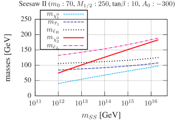
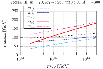
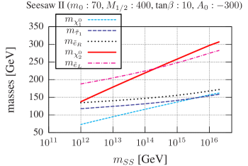
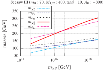
Figure 1: Supersymmetric masses for two specific choices of mSugra parameters as a function of the seesaw scale. To the left: type-II. To the right: type-III. The mSugra parameters are fixed at the values of SPS1a’ (top) and to MSP-1 (bottom). Note the different scales for type-II and type-III.

Fig. (1) shows some examples of SUSY masses for two specific choices of mSugra parameters. The top panel shows mSugra parameters chosen as in the standard point SPS1a’ AguilarSaavedra:2005pw , while the bottom panel shows MSP-1 for comparison. All plots show masses as function of $m_{SS}$, to the left for seesaw type-II and to the right for type-III. Shown are masses of the lighter two neutralinos, $\chi^{0}_{1}$ and $\chi^{0}_{2}$, and masses of charged sleptons. As is also typical in mSugra, the mass of the lighter chargino $m_{\chi^{+}_{1}}$ is very similar to $m_{\chi^{0}_{2}}$ and smuons and selectrons are nearly degenerate. We note in passing, that the mass of the lightest Higgs, $h^{0}$, shows little or no sensitivity at all on $m_{SS}$ but is important in the fits.

As discussed above, all masses get smaller for smaller values of $m_{SS}$ and are always smaller than in the pmSugra limit. Note the wide range for type-II shown and the much smaller range of $m_{SS}$ plotted for type-III. Ratios of gaugino masses follow standard expectations for all values of $m_{SS}$ and both types of seesaw. The slopes of the curves are different for different sparticles and the relative changes are larger in type-III than in type-II. This simply reflects the fact that type-III causes a larger change in the beta coefficients ($\Delta b_{i}=15$) than type-II ($\Delta b_{i}=7$).

For the point SPS1a’ the lighter chargino becomes lighter than 105 GeV for type-II (type-III) seesaw scales below roughly $m_{SS}\sim 2\times 10^{13}$ GeV ($m_{SS}\sim 10^{15}$ GeV). Thus, $m_{SS}$ below these values are ruled out by the LEP bounds Nakamura:2010zzi ; LEP2online . Note that this implies that type-III can not explain neutrino data for mSugra parameters as in SPS1a’ with Yukawas smaller than $Y_{W}^{ij}\leq 1$.

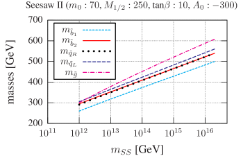
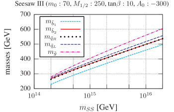
Figure 2: Running masses as a function of the seesaw scale, left: type-II; right: type-III. As fig. (1), but showing only the point SPS1a’. The masses shown in this figure are the most important coloured particles for our analysis.

Changing the seesaw scale can lead to a different mass ordering for different sparticles. For example, for SPS1a’ the $\chi^{0}_{2}$ is heavier than ${\tilde{e}}_{R}$ and ${\tilde{\tau}}_{1}$ in the mSugra limit (seesaw scale equal to $M_{G}$), but lighter than ${\tilde{e}}_{R}$ for type-II (type-III) seesaw scales below $m_{SS}\sim 3\times 10^{13}$ ($m_{SS}\sim 8\times 10^{14}$). This is important for our study, since as a function of $m_{SS}$ it can happen that some observables are kinematically open for some values of $m_{SS}$ but not for others, see also the discussion in section III.4.

The modified value of $M_{1/2}=400$ GeV in MSP-1 with respect to SPS1a’ is motivated by the fact that for this choice of parameters the edge variables from the chain $\chi^{0}_{2}\to{\tilde{l}}_{R}l\to ll\chi^{0}_{1}$ are kinematically possible for all relevant values of $m_{SS}$. The larger value of $M_{1/2}$ implies heavier neutralinos and also that the LEP bounds on sparticle masses are fulfilled for all values of $m_{SS}$ shown. Note, that all sparticles shown in the plot are kinematically accessible at an ILC with $\sqrt{s}=1$ TeV. For MSP-1 the lighter stau is the LSP for $m_{SS}$ larger than roughly $m_{SS}=10^{16}$ GeV. Thus, this point formally has no cosmologically acceptable pmSugra limit.

Fig. (2) shows the dependence of several coloured sparticle masses on $m_{SS}$. Again to the left (right) we show seesaw type-II (type-III). Note the different scales for type-II and type-III. We show only the values for SPS1a’ in this figure, masses for MSP-1 are larger but behave qualitatively very similar. The relative change of masses as a function of $m_{SS}$ is much larger than for the non-coloured sparticle masses shown in fig. (1). Here the range where $m_{\tilde{g}}\simeq m_{\tilde{q}_{L,R}}\raise 1.29167pt\hbox{$\;<$\kern-7.5pt\raise-4.73611pt\hbox{$\sim\;$}}300$ GeV is excluded by Tevatron data Nakamura:2010zzi ; TevatronBounds . However, this region is already excluded by LEP data. Note that $m_{\tilde{g}}>m_{{\tilde{b}}_{1}}$ for all values of $m_{SS}$ in this point. Coloured sparticle production gives the bulk of the SUSY cross section at the LHC as usual. In these points most of the coloured sparticles are not kinematically accessible at the ILC, except for low values of $m_{SS}$. Except $\tilde{t}_{1}$ we therefore do not take into account measurements of coloured sparticles at the ILC in our analysis, even though they could be potentially much more accurate than the corresponding measurements at the LHC.

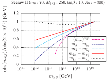
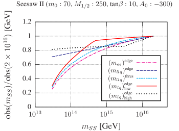
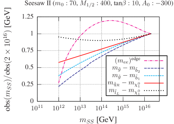
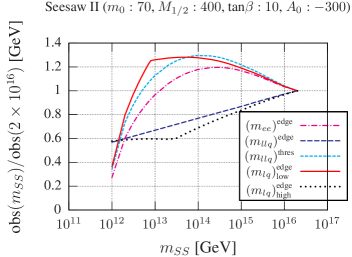
Figure 3: Relative change of different LHC observables as a function of the seesaw scale for type-II seesaw. Top mSugra parameters as in SPS1a’, bottom MSP-1. For an explanation see text. $(m_{ee})^{\rm edge}$ is repeated in the left plot for comparison.

With the masses shown in fig. (1) and fig. (2) one obtains the LHC observables shown in fig. (3) for type-II. Again in the top panel we show SPS1a’ and in the bottom panel MSP-1. The figure shows several mass differences (left) and the edge variables (right) stemming from the decay chain ${\tilde{q}}\to q\chi^{0}_{2}$ with the subsequent decay $\chi^{0}_{2}\to l^{\pm}{\tilde{l}}^{\mp}\to l^{\pm}l^{\mp}\chi^{0}_{1}$ Bachacou:1999zb ; Allanach:2000kt ; Lester:2001zx . We have normalized all observables to their expected values for $m_{SS}=M_{G}$. Thus relative changes in the different observables with respect to pmSugra are plotted.

The two kinks in the running of $(m_{lq})^{\text{edge}}_{\text{low}}$ and $(m_{lq})^{\text{edge}}_{\text{high}}$ stem from the fact that one has to consider different cases in these observables. They can be written as Allanach:2000kt

$$(m_{lq})^{\text{edge}}_{\text{high}} = \text{max}[(m_{l_{\text{near}}q}^{\text{max}})^{2},(m_{l_{\text{far}}q}^{\text{max}})^{2}]$$ (17)

$$(m_{lq})^{\text{edge}}_{\text{low}} = \text{min}[(m_{l_{\text{near}}q}^{\text{max}})^{2},(m_{\tilde{q}}^{2}-m_{\chi^{0}_{2}}^{2})(m_{\tilde{l}_{R}}^{2}-m_{\chi^{0}_{1}}^{2})/(2m_{\tilde{l}_{R}}^{2}-m_{\chi^{0}_{1}}^{2})]$$

where

$$(m_{l_{\text{near}}q}^{\text{max}})^{2} = (m_{\tilde{q}}^{2}-m_{\chi^{0}_{2}}^{2})(m_{\chi^{0}_{2}}^{2}-m_{\tilde{l}_{R}}^{2})/m_{\chi^{0}_{2}}^{2}$$ (18)

$$(m_{l_{\text{far}}q}^{\text{max}})^{2} = (m_{\tilde{q}}^{2}-m_{\chi^{0}_{2}}^{2})(m_{\tilde{l}_{R}}^{2}-m_{\chi^{0}_{1}}^{2})/(m_{\tilde{l}_{R}}^{2}).$$

These conditions change as a function of $m_{SS}$ causing the kinks shown in the figure. Except for the $(m_{ll})^{\rm edge}$ different cases appear in the expressions for all edges, but only for the variables $(m_{lq})^{\text{edge}}_{\text{low}}$ and $(m_{lq})^{\text{edge}}_{\text{high}}$ do the kinematical conditions change as function of $m_{SS}$ normally.

The plot in fig. (3) demonstrates the strong dependence of the LHC observables on $m_{SS}$. Increasing and decreasing values of the edges are possible, while mass differences usually decrease for lower values of $m_{SS}$. Note that in the $\chi^{2}$ fits, discussed in the next subsections, observables which show (a) the largest relative change with respect to $m_{SS}$ and (b) have the smallest expected errors will give the most important contributions. Finally we mention that fig. (3) shows only type-II, since results for type-III are qualitatively similar but with larger relative changes.

III.3 $\chi^{2}$ analysis for combined LHC and ILC data

In this section we take into account all possible LHC and ILC observables. We discuss this more futuristic (but simpler) case first. Results for an analysis taking only LHC observables are discussed in the next subsection. We note in passing that we have checked that we can roughly reproduce the error on parameters for the pure mSugra results for the point SPS1a’ discussed in detail in AguilarSaavedra:2005pw .

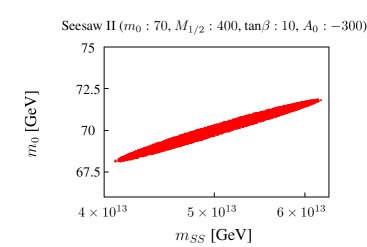
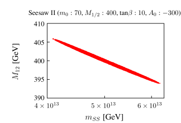
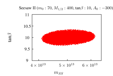
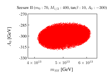
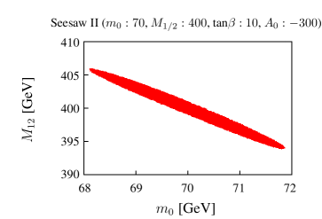
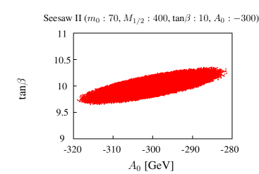
Figure 4: Allowed parameter space for $m_{0}$, $M_{1/2}$, $\tan\beta$, $A_{0}$ and $m_{SS}$ for all 5 parameters varied freely. The input value for the seesaw scale is $m_{SS}=5\times 10^{13}$ GeV and seesaw type-II has been used.

Fig. (4) shows the allowed ranges of the parameters for the point MSP-1 and one specific choice of $m_{SS}=5\times 10^{13}$ GeV for type-II seesaw. The allowed regions have been found in a MC random walk procedure letting 5 parameters, $m_{0},M_{1/2},A_{0},\tan\beta$ and $m_{SS}$, float freely. The ranges shown correspond to a $\Delta\chi^{2}\simeq 5.89$, i.e. 1 $\sigma$ c.l. for 5 free parameters, where we have taken into account the correlations between the various parameters. Plotted are different 2-dimensional projections of parameters.

As mentioned already above, the three parameters $m_{0}$, $M_{1/2}$ and $m_{SS}$ are highly correlated among each other. Lower values of $m_{SS}$ can be compensated by increasing $M_{1/2}$ and decreasing $m_{0}$ at the same time. This feature is present in all parameter space for both types of seesaw. This correlation results in errors on $m_{0}$ and $M_{1/2}$ which are larger (some times much larger, see below) than in pmSugra for the same input errors on observables. We note that the $\chi^{2}$ in this calculation is dominated by the much more accurate ILC data, see also the discussion in section (III.5) below.

In contrast, $\tan\beta$ and $A_{0}$ show very little correlation with $m_{SS}$ (and $m_{0}$ and $M_{1/2}$) and only a rather moderate correlation among themselves. $\tan\beta$ and $A_{0}$ are mostly determined by the Higgs mass measurement, and to some extend by 3rd generation sfermions. Note that $A_{0}$ and $\tan\beta$ do not have much influence on the determination of $m_{0}$, $M_{1/2}$ and $m_{SS}$, apart from a slight increase in the errors of the latter. However if $m_{0}$ cannot be fixed a determination of $A_{0}$ and also $\tan\beta$ becomes practically impossible, because almost any shift of $\tan\beta$ and $A_{0}$ can then be compensated by changing $m_{0}$ and/or $M_{1/2}$. This will be important when we discuss the calculations using LHC observables only in section III.4.

For this choice of parameters, the error on $m_{SS}$ itself is found to be around $\Delta m_{SS}\sim 1.2\times 10^{13}$, i.e. values of $m_{SS}=M_{G}$ are formally excluded by many standard deviations. However, $\Delta m_{SS}$ is a very strong function of $m_{SS}$ itself, as we will discuss below.

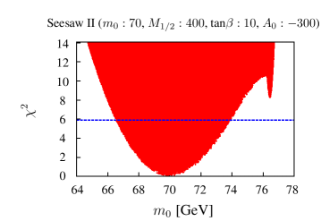
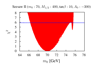
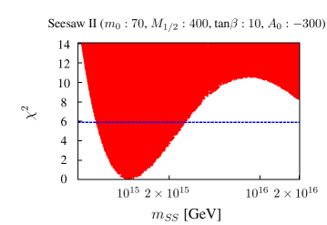
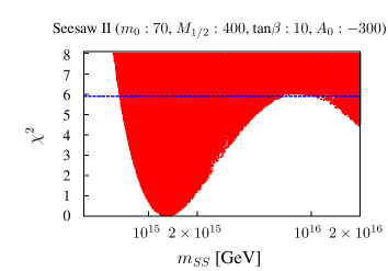
Figure 5: $\chi^{2}$ distributions of the random walk for MSP-1 and Seesaw type II. The dashed line indicates a $\chi^{2}$ of $5.89$. Recall that $5.89$ corresponds to a $1\sigma$ confidence level for five free parameters. The plots show the $\chi^{2}$ distributions for $m_{SS}=1\times 10^{15}$ GeV (left) and $m_{SS}=1.3\times 10^{15}$ GeV (right).

Fig. (4) shows results for a comparatively low value of $m_{SS}$. Fig. (5) shows $\chi^{2}$ distributions for MSP-1 obtained by a random walk for seesaw type II and two slightly different but much higher values of $m_{SS}$: To the left: $m_{SS}=10^{15}$ GeV and to the right: $m_{SS}=1.3\times 10^{15}$. The plots show the true $\chi^{2}$-minimum and a second (fake) minimum at $m_{SS}=M_{G}$. For the lower value of $m_{SS}$ this fake minimum is just excluded at 1 $\sigma$ c.l., while for the slightly higher value of $m_{SS}$ it is accepted at 1 $\sigma$ c.l. These kind of false minima appear in all our calculations when $m_{SS}$ approaches $M_{G}$. This is to be expected, since the models approach pmSugra in this limit.

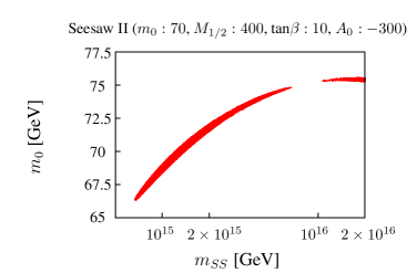
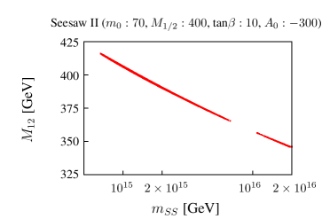
Figure 6: Allowed ranges of parameters $m_{SS}$, $m_{0}$ and $M_{1/2}$ for MSP-1 and type-II seesaw with input $m_{SS}=1.3\times 10^{15}$ GeV. Two separate solutions appear, one fake but acceptable minimum is at $m_{SS}=M_{G}$.

Fig. (6) shows the allowed range of parameters $m_{SS}$, $m_{0}$ and $M_{1/2}$ for $m_{SS}=1.3\times 10^{15}$ GeV. Two separate minima show up. For slightly larger values of $m_{SS}$ the two solutions overlap completely. Note that this also increases the errors on $m_{0}$ and $M_{1/2}$. For slightly smaller values of $m_{SS}$ this fake solution disappears resulting in a drastic decrease in the error bars of these three parameters. In case of type-III this fake minima does not show up separately, but indirectly by deforming the $\chi^{2}$ distributions. Thus for type-III the error bars go up to $M_{G}$ until it gets compatible with pmSUGRA. This will be important when we discuss mSUGRA plus type-III later on.

In case of the ILC+LHC analysis this kind of “false” minima are usually the only class of fake minima that appear. Using only LHC data, the $\chi^{2}$ distributions are not that well behaved and false minima can also appear considerably below $M_{G}$, this will be shown in the next subsection.

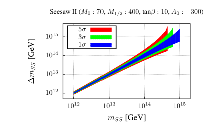
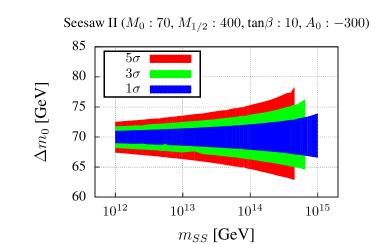
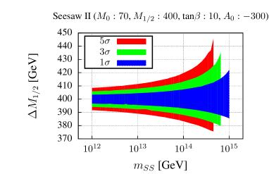
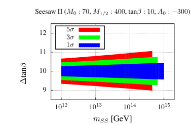
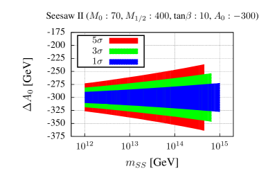
Figure 7: Error of $m_{SS}$, $m_{0}$, $M_{1/2}$, $tan\beta$ and $A_{0}$ against $m_{SS}$ for all 5 parameters freely varied. For these plots we used the LHC and ILC observables. The chosen values for $m_{SS}$, $m_{0}$, $M_{1/2}$, $tan\beta$ and $A_{0}$ are the values for MSP-1. The plots show the results for seesaw type II where we used a $1\sigma$, $3\sigma$ and $5\sigma$ c.l..

Fig. (7) shows 1 $\sigma$, 3 $\sigma$ and 5 $\sigma$ c.l. error bars on the different parameters of the model as a function of the seesaw scale for one specific mSugra set, MSP-1, for the case of type-II. The plots show a large range of $m_{SS}$ between [$10^{12},10^{15}$] GeV. Lower values of $m_{SS}$ are in principle possible, but show no new features. Larger values of $m_{SS}$ can not fit current neutrino data. Error bars on all parameters increase with increasing values of $m_{SS}$, and for values of $m_{SS}$ larger than (roughly) $(1-2)\times 10^{15}$ GeV the error $\Delta(m_{SS})$ is so large that the type-II can no longer be distinguished from pmSugra at the 1-$\sigma$ level, given the ILC+LHC observables with our “standard” errors. $\Delta(m_{SS})$ decreases very rapidly as a function of $m_{SS}$ and for values of $m_{SS}=6.5\times 10^{14}$ ($4.5\times 10^{14}$) pmSugra and type-II can be formally distinguished by more than 3 (5) standard deviations.

Also the errors $\Delta(m_{0})$ and $\Delta(M_{1/2})$ do show dependence on $m_{SS}$, especially at larger values of $m_{SS}$. Again, the reason for this dependence is found in the strong correlation among those three parameters, as discussed above. The error $\Delta(\tan\beta)$ (and to some extend $\Delta(A_{0})$), on the other hand, shows less dependence on $m_{SS}$. This is explained by the fact that the lightest Higgs mass, $m_{h^{0}}$, shows very little dependence on the seesaw scale. The slight dependence of $\Delta(A_{0})$ on $m_{SS}$ is due to the lightest stop mass. For simplicity in all following plots we show only the 1 $\sigma$ allowed regions.

Figure 8: Error of $m_{SS}$, against $m_{SS}$ for 5 free parameters. For these plots we used the LHC and ILC observables. The chosen values of parameters correspond to MSP-2 (left) and MSP-3 (right). The plots show the results for Seesaw type-II.

Fig. ( 8) shows two more examples of $\Delta(m_{SS})$ as a function of $m_{SS}$. Here results for the points MSP-2 and MSP-3 are shown for type-II seesaw. Only $\Delta(m_{SS})$ as a function of $m_{SS}$ is shown. We do not repeat the plots for the other parameters because they are qualitatively very similar to the case shown in fig. (7). As the plots show results for MSP-2 and MSP-3 are similar to MSP-1. Values of $m_{SS}$ below roughly $m_{SS}\sim 10^{15}$ GeV are inconsistent with pmSugra. This implies that for the ILC errors as estimated in Weiglein:2004hn and AguilarSaavedra:2005pw a combined ILC+LHC analysis should be able to distinguish pmSugra from type-II seesaw for nearly all values of $m_{SS}$ relevant for neutrino data. We stress that this conclusion is correct only for those mSugra parameters for which (both left- and right-) sleptons and the lightest neutralino are kinematically accessible at the ILC.

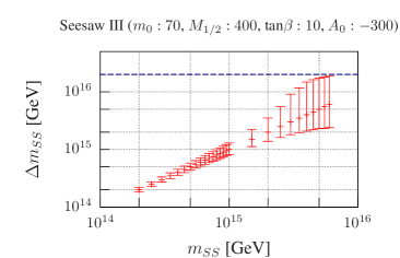
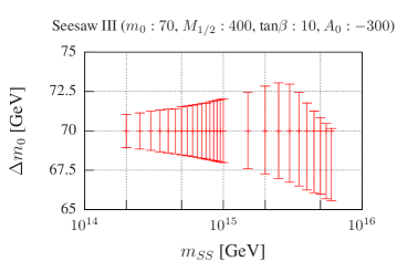
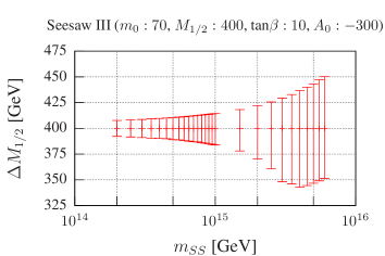
Figure 9: Error of $m_{SS}$, $m_{0}$ and $M_{1/2}$ against $m_{SS}$ for 5 parameters varied freely. For these plots we used the LHC and ILC observables. The chosen values for $m_{SS}$, $m_{0}$, $M_{1/2}$, $tan\beta$ and $A_{0}$ are the values according to MSP-1. The plots show the results for seesaw type III.

Up to now we have shown only results for seesaw type-II. Fig. (9) shows a corresponding calculation for type-III and mSugra parameters as in MSP-1. Again, MSP-2 and MSP-3 show similar behaviour and we do not repeat the plots for these points. Again, the scale of $m_{SS}$ is different from the case of type-II. Since SUSY masses show a stronger dependence on $m_{SS}$ in type-III than in type-II, larger values of $m_{SS}$ can be distinguished from pmSugra in this case. In the examples shown in the figure all values of $m_{SS}$ below roughly $m_{SS}\sim 5-6\times 10^{15}$ GeV can be distinguished from pmSugra with more than 1 $\sigma$ c.l. Recall that in type-III one expects $m_{SS}\raise 1.29167pt\hbox{$\;<$\kern-7.5pt\raise-4.73611pt\hbox{$\sim\;$}}8\times 10^{14}$ in order to explain neutrino data. Such “low” values of $m_{SS}$ differ from pmSugra in the fits by many standard deviations.

Errors on $m_{0}$ are similar to the values observed for type-II, while $\Delta(M_{1/2})$ is larger in type-III. The correlation between $m_{0}$, $M_{1/2}$ and $m_{SS}$, discussed above for type-II, is also present in type-III and with an even larger correlation between $M_{1/2}$ and $m_{SS}$ in this case. The mSUGRA solution does not show up explicitly as a second separate minimum, but deforms the $\chi^{2}$ distributions, thus cutting the allowed ranges of $m_{0}$ and $M_{1/2}$.

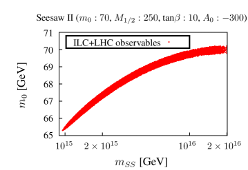
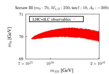
Figure 10: The plots show random walks in which as starting point SPS1a’ was chosen. For the parameter fit we used mSUGRA plus seesaw type-II and III, respectively. The runs take into account LHC and ILC observables.

Up to now we have always used a seesaw spectrum as input. One can also ask the opposite question: Can a pmSugra point mimic a seesaw spectrum? An example of such a calculation is shown in fig. (10). In this figure we show the allowed ranges for $m_{SS}$ and $m_{0}$ for mSugra parameters as in SPS1a’ for type-II (left) and type-III (right). As one can see $m_{SS}$ as low as $m_{SS}\sim 10^{15}$ GeV ($m_{SS}\sim 7\times 10^{15}$ GeV) are allowed at 1 $\sigma$ c.l. for type-II (type-III) fits. Also note that $\Delta(m_{0})$ is much larger than in a pmSugra fit, due again to the observed correlation among parameters. The results shown in fig. (10) are consistent with the results discussed above, when a seesaw spectrum is used as input: $m_{SS}$ compatible with $M_{G}$ is reached at a very similar value of $m_{SS}$.

Finally we note, that distinguishing type-II from type-III requires extremely high precision, since they differ only at 2-loop order. The reason is that for 1-loop RGEs one can always cancel the shifts in the coefficient of the beta-functions by a rescaling of $m_{SS}$. We have checked this numerically.

Closing this section we note that all results shown above have been obtained for the full 2-loop calculation. We have repeated the exercise in several cases using 1-loop RGEs only. As a general result, due to the weaker running of 1-loop RGEs, differences between pmSugra and seesaw are slightly smaller, leading to slightly larger errors on the parameters. For the case of the ILC+LHC analysis, however, differences between both calculations are rather small, with errors in parameters typically increasing in the order of (10-30) % when going from a 2-loop to a 1-loop calculation.

III.4 LHC only

In this subsection we discuss the results for an analysis using only LHC measurements. At the LHC observables do not measure SUSY masses directly. Instead, observables measure either mass differences or, in case of the edge variables, combinations of mass squared differences. Also one expects that LHC measurements will be much less precise than what can be done in case of the ILC. As a result the $\chi^{2}$ distributions for an LHC-only analysis show more complicated features than for the case of LHC+ILC. Especially it should be noted that in some cases we do not have a sufficiently large number of well determined observables and fake minima can appear, which will lead to sometimes rather large error bars on parameters, as discussed below.

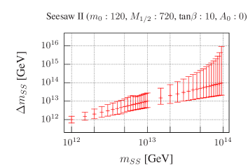
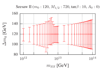
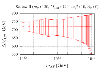
Figure 11: Error of $m_{SS}$, $m_{0}$, $M_{1/2}$, $tan\beta$ and $A_{0}$ against $m_{SS}$ for $m_{SS}$, $m_{0}$, $M_{1/2}$, $tan\beta$ and $A_{0}$ varied. For these plots we used only the LHC observables. The chosen values for $m_{SS}$, $m_{0}$, $M_{1/2}$, $tan\beta$ and $A_{0}$ are the values according to MSP-3. The plots show the results for seesaw type II.

Fig. (11) shows error bars on $m_{SS}$, $m_{0}$, $M_{1/2}$ against $m_{SS}$ for the point MSP-3 and seesaw type-II, again for all 5 parameters varied freely. Note the change in the scale for $m_{SS}$, the largest value shown is $m_{SS}=10^{14}$ GeV. For larger values of $m_{SS}$ type-II seesaw can no longer be distinguished in this fit from pmSugra with at least 1 $\sigma$ c.l. Note, however, that $\Delta(m_{SS})$ decreases very rapidly for decreasing values of $m_{SS}$ and for values of $m_{SS}$ below $m_{SS}\sim$ (few) $10^{13}$ GeV pmSugra and type-II are formally different by several standard deviations.

The figure shows also that $\Delta(m_{0})$ and $\Delta(M_{1/2})$ are much larger for the case of using only LHC observables than in the combined ILC+LHC analysis, as expected. Errors on $m_{0}$ and $M_{1/2}$ decrease in general with decreasing $m_{SS}$. The increase in $\Delta(m_{0})$ and $\Delta(M_{1/2})$ around $m_{SS}\sim 7\times 10^{12}$ GeV is due to the appearance of a fake side-minimum. Such fake minima appear only for certain ranges of $m_{SS}$. Depending on which side of the real minimum they appear they can lead to an asymmetric increase of the errors as observed in this figure.

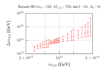
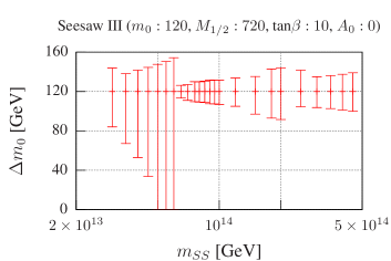
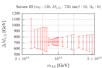
Figure 12: Error of $m_{SS}$, $m_{0}$, $M_{1/2}$ against $m_{SS}$ for 5 parameters varied freely. For these plots we used only the LHC observables. The chosen values for $m_{SS}$, $m_{0}$, $M_{1/2}$, $tan\beta$ and $A_{0}$ are the values according to MSP-3. The plots show the results for seesaw type III.

Fig. (12) shows an example of a corresponding fit for type-III. Again, $\Delta(m_{0})$ and $\Delta(M_{1/2})$ and $\Delta(m_{SS})$ are shown as a function of $m_{SS}$ for MSP-3. Note that other points show qualitatively similar behaviour and that the range shown for $m_{SS}$ is comparatively small. Values of $m_{SS}$ larger than $m_{SS}\sim 5\times 10^{14}$ are 1 $\sigma$ c.l. consistent with pmSugra. Since $m_{SS}\raise 1.29167pt\hbox{$\;<$\kern-7.5pt\raise-4.73611pt\hbox{$\sim\;$}}8\times 10^{14}$ to explain neutrino data, LHC-only can probe interesting parts of the parameter space, but certainly will not be able to cover all possible values of $m_{SS}$ - unless LHC errors on mass measurements can be improved compared to expectations by considerable factors.

For decreasing $m_{SS}$ errors again decrease in general. There are two exceptions from this general rule in this plot. First, errors increase around $m_{SS}\sim 2\times 10^{14}$ GeV. This is again due to the appearance of a fake side minimum, which slowly disappears again when going towards smaller values of $m_{SS}$. The large increase in the error bars around $m_{SS}\sim 6\times 10^{13}$ GeV is due to the fact that for smaller values of $m_{SS}$ in this calculation $\chi^{0}_{2}$ is lighter than ${\tilde{e}}_{R}$, i.e. the edges variables are lost completely. With only a few observables in the fit, all based on mass differences, $m_{0}$ and $M_{1/2}$ can hardly be fixed at all. The dramatic increase of the error bars of $m_{0}$ can be understood easily from Eq. (15). As this equation shows the sfermion masses behave approximately like $m_{\tilde{f}}^{2}=m_{0}^{2}+aM_{1/2}^{2}$. When all edges are lost the remaining LHC observables can be fitted by varying $m_{SS}$ and $M_{1/2}$ only.

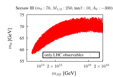
Figure 13: The plots show the result of a random walk in which as a starting point SPS1a’ was chosen. For the parameter fit we used mSUGRA plus seesaw type II and III, respectively. The runs were made for LHC observables enabled only.

Finally we have calculated the allowed parameter space in a seesaw fit when the true input point is pmSugra. Two examples are shown in Fig. (13). The mSugra parameters are for SPS1a’ and type-II (type-III) seesaw is shown to the left (right). The allowed regions are much larger than in the combined ILC+LHC analysis, compared to the discussion in the last subsections. For type-II (type-III) values of $m_{SS}$ as low as $m_{SS}\raise 1.29167pt\hbox{$\;<$\kern-7.5pt\raise-4.73611pt\hbox{$\sim\;$}}10^{14}$ GeV ($m_{SS}\raise 1.29167pt\hbox{$\;<$\kern-7.5pt\raise-4.73611pt\hbox{$\sim\;$}}6\times 10^{14}$ GeV) are allowed at the 1 $\sigma$ level. This is similar - and consistent - with the results discussed above for the opposite fit.

In summary mass measurements from the LHC only should be able to distinguish between pmSugra and type-II (type-III) seesaw for seesaw scales below roughly $m_{SS}\raise 1.29167pt\hbox{$\;<$\kern-7.5pt\raise-4.73611pt\hbox{$\sim\;$}}10^{14}$ GeV ($m_{SS}\raise 1.29167pt\hbox{$\;<$\kern-7.5pt\raise-4.73611pt\hbox{$\sim\;$}}6\times 10^{14}$ GeV). This conclusion depends critically on the possibility to measure accurately several observables, as we are going to discuss next.

III.5 Required accuracies on mass measurements and $\Delta(m_{SS})$

All our results shown above crucially depend on the size of the expected error bars for the different observables. In this section we therefore discuss in some detail: (a) Which are the most important observables in our fits? And, (b) How accurately do we need to measure them to distinguish pmSugra from seesaw for a given, fixed value of $m_{SS}$. Again we will discuss the ILC+LHC case first.

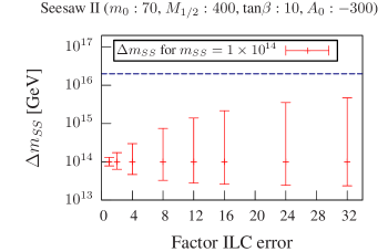
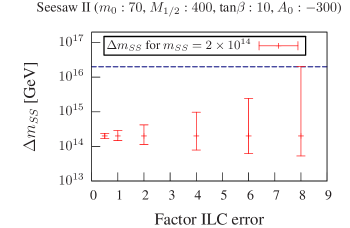
Figure 14: Error of $m_{SS}$ with respect to the error of the ILC observables, $f_{ILC}$.

Fig. (14) shows $\Delta(m_{SS})$ for the points MSP-1 for two choices of $m_{SS}$. $\Delta(m_{SS})$ is shown as a function of the error of the ILC mass measurements. According to AguilarSaavedra:2005pw it is expected that the ILC can measure SUSY masses of $\chi^{0}_{i}$ and ${\tilde{l}}$ states kinematically accessible with errors of the order (0.5-2) per-mille. We define a common factor $f_{ILC}$ and multiply all relative errors given in table 6 of AguilarSaavedra:2005pw with this common factor. $\Delta(m_{SS})$ is then shown as a function of this factor in fig. (14). Note that in this calculation we keep all LHC errors unchanged at their “standard values”.

As fig. (14) to the left shows, $\Delta(m_{SS})$ increases with the assumed errors of the ILC measurements. However, for MSP-1 and $m_{SS}=10^{14}$ GeV, LHC measurements alone are sufficient to distinguish type-II from pmSugra. Thus, error bars on $m_{SS}$ hardly increase going from $f_{ILC}=24$ to $f_{ILC}=32$. This means that ILC data dominate the fit until errors are about one order of magnitude larger than estimated in AguilarSaavedra:2005pw , for larger ILC errors LHC measurements become more important for this choice of $m_{SS}$.

The situation is quite different for $m_{SS}=2\times 10^{14}$ GeV, see fig. (14) right. While $f_{ILC}=6$ still allows to distinguish between pmSugra and type-II, for $f_{ILC}=8$, $\Delta(m_{SS})$ becomes to large to differentiate between type-II and pmSugra. The required accuracy of measurements of SUSY masses at the ILC is therefore a strong function of $m_{SS}$ itself. Errors of the order (1-2) percent are in general tolerable for seesaw scales below $m_{SS}=10^{14}$ GeV, while per-mille level measurements are required in the interval $[10^{14},10^{15}]$ GeV. We note that other SUSY points behave very similar and that for type-III correspondingly larger errors are tolerable.

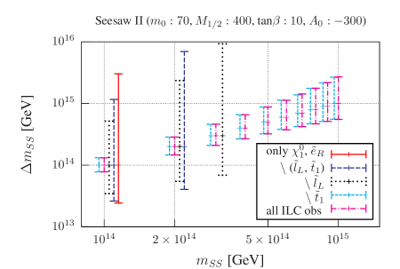
Figure 15: In this plot the errors of $m_{SS}$ with respect to $m_{SS}$ are shown. The different lines belong to different runs where different combinations of ILC observables were switched off. The different lines belong in each case to the same $m_{SS}$ values but were a bit to be able to distinguish them. The real $m_{SS}$ value is the value of the pink error bars which correspond to the run for all ILC observables enabled.

Fig. (14) treats all ILC observables equally. An interesting question to ask is, of course, which ILC observables are the most important ones for our analysis. Fig. (15) provides the answer. Again for the point MSP-1 and for seesaw type-II we show $\Delta(m_{SS})$ as a function of $m_{SS}$ for different calculations taking into account different observables. We have kept all LHC observables “on” at their standard errors. “All ILC obs” is the standard fit, taking into account all kinematically accessible mass measurements with their original errors from AguilarSaavedra:2005pw . We then switched off by hand completely the contributions from different observables. Switching off the measurement of the mass of ${\tilde{t}}_{1}$ hardly changes the result. On the other hand, it can be seen that measuring left-slepton masses is highly important. Error bars increase sizeably if this observable is not taken into account and while a set of measurements with all observables can distinguish pmSugra from type-II all the way up to $m_{SS}=10^{15}$ GeV, without the accurate measurement of $m_{{\tilde{l}}_{L}}$ all values of $m_{SS}\raise 1.29167pt\hbox{$\;>$\kern-7.5pt\raise-4.73611pt\hbox{$\sim\;$}}4\times 10^{14}$ GeV are compatible with pmSugra at the 1 $\sigma$ level. The relative importance of ${\tilde{l}}_{L}$ despite its larger error stems from the fact that $m_{{\tilde{l}}_{R}}$ has very little sensitivity to $m_{SS}$, see fig. (1).

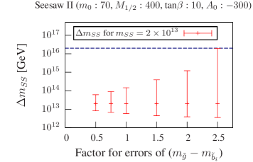
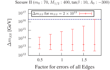
Figure 16: Error of $m_{SS}$ with respect to the error of $(m_{\tilde{g}}-m_{\tilde{b}_{1}})$ and $(m_{ll})^{\text{edge}}$. According to Weiglein:2004hn the error on $(m_{\tilde{g}}-m_{\tilde{b}_{1}})$ is expected to be $\sim 3.5\%$ and the error of $(m_{ll})^{\text{edge}}$ is estimated as $\sim 0.17\%$. Note that we also changed the error of $(m_{\tilde{g}}-m_{\tilde{b}_{2}})$, accordingly.

We now turn to the discussion of LHC errors. In this case we do not use any input from the ILC. Fig. (16) shows $\Delta(m_{SS})$ as a function of the assumed error. Two observables are shown: to the left as a function of $\Delta_{{\tilde{g}}{\tilde{b}}_{i}}$ and to the right as a function of the edge variables. Note that for SPS1a the LHC error for $\Delta_{{\tilde{g}}{\tilde{b}}_{1}}$ is estimated to be $\sim 3.5$ %, while $\Delta(m_{ll}^{\text{edge}})$ should be measured to an accuracy of $0.17$ %. Note that, while $\Delta(m_{ll}^{\text{edge}})$ can possibly be accurately measured in wide ranges of mSugra parameter space, the accuracy with which $\Delta_{{\tilde{g}}{\tilde{b}}_{i}}$ can be measured is far less certain. Both smaller and much larger errors on this quantity have been found in different study points, see Weiglein:2004hn .

The figure shows that for $m_{SS}=2\times 10^{13}$ a $7$ % error on $\Delta_{{\tilde{g}}{\tilde{b}}_{1}}$ (which corresponds to a factor of 2 in the plot) is sufficient to distinguish between pmSugra and type-II, while an error of $9$ % on this quantity is not sufficient. Again, the maximum value of this error which still allows to distinguish between type-II and pmSugra is a strong function of the (unknown) $m_{SS}$ itself. However, we have found that always $\Delta_{{\tilde{g}}{\tilde{b}}_{1}}$ is a critical input observable for our analysis. The importance of $\Delta_{{\tilde{g}}{\tilde{b}}_{1}}$ can be understood from Fig. (2) and (3): coloured sparticle masses depend much more strongly on $m_{SS}$ than masses of, for example, sleptons. Thus, despite the larger relative error on $\Delta_{{\tilde{g}}{\tilde{b}}_{1}}$ compared to the edge variables,it is nearly as important as demonstrated in fig. (16) to the right.

Fig. (17) shows the results of different runs, where we have switched off artificially different combinations of observables. As noted above, $\Delta_{{\tilde{g}}{\tilde{b}}_{1}}$ and the edges are the most important observables for fixing $\Delta(m_{SS})$. However, the Higgs mass measurement is not negligible, despite the fact that $\Delta(m_{SS})$ does not increase much in the figure, when $m_{h^{0}}$ is switched off. This importance lies in the fact that without $m_{h^{0}}$ the largest value of $m_{SS}$ not compatible with $M_{G}$ is $2\times 10^{13}$ GeV, compared to $m_{SS}=10^{14}$ GeV for $m_{h^{0}}$ switched on.

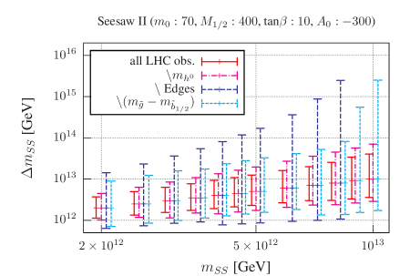
Figure 17: In this plot the errors of $m_{SS}$ with respect to $m_{SS}$ are shown. The different lines belong to different runs at which we switched off different combinations of LHC observables. The different lines belong in each case to the same $m_{SS}$ values but we separated them in the plot a bit to be able to distinguish them. The real $m_{SS}$ value is the value of the pink error bars that correspond to the run in which the Higgs mass measurement is disabled.

We do not repeat the discussion for type-III seesaw. Results are very similar qualitatively, but again larger values of $m_{SS}$ can be tested for the same errors on the observables.

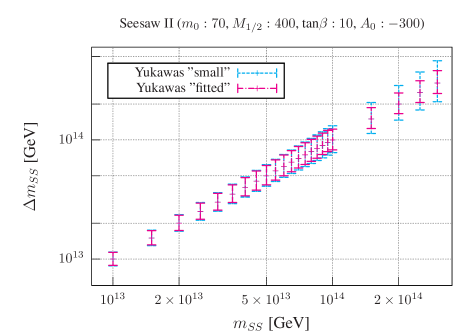
Figure 18: In this plot the errors of $m_{SS}$ with respect to $m_{SS}$ are shown. The different lines belong to two different runs at which we set the Yukawa couplings to very small values ($\sim 10^{-4}$) in the first run and in the second one we fitted the Yukawa couplings to neutrino data and calculated the error with the fitted values.

Finally, we turn to the question of Yukawa couplings. Fig. (18) shows again $\Delta(m_{SS})$ as a function of $m_{SS}$ for two different calculations: (i) a calculation with triplet Yukawa couplings negligibly small (all $(Y_{T})_{ij}\sim{\cal O}(10^{-4})$) and (ii) a calculation in which $Y_{T}$ has been fitted to give the atmospheric and solar neutrino mass squareds at their best fit values with neutrino angles taking tri-bimaximal values. As can be seen, differences between both calculations become negligible below roughly $m_{SS}=10^{14}$ GeV, as expected. For larger values of $m_{SS}$ correctly fitting the Yukawas leads to slightly smaller errors on $m_{SS}$. This can be understood, since for finite Yukawas SUSY masses change slightly stronger than for infinitesimal values of $Y_{T}$, making the fit easier. Note, however, that we have not scanned over all allowed range of $Y_{T}$ in this calculation. In a complete $14$ parameter $\chi^{2}$ fit errors might be larger. Note also, we can not find any good neutrino solution for $m_{SS}$ larger than $m_{SS}=6\times 10^{14}$, since in this calculation we have chosen for the coupling $\lambda_{2}=0.5$. In conclusion, a full fit including Yukawa couplings will be necessary only if signs of $m_{SS}\raise 1.29167pt\hbox{$\;>$\kern-7.5pt\raise-4.73611pt\hbox{$\sim\;$}}10^{14}$ GeV have been found in SUSY mass data.

IV Conclusions and discussion

We have studied the possibility to obtain indirect information on the seesaw scale from SUSY mass measurements at future colliders. Since in the type-I seesaw only SM singlets are added to the MSSM particle content, none of the measurements which we considered are expected to show sizeable departures from mSugra expectations. We therefore concentrated on the type-II and type-III realizations of the seesaw.

Assuming mSugra boundary conditions and taking error estimates as forecasted by study groups we find that a combination of LHC and ILC measurements should be able to distinguish pure mSugra from mSugra plus either type-II or type-III seesaw for nearly any relevant values of the seesaw scale, if (a) at least $\chi^{0}_{1}$, ${\tilde{e}}_{R}$/ ${\tilde{\mu}}_{R}$ and ${\tilde{e}}_{L}$/ ${\tilde{\mu}}_{L}$ are kinemetically accessible at the ILC and (b) the LHC can measure $m_{\tilde{g}}-m_{{\tilde{b}}_{1}}$ and the edge observables accurately. We always assume that the lightest Higgs has been found. The degree of confidence with which pmSugra can be distinguished from mSugra plus seesaw depends sensitively on the actual value of the seesaw scale. At the “critical” value of $m_{SS}\sim 10^{15}$, beyond which neutrino data can no longer be explained with Yukawas smaller than 1, the difference between type-II + mSugra and pmSugra could be as low as only 1 $\sigma$ c.l. However, the difference between pmSugra and mSugra + seesaw rises very sharply with decreasing $m_{SS}$ and formally more than 5 $\sigma$ c.l. could be reached already at $(5-6)\times 10^{14}$ for type-II. Differences between pmSugra and mSugra plus type-III are always found to be larger than for mSugra plus type-II for the same value of $m_{SS}$.

As expected, the future is not as bright, if we take into account only LHC data. Nevertheless, using only LHC data one can distinguish pure mSugra and mSugra plus seesaw in some favourable parts of parameter space. Especially, we point out that the lower the real value of the seesaw scale $m_{SS}$ is, the easier it becomes to distinguish pure mSugra from mSugra plus seesaw. We have discussed the most important measurements for the LHC and the ILC and the relative errors with which these observables need to be measured for this analysis to be possible. In our analysis we used exclusively mSugra SUSY breaking boundary conditions, but other, more involved SUSY breaking schemes with more free parameters could, in principle, be “tested” in a similar way.

Of course, the analysis presented in this paper is far from being complete. If SUSY is found at the LHC, one would need to redo our calculations with real data. However, the experimentalist would not, as we have always assumed in our fits, know the real values of the parameters. We have tried for a few points, whether the correct input parameters can be retrieved for arbitrary starting points in our MC random walk procedure and - given enough CPU-time - are able to find the correct minimum. However, our “observables” are theoretically calculated observables and thus perfect in contrast to real data which are expected to scatter around the true values and might show tension between different observables. Thus, finding the correct minimum in real data might be more difficult. Moreover, the underlying model will not be known a priori and, thus, $\chi^{2}_{Min}$ for different models need to be calculated and compared.

Nevertheless, even taking into account the limitations of our study, we think it is highly motivating that type-II and type-III seesaw leave sizeable traces in SUSY spectra, which should show up, if sufficiently accurate mass measurements are possible and become available.

References

- (1) A. H. Chamseddine, R. L. Arnowitt and P. Nath, Phys. Rev. Lett. 49 (1982) 970.
- (2) H. P. Nilles, Phys. Rept. 110 (1984) 1.
- (3) G. F. Giudice, M. A. Luty, H. Murayama and R. Rattazzi, JHEP 9812 (1998) 027 [arXiv:hep-ph/9810442].
- (4) Z. Chacko, M. A. Luty, I. Maksymyk and E. Ponton, JHEP 0004 (2000) 001 [arXiv:hep-ph/9905390].
- (5) For a review on GMSB, see: G. F. Giudice and R. Rattazzi, Phys. Rept. 322 (1999) 419 [arXiv:hep-ph/9801271].
- (6) J. A. Aguilar-Saavedra et al. [ECFA/DESY LC Physics Working Group], arXiv:hep-ph/0106315.
- (7) G. Weiglein et al. [LHC/LC Study Group], Phys. Rept. 426 (2006) 47 [arXiv:hep-ph/0410364].
- (8) J. A. Aguilar-Saavedra et al., Eur. Phys. J. C 46, 43 (2006) [arXiv:hep-ph/0511344].
- (9) G. A. Blair, W. Porod and P. M. Zerwas, Phys. Rev. D 63 (2001) 017703 [arXiv:hep-ph/0007107].
- (10) G. A. Blair, W. Porod and P. M. Zerwas, Eur. Phys. J. C27, 263 (2003), [hep-ph/0210058].
- (11) P. Bechtle, K. Desch, W. Porod and P. Wienemann, Eur. Phys. J. C 46 (2006) 533 [arXiv:hep-ph/0511006].
- (12) R. Lafaye, T. Plehn, M. Rauch and D. Zerwas, Eur. Phys. J. C 54 (2008) 617 [arXiv:0709.3985 [hep-ph]].
- (13) C. Adam, J. L. Kneur, R. Lafaye, T. Plehn, M. Rauch and D. Zerwas, arXiv:1007.2190 [hep-ph].
- (14) Y. Fukuda et al. [Super-Kamiokande Collaboration], Phys. Rev. Lett. 81, 1562 (1998)
- (15) SNO, Q. R. Ahmad et al., Phys. Rev. Lett. 89, 011301 (2002), [nucl-ex/0204008].
- (16) KamLAND, K. Eguchi et al., Phys. Rev. Lett. 90, 021802 (2003), [hep-ex/0212021].
- (17) KamLAND Collaboration, arXiv:0801.4589 [hep-ex].
- (18) For a recent review on the status of neutrino oscillation data, see: T. Schwetz, M. A. Tortola and J. W. F. Valle, New J. Phys. 10, 113011 (2008) [arXiv:0808.2016 [hep-ph]]. Version 3 on the arXive is updated with data until Feb 2010
- (19) P. Minkowski, Phys. Lett. B 67 (1977) 421.
- (20) T. Yanagida, in KEK lectures, ed. O. Sawada and A. Sugamoto, KEK, 1979; M Gell-Mann, P Ramond, R. Slansky, in Supergravity, ed. P. van Niewenhuizen and D. Freedman (North Holland, 1979);
- (21) R.N. Mohapatra and G. Senjanovic, Phys. Rev. Lett. 44 912 (1980).
- (22) E. Ma, Phys. Rev. Lett. 81, 1171 (1998) [arXiv:hep-ph/9805219].
- (23) J. Schechter and J. W. F. Valle, Phys. Rev. D 22, 2227 (1980).
- (24) T. P. Cheng and L. F. Li, Phys. Rev. D 22, 2860 (1980).
- (25) R. Foot, H. Lew, X. G. He and G. C. Joshi, Z. Phys. C 44, 441 (1989).
- (26) A rather incomplete list on LFV in SUSY seesaw, mainly on type-I is: J. Hisano, T. Moroi, K. Tobe and M. Yamaguchi, Phys. Rev. D53, 2442 (1996); J. R. Ellis, J. Hisano, M. Raidal and Y. Shimizu, Phys. Rev. D 66, 115013 (2002); F. Deppisch, H. Paes, A. Redelbach, R. Rückl and Y. Shimizu, Eur. Phys. J. C28, 365 (2003); S. T. Petcov, S. Profumo, Y. Takanishi and C. E. Yaguna, Nucl. Phys. B 676 (2004) 453; E. Arganda and M. J. Herrero, Phys. Rev. D73, 055003 (2006); S. T. Petcov, T. Shindou and Y. Takanishi, Nucl. Phys. B 738, 219 (2006); S. Antusch, E. Arganda, M. J. Herrero and A. M. Teixeira, JHEP 11, 090 (2006); F. Deppisch and J. W. F. Valle, Phys. Rev. D 72, 036001 (2005); J. Hisano, T. Moroi, K. Tobe, M. Yamaguchi and T. Yanagida, Phys. Lett. B357, 579 (1995); E. Arganda, M. J. Herrero and A. M. Teixeira, JHEP 10, 104 (2007), [0707.2955]; F. Deppisch, T. S. Kosmas and J. W. F. Valle, Nucl. Phys. B752, 80 (2006), [hep-ph/0512360].
- (27) F. Borzumati and A. Masiero, Phys. Rev. Lett. 57, 961 (1986).
- (28) A. Rossi, Phys. Rev. D 66, 075003 (2002)
- (29) M. Hirsch, S. Kaneko and W. Porod, Phys. Rev. D 78, 093004 (2008)
- (30) F. R. Joaquim and A. Rossi, Phys. Rev. Lett. 97 (2006) 181801 [arXiv:hep-ph/0604083].
- (31) F. R. Joaquim and A. Rossi, Nucl. Phys. B 765 (2007) 71 [arXiv:hep-ph/0607298].
- (32) A. Brignole, F. R. Joaquim and A. Rossi, JHEP 1008 (2010) 133 [arXiv:1007.1942 [hep-ph]].
- (33) M. Hirsch, J. W. F. Valle, W. Porod, J. C. Romao and A. Villanova del Moral, Phys. Rev. D 78, 013006 (2008)
- (34) S. Davidson and A. Ibarra, JHEP 0109 (2001) 013 [arXiv:hep-ph/0104076].
- (35) A. Ibarra, JHEP 0601 (2006) 064 [arXiv:hep-ph/0511136].
- (36) A. Freitas, W. Porod and P. M. Zerwas, Phys. Rev. D72, 115002 (2005), [hep-ph/0509056].
- (37) F. Deppisch, A. Freitas, W. Porod and P. M. Zerwas, Phys. Rev. D 77 (2008) 075009 [arXiv:0712.0361 [hep-ph]].
- (38) K. Kadota and J. Shao, Phys. Rev. D 80 (2009) 115004 [arXiv:0910.5517 [hep-ph]].
- (39) B. C. Allanach, J. P. Conlon and C. G. Lester, Phys. Rev. D 77, 076006 (2008) [arXiv:0801.3666 [hep-ph]].
- (40) A. J. Buras, L. Calibbi and P. Paradisi, JHEP 1006 (2010) 042 [arXiv:0912.1309 [hep-ph]].
- (41) A. Abada, A. J. R. Figueiredo, J. C. Romao and A. M. Teixeira, JHEP 1010, 104 (2010) [arXiv:1007.4833 [hep-ph]].
- (42) L. Calibbi, Y. Mambrini and S. K. Vempati, JHEP 0709, 081 (2007) [arXiv:0704.3518 [hep-ph]].
- (43) K. Kadota, K. A. Olive and L. Velasco-Sevilla, Phys. Rev. D 79, 055018 (2009) [arXiv:0902.2510 [hep-ph]].
- (44) K. Kadota and K. A. Olive, Phys. Rev. D 80, 095015 (2009) [arXiv:0909.3075 [hep-ph]].
- (45) S. K. Kang, T. Morozumi and N. Yokozaki, JHEP 1011 (2010) 061 [arXiv:1005.1354 [hep-ph]].
- (46) S. Heinemeyer, M. J. Herrero, S. Penaranda and A. M. Rodriguez-Sanchez, arXiv:1007.5512 [hep-ph].
- (47) J. N. Esteves, S. Kaneko, J. C. Romao, M. Hirsch and W. Porod, Phys. Rev. D 80, 095003 (2009) [arXiv:0907.5090 [hep-ph]].
- (48) J. N. Esteves, J. C. Romao, M. Hirsch, F. Staub and W. Porod, Phys. Rev. D 83 (2011) 013003 [arXiv:1010.6000 [hep-ph]].
- (49) M. R. Buckley and H. Murayama, Phys. Rev. Lett. 97, 231801 (2006) [arXiv:hep-ph/0606088].
- (50) F. Borzumati and T. Yamashita, Prog. Theor. Phys. 124 (2010) 761 [arXiv:0903.2793 [hep-ph]].
- (51) W. Porod, Comput. Phys. Commun. 153, 275 (2003) [arXiv:hep-ph/0301101].
- (52) For the latetst version of SPheno, see the web page: http://www.physik.uni-wuerzburg.de/porod/SPheno.html
- (53) F. Staub, arXiv:0806.0538 [hep-ph].
- (54) F. Staub, Comput. Phys. Commun. 181, 1077 (2010) [arXiv:0909.2863 [hep-ph]].
- (55) F. Staub, arXiv:1002.0840 [hep-ph].
- (56) B. C. Allanach et al., in Proc. of the APS/DPF/DPB Summer Study on the Future of Particle Physics (Snowmass 2001) ed. N. Graf, Eur. Phys. J. C 25, 113 (2002) [arXiv:hep-ph/0202233].
- (57) H. Bachacou, I. Hinchliffe and F. E. Paige, Phys. Rev. D 62 (2000) 015009 [arXiv:hep-ph/9907518].
- (58) B. C. Allanach, C. G. Lester, M. A. Parker and B. R. Webber, JHEP 0009 (2000) 004 [arXiv:hep-ph/0007009].
- (59) C. G. Lester, “Model independent sparticle mass measurements at ATLAS”; CERN-THESIS-2004-003
- (60) D. M. Pierce, J. A. Bagger, K. T. Matchev and R. j. Zhang, Nucl. Phys. B 491 (1997) 3 [arXiv:hep-ph/9606211].
- (61) K. Nakamura et al. [Particle Data Group], J. Phys. G 37 (2010) 075021.
- (62) http://lepsusy.web.cern.ch/lepsusy/
- (63) J. Yamaoka, talk given at PASCOS 2010, Valencia (Spain), July 19th - 23rd, 2010.