Magnon Pumping by a Time-Dependent Transverse Magnetic Field in Ferromagnetic Insulators

Abstract

The magnon pumping effect in ferromagnetic insulators under an external time-dependent transverse magnetic field is theoretically studied. Generation of a magnon current is discussed by calculating the magnon source term in the spin continuity equation. This term represents the non-conservation of magnons arising from an applied transverse magnetic field. The magnon source term has a resonance structure as a function of the angular frequency of the transverse field, and this fact is useful to enhance the pumping effect.

1 Introduction

Recently a new branch of physics and nanotechnology called spintronics[1, 2, 3] has emerged and has been attaching special attention from viewpoints of the fundamental science and application. The aim of spintronics is the control of the spin as well as charge degrees of freedom of electrons, and therefore establishing methods for generation and observation of a spin current is an urgent issue.

A standard way to generate a spin current is the spin pumping[4, 5, 6, 7, 8] effect in ferromagnetic-normal metal junctions. There the precession of the magnetization caused by an external field induces a spin current pumped into a normal metal. This method was theoretically proposed by R.H.Silsbee et.al[6] and Y.Tserkovnyak et.al[9], and was confirmed experimentally by S.Mizukami et.al.[5] In a spin Hall system, i.e. in a nonmagnetic semiconductor, Kato et.al[10] reported an observation of a spin current by measuring optically the spin accumulation which appears as a result of spin currents at the edge of samples (GaAs and InGaAs). A critical issue in the observation of a spin current, however, is that a spin current is not generally conserved and therefore measuring spin accumulation does not necessarily indicate the detection of a spin current, in sharp contrast to the case of charge. Non-conservation of spins is represented by a spin relaxation torque, ${\mathbf{\cal{T}}}_{\text{s}}$, which appears in the spin continuity equation. For a clear interpretation of experimental results on a spin current, to understand the relaxation torque is essential.

The spin current means a flow of the spin angular momentum in general, and in metals conduction electrons carry a spin current. In insulators, there is no conduction electrons, but there exists an other kind of carrier, namely, spin-waves, which are collective motions of magnetic moments. Experimentally, a spin-wave spin current, a spin current carried by spin-waves has already been established as a physical quantity. Kajiwara[11] et.al have shown that a spin-wave spin current in an insulator can be generated and detected using direct and inverse spin-Hall effects. They have revealed the conversion of an electric signal into spin-waves, and its subsequent transmission through an insulator over macroscopic distance. The spin-wave spin current has a novel feature[11]; this current persists for much greater distance than the conduction electron spin current in metals, which disappears within very short distance (typically micrometers). For example in the magnetic insulator ($\text{Y}_{3}\text{Fe}_{5}\text{O}_{12}$), the spin-wave decay length can be several centimetres.

In contrast to the experimental development, theoretical studies so far of magnon transports are not enough to explain the experimental result on bulk systems. Meier and Loss[12] have investigated the magnon transport in both ferromagnetic and antiferromagnetic materials and found that the spin conductance is quantized in the units of order $(g\mu_{\text{B}})^{2}/h$ in the antiferromagnetic isotropic spin-1/2 chains ($g$ is the gyromagnetic ratio, $\mu_{\text{B}}$ is the Bohr magneton and $h$ is Planck constant). Wang et.al[13] have investigated a spin current carried by magnons and derived a Landauer-B$\ddot{\text{u}}$ttiker-type formula for spin current transports. They have also studied the magnon transport properties of a two-level magnon quantum dot in the presence of the magnon-magnon scattering and obtained the nonlinear spin current as a function of the magnetochemical potential. These theoretical studies of magnon transports are limited to mesoscopic systems. From the viewpoint of spintronics, the magnon transport in a macroscopic scale is an urgent and important subject.

In this paper, we focus on three dimensional ferromagnetic insulators. The magnon source term, $\mathcal{T}_{\text{m}}$, arising from a time-dependent transverse magnetic field is derived microscopically through Heisenberg’s equation of motion. We evaluate it by using Green’s function without relying on the phenomenological equation, Landau-Lifshitz-Gilbert equation. This is the main aim of this paper. The emergence of this term is in sharp contrast to a charge current and represents the non-conservation of the magnon number.

This paper is structured as follows. In §2.1, we represent spin variables of a ferromagnetic insulator by boson creation/annihilation operators via Holstein-Primakoff transformation. We then apply a time-dependent transverse magnetic field. This magnetic field generates the magnon source term, which breaks the magnon conservation law in the spin continuity equation. In §2.2 and §2.3, by evaluating the magnon source term at the low-temperature limit, the dependence of the magnon source term on the angular frequency of a transverse magnetic field is calculated. The magnon source term has a resonating behavior when the angular frequency of an external transverse magnetic field is tuned. In §2.4, the temperature dependence of the magnon source term is argued. Through the analogy with the usual conduction electrons’ spin pumping effect, the possibility for the magnon pumping is discussed in §3.

2 Magnon Source Term

2.1 Definition

We consider a ferromagnetic Heisenberg model in three dimensions. It reduces to a free boson system via Holstein-Primakoff transformation if we approximate the spin as ($S$ : the length of a spin) ; $S^{{z}}=S-a^{\dagger}a,(S^{+})^{\dagger}=S^{-}=(2S)^{1/2}a^{\dagger}[1-{a^{\dagger}a}/(2S)]^{1/2}\simeq(2S)^{1/2}a^{\dagger}$. Here operators $a^{\dagger}/a$ are magnon creation/annihilation operators satisfying the bosonic commutation relation. Therefore in the continuous limit, a three-dimensional ferromagnetic insulator with an external magnetic field along the quantization ($z$) axis is described at low magnon density limit as

$$\begin{split}{\cal{H}}_{\text{0}}&={\cal{H}}_{\text{Heisen}}+{\cal{H}}_{\text{B}}\\ &=\int d^{3}xa^{\dagger}(\mathbf{x}t)\Big{(}-\frac{\hbar^{2}{\mathbf{\nabla}}^{2}}{2m_{\text{mag}}}+g\mu_{\text{B}}\tilde{B}\Big{)}a(\mathbf{x}t).\;\end{split}$$ (1)

Here $m_{\text{mag}}$ is the effective mass of a magnon and it is represented by a ferromagnetic exchange coupling constant in the discrete model, $J$, and the (square) lattice constant, $a_{0}$, as $\hbar^{2}/(2m_{\rm{mag}})=2JS{a_{0}}^{2}$. In eq.(1), $\tilde{B}$ is a constant external magnetic field along the quantization axis ($z$-axis), $g$ is $g$-factor and $\mu_{\text{B}}$ is Bohr magneton. From now on including $g$-factor and Bohr magneton, we write an external magnetic field as $g\mu_{\text{B}}\tilde{B}\equiv B.$ We then apply a time-dependent transverse magnetic field with an angular frequency, $\Omega$, and a constant field strength, $\Gamma_{0}$, to $x$-axis as $\Gamma(t)=\Gamma_{0}\rm{cos}\Omega t$.

$$\begin{split}V_{\Gamma}(t)&=\Gamma(t)\int d^{3}xS^{x}(\mathbf{x})\\ &\simeq\Gamma(t)\int d^{3}x(\frac{S}{2})^{1/2}\bigg{[}a(\mathbf{x}t)+a^{\dagger}(\mathbf{x}t)\bigg{]}.\\ \;\end{split}$$ (2)

The total Hamiltonian is ${\cal{H}}={\cal{H}}_{\text{0}}+V_{\Gamma}(t)$.

The magnon density, $\rho_{\text{m}}(\mathbf{x})$, of the system is defined as the expectation value of the number operator of magnons

$$\rho_{\text{m}}(\mathbf{x},t)\equiv\langle a^{\dagger}(\mathbf{x},t)a(\mathbf{x},t)\rangle.\;$$ (3)

Through Heisenberg’s equation of motion, the magnon current density, $\mathbf{j_{\text{m}}}$, and the magnon source term, $\mathcal{T}_{\text{m}}$, are defined as

$$\begin{split}\frac{\partial\rho_{\text{m}}}{\partial t}&=\frac{1}{i\hbar}[\rho_{\text{m}},\cal{H}]\\ &=-\mathbf{\nabla}\cdot\mathbf{j_{\text{m}}}+\mathcal{T}_{\text{m}}.\;\end{split}$$ (4)

Here the magnon current density arises from the free part; $[\rho_{\text{m}},{\cal{H}}_{\text{0}}]/(i\hbar)$ = $-\mathbf{\nabla}\cdot\mathbf{j_{\text{m}}}$. It reads

$$\begin{split}j_{\text{m}}^{\mu}(\mathbf{x},t)&=\frac{\hbar}{m_{\text{mag}}}\text{Re}\ \Big{[}i<(\partial_{\mu}a^{\dagger}(\mathbf{x}t))a(\mathbf{x}t)>\Big{]},\;\end{split}$$ (5)

where $\mu$ is a direction for a magnon current to flow ($\mu=x,y,z$). The magnon source term, which represents the breaking of magnon conservation, arises from a transverse magnetic field as $[\rho_{\text{m}},V_{\Gamma}]/(i\hbar)$ $\equiv$ $\mathcal{T}_{\text{m}}$, i.e.,

$$\begin{split}\mathcal{T}_{\text{m}}(t)=-\frac{(2S)^{1/2}}{\hbar}\ \text{Im}\Big{<}\Gamma(t)a(\mathbf{x}t)\Big{>}.\\ \;\end{split}$$ (6)

From now on, we treat $V_{\Gamma}(t)$ as a perturbation (i.e. a weak transverse magnetic field) and study the effects of a time-dependent transverse magnetic field to the magnon source term.

2.2 Evaluation

Through the standard procedure of the Keldysh (or contour-ordered) Green’s function,[14, 15, 16] the Langreth method,[17, 18] the magnon source term is evaluated (see also APPENDIX A) as

$$\begin{split}<\Gamma(t)a(t)>=\int d^{3}x^{\prime}\int dt^{\prime}\Gamma(t)\Gamma(t^{\prime})(\frac{S}{2})^{1/2}G^{\text{r}}(t,t^{\prime})\\ \ \ \ \ \ \ \ \ \ \ \ \ \ \ \ \ \ +O(\Gamma^{3}).\;\end{split}$$ (7)

Here $G^{\text{r}}$ is the retarded Green’s function and we have neglected terms which are third-order in $\Gamma$, which is justified at the low magnon density regime.

The retarded Green’s function is $G^{\text{r}}(\mathbf{r}\mathbf{r^{\prime}},tt^{\prime})=(\hbar/V)\sum_{\mathbf{k}}{\int(d\omega/2\pi)e^{i\mathbf{k}\cdot(\mathbf{r}-\mathbf{r^{\prime}})-i\omega(t-t^{\prime})}G^{\text{r}}_{\mathbf{k},\omega}}$, and $\ G^{\text{r}}(\mathbf{k},\omega)=[{\hbar\omega-\omega_{\mathbf{k}}+i\hbar/(2\tau)}]^{-1}.$ Here $V$ is a volume of the system. The lifetime $\tau$ represents the damping of spins ($\tau$ is inversely proportional to the Gilbert damping parameter,[17] $\alpha$). The energy $\omega_{\mathbf{k}}$ corresponds to the free part, ${\cal{H}}_{\text{0}}$, and therefore $\omega_{\mathbf{k}}=Dk^{2}+B$, $D\equiv\hbar^{2}/(2m_{\text{mag}})$. Then the magnon source term is calculated as

$$\begin{split}{\cal{T}}_{\text{m}}&=\frac{\Gamma^{2}_{0}}{4\hbar V}S\bigg{[}\frac{\frac{\hbar}{2\tau}+(\hbar\Omega+B)\rm{sin}2\Omega t+\frac{\hbar}{2\tau}\rm{cos}2\Omega t}{(\hbar\Omega+B)^{2}+(\frac{\hbar}{2\tau})^{2}}\\ &\ \ \ \ \ \ \ \ \ \ \ \ \ +\frac{\frac{\hbar}{2\tau}+(\hbar\Omega-B)\rm{sin}2\Omega t+\frac{\hbar}{2\tau}\rm{cos}2\Omega t}{(\hbar\Omega-B)^{2}+(\frac{\hbar}{2\tau})^{2}}\bigg{]}.\;\end{split}$$ (8)

The time average of $\cal{T}_{\text{m}}$ becomes

$$\begin{split}{\cal{\bar{T}}}_{\text{m}}&=\frac{\Gamma^{2}_{0}}{4\hbar V}S\bigg{[}\frac{\frac{\hbar}{2\tau}}{(\hbar\Omega+B)^{2}+(\frac{\hbar}{2\tau})^{2}}+\frac{\frac{\hbar}{2\tau}}{(\hbar\Omega-B)^{2}+(\frac{\hbar}{2\tau})^{2}}\bigg{]}.\end{split}$$ (9)

It is clear that $\cal{\bar{T}}_{\text{m}}$ is positive (for finite temperature, see eq.(16) in §2.4).

2.3 Resonance

We define a dimensionless quantity ${\cal{\bar{T}}}_{\text{m}}^{(\Omega)}$ as

$$\begin{split}{\cal{\bar{T}}}_{\text{m}}^{(\Omega)}&\equiv\frac{1}{(2\tau\Omega+\frac{2\tau B}{\hbar})^{2}+1}+\frac{1}{(2\tau\Omega-\frac{2\tau B}{\hbar})^{2}+1},\ \text{i.e.,}\\ \cal{\bar{T}}_{\text{m}}&=\frac{\Gamma^{2}_{0}}{4\hbar V}S\cdot\frac{2\tau}{\hbar}{\cal{\bar{T}}}_{\text{m}}^{(\Omega)}.\end{split}$$ (10)

This shows that the magnon source term has a resonance structure with a time-dependent transverse magnetic field when the angular frequency is tuned as $\Omega=B/\hbar$ (see Fig.1). This resonance is useful for the enhancement of the magnon pumping.

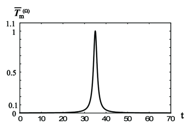
Figure 1: A graph of ${\cal{\bar{T}}}_{\text{m}}^{(\Omega)}$, which represents the angular frequency dependence of the magnon source term. Parameters we have used are, $2\tau\Omega\equiv t$, $\tau=2\times 10^{-6}[\text{s}]$, $\tilde{B}=1[\text{G}]$, $g=1$. Therefore $2\tau B/\hbar$ is $35$. This ${\cal{\bar{T}}}_{\text{m}}^{(\Omega)}$ has a sharp peak around $t=35$. This fact means that the magnon source term has a resonance structure with the applied transverse magnetic field.

2.4 Temperature dependence

Let us look into the temperature dependence of the magnon source term. To do this, we include the interaction of third-order in magnon operators. Then $V_{\Gamma}(t)$ is rewritten as

$$\begin{split}V_{\Gamma}(t)&=\Gamma(t)\int d^{3}xS^{x}(\mathbf{x})\\ &\simeq\Gamma(t)\int d^{3}x(\frac{S}{2})^{1/2}\bigg{\{}a(\mathbf{x}t)+a^{\dagger}(\mathbf{x}t)\\ &-\frac{1}{4S}\Big{[}a^{\dagger}(\mathbf{x}t)a^{\dagger}(\mathbf{x}t)a(\mathbf{x}t)+a^{\dagger}(\mathbf{x}t)a(\mathbf{x}t)a(\mathbf{x}t)\Big{]}\bigg{\}},\;\end{split}$$ (11)

and the magnon source term reads

$$\begin{split}\mathcal{T}_{\text{m}}(t)&=-\frac{(2S)^{1/2}}{\hbar}\ \text{Im}\bigg{<}\Gamma(t)\Big{[}a(\mathbf{x}t)+\frac{a^{\dagger}(\mathbf{x}t)a^{\dagger}(\mathbf{x}t)a(\mathbf{x}t)}{4S}\Big{]}\bigg{>}.\;\end{split}$$ (12)

Eq.(12) is calculated as

$$\begin{split}<\Gamma(t)a(t)>&=\int d^{3}x^{\prime}\int dt^{\prime}\Gamma(t)\Gamma(t^{\prime})\Big{[}(\frac{S}{2})^{1/2}G^{\text{r}}(t,t^{\prime})\\ &\ \ \ -\frac{i}{2(2S)^{1/2}}G^{\text{r}}(t,t^{\prime})G^{\text{<}}(t^{\prime},t^{\prime})\Big{]}+O(\Gamma^{3}),\;\end{split}$$ (13)

$$\begin{split}<\frac{\Gamma(t)}{4S}a^{\dagger}(t)a^{\dagger}(t)a(t)>&=\frac{i}{2(2S)^{1/2}}\int d^{3}x^{\prime}\int dt^{\prime}\\ &\cdot\Gamma(t)\Gamma(t^{\prime})G^{\text{a}}(t^{\prime},t)G^{\text{<}}(t,t)+O(\Gamma^{3}).\;\end{split}$$ (14)

Here $G^{\text{a}}$ and $G^{\text{<}}$ are the advanced and lesser Green’s functions, respectively. Because we focus on the behavior of the magnon source term at low temperature that we have neglected higher terms than the fourth-order in respect to magnon creation/annihilation operators. The Fourier transform of the lesser Green’s function satisfies, $\ G^{\text{<}}(\mathbf{k},\omega)=-f_{\text{B}}(\omega_{\mathbf{k}})[G^{\text{a}}(\mathbf{k},\omega)-G^{\text{r}}(\mathbf{k},\omega)]$, where $G^{\text{a}}(\mathbf{k},\omega)=[{\hbar\omega-\omega_{\mathbf{k}}-i\hbar/(2\tau)}]^{-1}$. Then $\cal{T}_{\text{m}}$ is calculated as

$$\begin{split}\cal{T}_{\text{m}}&=\frac{\Gamma^{2}_{0}}{4\hbar V}\bigg{[}S-\Big{(}1+\frac{1}{2^{3/2}}e^{-\beta B}\Big{)}e^{-\beta B}\Big{(}\frac{k_{\rm B}T}{4\pi D}\Big{)}^{3/2}\bigg{]}\\ &\ \ \ \ \ \ \ \ \cdot\bigg{[}\frac{\frac{\hbar}{2\tau}+(\hbar\Omega+B)\rm{sin}2\Omega t+\frac{\hbar}{2\tau}\rm{cos}2\Omega t}{(\hbar\Omega+B)^{2}+(\frac{\hbar}{2\tau})^{2}}\\ &\ \ \ \ \ \ \ \ \ \ +\frac{\frac{\hbar}{2\tau}+(\hbar\Omega-B)\rm{sin}2\Omega t+\frac{\hbar}{2\tau}\rm{cos}2\Omega t}{(\hbar\Omega-B)^{2}+(\frac{\hbar}{2\tau})^{2}}\bigg{]},\;\end{split}$$ (15)

where ${\beta}^{-1}$ is $k_{\text{B}}T$ ($k_{\text{B}}:$ Boltzmann constant). Here we have approximated the summation over the Bose distribution function as, $[(2\pi)^{3}/V]\sum_{\mathbf{k}}f_{\text{B}}(\omega_{\mathbf{k}})=2\pi\int_{-\infty}^{\infty}dkk^{2}[e^{\beta(Dk^{2}+B)}-1]^{-1}\simeq 2\pi\int_{-\infty}^{\infty}dk\ k^{2}e^{-\beta(Dk^{2}+B)}[1+e^{-\beta(Dk^{2}+B)}]$.

The time average of $\cal{T}_{\text{m}}$ becomes

$$\begin{split}\cal{\bar{T}}_{\text{m}}&=\frac{\Gamma^{2}_{0}}{4\hbar V}\bigg{[}S-\Big{(}1+\frac{1}{2^{3/2}}e^{-\beta B}\Big{)}e^{-\beta B}\Big{(}\frac{k_{\rm B}T}{4\pi D}\Big{)}^{3/2}\bigg{]}\\ &\ \ \ \cdot\bigg{[}\frac{\frac{\hbar}{2\tau}}{(\hbar\Omega+B)^{2}+(\frac{\hbar}{2\tau})^{2}}+\frac{\frac{\hbar}{2\tau}}{(\hbar\Omega-B)^{2}+(\frac{\hbar}{2\tau})^{2}}\bigg{]}\\ &=\frac{\Gamma^{2}_{0}}{4\hbar V}\frac{2\tau}{\hbar}{\cal{\bar{T}}}_{\text{m}}^{(\Omega)}{\cal{\bar{T}}}_{\text{m}}^{(T)},\\ \end{split}$$ (16)

where

$$\begin{split}{\cal{\bar{T}}}_{\text{m}}^{(T)}&\equiv S-\Big{(}1+\frac{1}{2^{3/2}}e^{-\beta B}\Big{)}e^{-\beta B}\Big{(}\frac{k_{\rm B}T}{4\pi D}\Big{)}^{3/2},\end{split}$$ (17)

is the temperature-dependent part and ${\cal{\bar{T}}}_{\text{m}}^{(\Omega)}$ is defined in eq.(10). When the temperature gets higher, the magnon source term decreases. This means that quantum and thermal fluctuations act in the opposite way, namely to increase and decrease the magnon source term, respectively. It is clear that eq.(16) reduces at the zero temperature to eq.(9).

3 Magnon Pumping

The spin pumping is an effect widely used to create a spin current by use of the magnetization precession. [4, 5, 6, 7, 8] Experiments have been carried out in junctions of metallic ferromagnets and nonmagnetic metals. According to the theory by Y.Tserkovnyak and A.Brataas,[9] the spin current pumped through the junction reads ${\mathbf{I}}_{\text{s}}^{\text{pump}}=[\hbar/(4\pi)][A_{\text{r}}\mathbf{m}\times(d{\mathbf{m}}/dt)-A_{\text{i}}(d{\mathbf{m}}/dt)]$, where $\mathbf{m}$ is the magnetization direction of a localized spin and $A_{\text{r}},A_{\text{i}}$ are the interface parameters. This result is understood by considering the spin continuity equation, $\nabla\cdot\mathbf{j}_{\text{s}}=-(\partial{\mathbf{m}}/\partial t)+{\mathbf{\cal{T}}}_{\text{s}}$, where $\mathbf{j}_{\text{s}}$ is the spin current density and ${\mathbf{\cal{T}}}_{\text{s}}$ is the spin relaxation torque. In fact, the spin continuity equation indicates that a spin current is generated when the magnetization is dynamic and/or when ${\mathbf{\cal{T}}}_{\text{s}}$ is finite. It has been well-known [17] that the main term of spin relaxation torque, ${\mathbf{\cal{T}}}_{\text{s}}$, has the form ${\mathbf{\cal{T}}}_{\text{s}}\propto\mathbf{m}\times(d\mathbf{m}/dt)$ in metals. As Brataas et al.[19] have pointed out, this torque ${\mathbf{\cal{T}}}_{\text{s}}$ is equivalent to the maximum spin current that can be drawn from the spin battery. The pumping formula for ${\mathbf{I}}_{\text{s}}^{\text{pump}}$ in metals is thus understood from the spin continuity equation. The relaxation torque plays an essential role in spin pumping in metals, and it is expected to be dominant also in the spin pumping in insulating ferromagnets. Our calculation of the relaxation torque term (i.e. the magnon source term) thus describes the spin pumping effect in insulators.

We have revealed that the magnon source term has a sharp peak around $\Omega=B/\hbar$, as a result of the resonance with a time-dependent transverse magnetic field when the angular frequency is appropriately adjusted as $\Omega=B/\hbar$. This fact is useful to enhance the magnon pumping effect because the external magnetic field, $B$, and the angular frequency of a transverse magnetic field, $\Omega$, is under our control.

Experimentally, the magnon pumping effect we have discussed can be identified by observing the temperature dependence of the pumped magnon current when $B$ is zero; $(\text{the pumped magnon current})\propto{\cal{\bar{T}}}_{\text{m}}^{(T)}\propto(\text{A}_{1}-\text{A}_{2}T^{3/2})$, where $\text{A}_{1}$ and $\text{A}_{2}$ are constants.

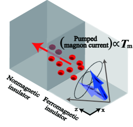
Figure 2: (Color online) A schematic picture of the magnon pumping by a time-dependent transverse magnetic field. Thick and short solid arrows represent localized spins, and thin and long ones external magnetic fields. Circles represent magnons. By way of resonance with a time-dependent transverse magnetic field, the magnon source term is enhanced, and an enhanced magnon current is pumped from the ferromagnetic insulator to the adjacent nonmagnetic insulator.

4 Summary

We have studied theoretically the magnon source term which represents the breaking of the magnon conservation law. We have revealed that the magnon source term has a resonance structure with an external time-dependent transverse magnetic field when the angular frequency of the applied magnetic field is tuned. This fact will be useful to enhance the magnon pumping effect in insulators. This magnon pumping effect is a new method for a generation of a magnon current (spin-wave spin current) without the gradient of an external magnetic field.

Appendix A Calculation of Equation.(7)

In this section, we briefly show the Langreth method, which is useful to evaluate the perturbation expansion of the Keldysh ( or contour-ordered) Green’s function. For simplicity here, we evaluate the magnon source term at zero temperature, eq.(7), as an example;

$$\begin{split}V_{\Gamma}(t)&\simeq\Gamma(t)\int d^{3}x(\frac{S}{2})^{1/2}\bigg{[}a(\mathbf{x}t)+a^{\dagger}(\mathbf{x}t)\bigg{]},\\ \mathcal{T}_{\text{m}}(t)&=-\frac{(2S)^{1/2}}{\hbar}\ \text{Im}\bigg{<}\Gamma(t)a(\mathbf{x}t)\bigg{>}.\\ \;\end{split}$$ (18)

We have only to estimate $<a(\mathbf{x}t)>$. It is evaluated as

$$\begin{split}<a(\tau)>&=\bigg{<}\text{T}_{\text{c}}\ a(\tau)\text{exp}\Big{[}-i\int_{\text{c}}d\tau^{\prime}V_{\Gamma}(\tau^{\prime})\Big{]}\bigg{>}\\ &\simeq-i(\frac{S}{2})^{1/2}\int d^{3}x^{\prime}\\ &\ \ \ \cdot\int_{\text{c}}d\tau^{\prime}\Gamma(\tau^{\prime})\Big{<}\text{T}_{\text{c}}\ a(\mathbf{x}\tau)a^{\dagger}(\mathbf{x^{\prime}}\tau^{\prime})\Big{>}\\ &\equiv-i(\frac{S}{2})^{1/2}\int d^{3}x^{\prime}{\cal{I}}.\;\end{split}$$ (19)

Here $\text{T}_{\text{c}}$ is the path-ordering operator defined on the Keldysh contour, c (see Fig.3). We express the Keldysh contour as a sum of the forward path, $c_{\rightarrow}$, and the backward path, $c_{\leftarrow}$; $c=c_{\rightarrow}+c_{\leftarrow}$. The integral on the Keldysh contour of eq.(19), ${\cal{I}}$, is executed by taking an identity into account

$$\begin{split}\int_{{\text{c}}}d\tau^{{\text{c}}}&=\int_{{\text{c}}_{\rightarrow}}d\tau^{{{\rightarrow}}}+\int_{{\text{c}}_{\leftarrow}}d\tau^{{{\leftarrow}}},\\ \;\end{split}$$ (20)

as

$$\begin{split}{\cal{I}}=i\int_{-\infty}^{\infty}d\tau^{\prime}\Gamma(\tau^{\prime})\Big{[}G^{\text{t}}(\tau,\tau^{\prime})-G^{\text{<}}(\tau,\tau^{\prime})\Big{]}.\;\end{split}$$ (21)

Here $G^{\text{t}}$ is the time-ordered Green’s function. By using the relation, $G^{\text{r}}(t,t^{\prime})=G^{\text{t}}(t,t^{\prime})-G^{\text{<}}(t,t^{\prime})$, we obtain eq.(7).

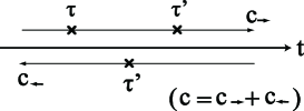
Figure 3: Keldysh contour, $c$. We have taken $\tau$ on forward path, ${\text{c}}_{\rightarrow}$. Even when $\tau$ is located on backward path, ${\text{c}}_{\leftarrow}$, the result of this calculation is invariant because each Green’s function, $G^{\text{r}}$, $G^{\text{a}}$, $G^{\text{<}}$, $G^{\text{>}}$ (the greater Green’s function ), is not independent; they obey, $G^{\text{r}}-$ $G^{\text{a}}$ $=G^{\text{>}}$ $-G^{\text{<}}$. Both the forward and backward paths are actually on the real axis but shifted slightly upwards and downwards, respectively, to distinguish them clearly.

References

- [1] S.Maekawa: Concepts in Spin Electronics (Oxford science publications, 2006).
- [2] I.Zutic, J.Fabian, and S.D.Sarma: Rev.Mod.Phys. (2004) 323.
- [3] Y.Tserkovnyak, A.Brataas, G.E.W.Bauer, and B.I.Halperin: Rev.Mod.Phys. (2005) 1375.
- [4] A.Takeuchi, K.Hosono, and G.Tatara: Phys.Rev.B. (2010) 144405.
- [5] S.Mizukami, Y.Ando, and T.Miyazaki: Phys.Rev.B. (2002) 104413.
- [6] R.H.Silsbee, A.Janossy, and P.Monod: Phys.Rev.B. (1979) 4382.
- [7] P. W. Brouwer: Phys.Rev.B. (1998) R10135.
- [8] P.Sharma and C.Chamon: Phys.Rev.Lett. (2001) 096401.
- [9] Y.Tserkovnyak and A.Brataas: Phys.Rev.Lett. (2002) 117601.
- [10] Y.K.Kato, R.C.Myers, A.C.Gossard, and D.D.Awschalom: Science. (2004) 1910.
- [11] Y.Kajiwara, K.Harii, S.Takahashi, J.Ohe, K.Uchida, M.Mizuguchi, H.Umezawa, H.Kawai, K.Ando, K.Takanashi, S.Maekawa, and E.Saitoh: Nature. (2010) 262.
- [12] F.Meier and D.Loss: Phys.Rev.Lett. (2003) 167204.
- [13] B.Wang, J.Wang, J.Wang, and D.Y.Xing: Phys.Rev.B. (2004) 174403.
- [14] T.Kita: Prog.Theor.Phys. (2010) 581.
- [15] J.Rammer and H.Smith: Rev.Mod.Phys. (1986) 323.
- [16] A.Kamenev: arXiv:0412296.
- [17] G.Tatara, H.Kohno, and J.Shibata: Physics Report. (2008).
- [18] H. Haug and A.P. Jauho: Quantum Kinetics in Transport and Optics of Semiconductors. (Springer New York, 2007) p.35.
- [19] A.Brataas, Y.Tserkovnyak, G.E.W.Bauer, and B.I.Halperin: Rhys.Rev.B. (2002) 060404(R).