Superconductivity in an extended Hubbard model with attractive interaction

Abstract

In this work, a two-dimensional one-band Hubbard model is investigated within a two-pole approximation. The model presents a non-local attractive potential $U(U<0)$ that allows the study of d-wave superconductivity and also includes hopping up to second-nearest-neighbors. The two-pole scheme has been proposed to improve the Hubbard-I approximation. The analytical results show a more complex form for the gap $\Delta(T)$, when compared to the one obtained in the latter approximation. Indeed, new anomalous correlation functions associated with the superconductivity are involved in the calculation of $\Delta(T)$. Numerical results in a range of temperatures are presented. Moreover, the structure of the quasiparticle bands and the topology of the Fermi surface are studied in detail in the normal state. Connections with some experimental results are also included.

I Introduction

Superconductivity in strongly correlated systems is a field with plenty of challenging problems. Several non-usual properties of high temperature superconductors (HTSC) cuprates still needed to be properly clarified. In particular, some experimental systems exhibit important deviations from the standard BCS theory. For instance, the superconductor gap behaviour as a function of temperature in some borocarbides display a non-monotonic feature at lower temperatures. In fact, such gap decreasing in $RNi_{2}B_{2}C(R=Dy,Ho,Er,Tm)$ and $ErNi_{2}B_{2}C$ borocarbides when the temperature decreases towards to $T=0$. This effect ascribed due to a competition between the superconductivity and antiferromagnetic correlations, which are absent in a weak coupling BCS-like superconductivity, appear naturally from the formulation which is shown in this work. Another quite interesting feature of HTSC systems is the behaviour found in some cuprates cuprates1 in the low doping region, the so called pseudo-gap region, which gives rise to an anomalous Fermi surface leading to a pseudo-gap.

In this very complex problem, a number of theories has been proposed in order to explain the presence of a pseudo-gap region cuprates . In the present formulation, we claim that the appearance of a pseudo-gap can be ascribed to a more detailed many-body treatment in which superconductor and AF correlations compete.

Although BCS-like approach BCS has been widely used to describe these physical systems, it is well recognized that superconductivity is a two-dimensional problem in which strong correlations play a fundamental role correlations . Thereby, we apply a two-pole approximation Roth69 ; Edwards95 ; Eleonir2005 to deal with the strong interaction coupling. Here we consider a d-wave symmetry gap and therefore, a non-local attractive interaction is used bib1 ; prbcaixeiro . The net attractive interaction $(U<0)$ may result, for example, from the elimination of the electron-phonon like coupling through a canonical transformation kittel or, alternatively, from an electronic mechanism proposed by Hirsch Hirsch2 which may produce, for a certain range of parameters, an effective attractive interaction.

In this work, we focused on the many-body renormalized normal state of these systems. Our obtained Fermi surface is consistent with recent claims in the literature cuprates1 ; singleton about the presence of hole-pockets due to antiferromagnetic correlations. Moreover, we discuss some thermodynamical properties of the superconducting regime, namely the critical temperature $T_{c}$, the zero temperature superconducting gap $\Delta_{0}$ and temperature dependence of the gap $\Delta(T)$ for various dopings $\delta\equiv 1-n_{T}$ (with $n_{T}=n_{\sigma}+n_{-\sigma}$) and interaction $U$. The $n_{\sigma}$ represents the average occupation per site of electrons with spin $\sigma=\uparrow,\downarrow$.

This paper is organized as follows. In the section II, we present a general formulation describing the model as well as the ingredients of the normal state, e.g. the quasi-particle and the special characteristics of the Fermi surface (FS). In section III, we present the superconducting state which appears from the application of the two-pole approximation. In section IV, we exhibit self-consistent numerical results and conclusions for both the normal and the superconducting states . The Appendix A briefly describes the main points involved in the two-pole approach whereas in the Appendix B the correlation functions involved in the Green’s functions governing the superconducting and the normal states are displayed.

II General Formulation

The Hamiltonian studied here is, in a standard notation

$$H=\sum_{\langle\langle ij\rangle\rangle\sigma}t_{ij}d_{i\sigma}^{{\dagger}}d_{j\sigma}+U\sum_{\langle ij\rangle\sigma}n_{i,\sigma}^{d}n_{j,-\sigma}^{d}-\mu\sum_{i\sigma}d_{i\sigma}^{{\dagger}}d_{i\sigma}$$ (1)

where $\langle\langle...\rangle\rangle$ indicates the sum over the first and the second-nearest-neighbors of $i$ and $\mu$ is the chemical potential. The two-dimensional dispersion relation is given by:

$$\varepsilon_{\vec{k}}=2t(\cos(k_{x}a)+\cos(k_{y}a))+4t_{2}\cos(k_{x}a)\cos(k_{y}a).$$ (2)

In the present work, we adopted the two-pole approximation Roth69 ; Edwards95 which consists in choosing a set of operators describing the most important excitations of the system. The details of the method are given in Appendix A. In the present case, the set of operators considered is $\left\{d_{i,\sigma},n_{i,-\sigma}^{d}d_{i,\sigma},d_{i,-\sigma}^{\dagger},n_{i,\sigma}^{d}d_{i-\sigma}^{\dagger}\right\}$. The first two are associated with the normal state whereas the last two are associated with the superconductivity Edwards95 ; Eleonir2005 . Following the method exhibited in the Appendix A, the one-particle Green’s function for the normal state is:

$$G_{N\sigma}^{dd}(\vec{k},\omega)=\frac{Z_{1\vec{k}\sigma}}{\omega-\omega_{1\vec{k}\sigma}}+\frac{Z_{2\vec{k}\sigma}}{\omega-\omega_{2\vec{k}\sigma}}$$ (3)

with

$$Z_{1\vec{k}\sigma}=\frac{1}{2}+\frac{\overline{U}-2U_{1}-\varepsilon_{\vec{k}}+W_{\vec{k}\sigma}}{2X_{\vec{k}\sigma}},$$ (4)

$$Z_{2\vec{k}\sigma}=1-Z_{1\vec{k}\sigma}$$ (5)

and

$$\overline{U}=\frac{U_{2}+n_{-\sigma}(U_{1}-2U_{2})}{n_{-\sigma}(1-n_{-\sigma})}.$$ (6)

The quasiparticle bands are:

$$\omega_{1\vec{k}\sigma}=\frac{\overline{U}+\varepsilon_{\vec{k}}-2\mu+W_{\vec{k}\sigma}}{2}-\frac{X_{\vec{k}\sigma}}{2},$$ (7)

$$\omega_{2\vec{k}\sigma}=\omega_{1\vec{k}\sigma}+X_{\vec{k}\sigma}$$ (8)

where

$$X_{\vec{k}\sigma}=\sqrt{(\overline{U}-\varepsilon_{\vec{k}}+W_{\vec{k}\sigma})^{2}+4U_{1}(\varepsilon_{\vec{k}}-W_{\vec{k}\sigma})+\widetilde{U}}$$ (9)

and

$$\widetilde{U}=\frac{4U_{2}(U_{2}-U_{1})}{n_{-\sigma}(1-n_{-\sigma})}.$$ (10)

The effective interactions $U_{1}$, $U_{2}$ and the band shift $W_{\vec{k}\sigma}$ are defined in the Appendix A (see Eqs. (38)-(40)). Here, as we are assuming a paramagnetic state of a translationally invariant system, $\langle n_{i,\sigma}\rangle=\langle n_{i,-\sigma}\rangle=\langle n_{-\sigma}\rangle$. It should be noticed that, due to many body effects, in the pole structure of the Green’s functions, in the normal paramagnetic phase, there is a spin-spin correlation function which exhibit only antiferromagnetic (AF) short range correlations. That is not in contradiction in our previous paramagnetic assumption. Moreover, in order to simplify the notation, we write $\langle n_{-\sigma}\rangle=n_{-\sigma}$.

From the Green’s function in equation (3), we find the spectral function

$$A_{\sigma}(\vec{k},\omega)=-\frac{1}{\pi}\mbox{Im}[{G_{N\sigma}^{dd}(\vec{k},\omega)}].$$ (11)

The Fermi surface is obtained from $A_{\sigma}(\vec{k},\omega=0)$.

III The superconducting state

In the superconducting state, the Green’s function $G^{dd}$ is written as:

$$G_{S\sigma}^{dd}(\vec{k},\omega)=\frac{A^{\prime}(\omega)-(\omega+E_{11})(1+n_{-\sigma}^{2}\frac{U}{\theta})^{2}\Delta_{\vec{k}}^{2}}{P(\omega)}$$ (12)

where

$$A^{\prime}(\omega)=\alpha_{0}+\alpha_{1}\omega+\alpha_{2}\omega^{2}+\alpha_{3}\omega^{3}$$ (13)

with

$$\alpha_{0}= (E_{12}^{2}-E_{11}E_{22})(E_{22}-2n_{-\sigma}E_{12}+n_{-\sigma}^{2}E_{11})$$ (14)

$$\alpha_{1}= 2n_{-\sigma}\widetilde{n}E_{11}E_{12}-(\widetilde{n}+2n_{-\sigma})n_{-\sigma}E_{12}^{2}-n_{-\sigma}^{3}E_{11}^{2}$$ (15)

$$-E_{22}[E_{22}+2n_{-\sigma}(n_{-\sigma}E_{11}-2E_{12})]$$

$$\alpha_{2}= n_{-\sigma}^{2}(1-n_{-\sigma})^{2}E_{11}$$ (16)

$$\alpha_{3}= n_{-\sigma}^{2}(1-n_{-\sigma})^{2}$$ (17)

and $\widetilde{n}=(1+n_{-\sigma})$. The $E_{nm}$ are elements of the energy matrix (32) and the quantity $P(\omega)$, is defined as:

$$P(\omega) =[(\omega-E_{11})(n_{-\sigma}\omega-E_{22})-(n_{-\sigma}\omega-E_{12})^{2}]$$ (18)

$$\times[(\omega+E_{11})(n_{-\sigma}\omega+E_{22})-(n_{-\sigma}\omega+E_{12})^{2}]~{}~{}~{}$$

$$+\Delta_{\vec{k}}^{2}(A_{1}-A_{2}\omega)$$

with

$$A_{1}=a_{0}+a_{1}\frac{U}{\theta}+\left[a_{2}+\Delta_{\vec{k}}^{2}(1+n_{-\sigma}^{2}\frac{U}{\theta})^{2}\right]\left(\frac{U}{\theta}\right)^{2}$$ (19)

and

$$A_{2}=(1+n_{-\sigma}^{2}\frac{U}{\theta})^{2}+n_{-\sigma}^{2}(1-n_{-\sigma})^{2}\left(\frac{U}{\theta}\right)^{2}.$$ (20)

The quantities $a_{0}$, $a_{1}$, $a_{2}$ and $\theta$, are given by:

$$a_{0} =E_{11}^{2}$$ (21)

$$a_{1} =2E_{12}(2n_{-\sigma}E_{11}-E_{12})$$ (22)

$$a_{2} =E_{22}^{2}-4n_{-\sigma}E_{12}E_{22}+2n_{-\sigma}^{2}(E_{12}^{2}+E_{11}E_{22})$$ (23)

and

$$\theta=tn_{01\sigma}-U(D_{01\sigma}+2\langle S_{1}^{z}S_{0}^{z}\rangle)$$ (24)

with the correlation functions $n_{01\sigma}$, $D_{01\sigma}$ and $\langle S_{1}^{z}S_{0}^{z}\rangle$ defined in the Appendix B.

The main reason that we are adopting the d-wave symmetry is that we are following reference Edwards95 where it is claimed that for a large number of HTSC material d-wave gap symmetry is the most relevant.

Moreover, the d-wave symmetry follows also from the fact that in our Hamiltonian we consider an attractive delocalized interaction term. Actually the extended s-wave symmetry is more favoured for an attractive local interaction as discussed in bib1 .

For the particular case of pairing with $d$-wave symmetry, the gap function is

$$\Delta_{\vec{k}}=2\Delta[cos(k_{x})-cos(k_{y})],$$ (25)

where $\Delta$ is the gap function amplitude. Following the procedure described in references Edwards95 ; Eleonir2005 , the self-consistent gap function has been obtained from the Green’s function:

$$G_{\sigma}^{dd^{\dagger}}(\vec{k},\omega)=-\frac{\Delta_{\vec{k}}(\beta_{0}+\beta_{1}\omega^{2})}{P(\omega)}$$ (26)

in which,

$$\Delta=-2\theta\Delta\frac{1}{L}\sum_{\vec{q}}[cos(q_{x})-cos(q_{y})]^{2}F_{1\vec{q}\sigma}$$ (27)

and

$$F_{1\vec{q}\sigma}=\frac{1}{2\pi i}\oint f(\omega)[\frac{\beta_{0}+\beta_{1}\omega^{2}}{P(\omega)}]d\omega.$$ (28)

The $\beta_{0}$ and $\beta_{1}$ are

$$\beta_{0} = n_{-\sigma}^{2}(1-n_{-\sigma})^{2}\frac{U}{\theta}$$ (29)

$$\beta_{1} = E_{1}^{2}-[E_{2}^{2}-2E_{1}E_{2}+\Delta_{\vec{q}}^{2}(1+n_{-\sigma}^{2}\frac{U}{\theta})^{2}]\frac{U}{\theta}~{}~{}~{}~{}~{}~{}$$ (30)

with $E_{1}=E_{12}-n_{-\sigma}E_{11}$ and $E_{2}=E_{22}-n_{-\sigma}E_{12}$.

IV Self-consistent results and conclusions

Firstly, we discuss the numerical results for the normal state ($T>T_{c}$).

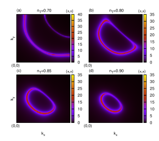
Figure 1: (Color)The spectral function $A(\vec{k},\omega=0)$ representing the Fermi surface for different dopings $\delta=1-n_{T}$. The model parameters considered here are $U=8t$, $t=-1.0$ eV, $t_{2}=0.3|t|$ and $k_{B}T=0.1|t|$ ($k_{B}$ is the Boltzmann constant).

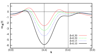
Figure 2: (Color) The quasiparticle bands intercepted by the chemical potential ($\mu=0$). The model parameters and the temperature are the same as in figure 1.

Figure 1 shows the FS for four different doping values $\delta$. In (a), $\delta=0.30$, a well defined electron-like FS is found. However, in (b) when $\delta$ is decreased to $\delta=0.20$, the topology of the FS changes, with the emergence of a hole-pocket enclosing the nodal point $(\frac{\pi}{2},\frac{\pi}{2})$. As a consequence, due to low spectral intensity, a pseudogap appears near the antinodal points $(\pi,0)$ and $(0,\pi)$. Further decrease in $\delta$ intensifies the presence of the pseudo-gap as shown in (c)-(d). This unusual behaviour is due to the strong antiferromagnetic correlations coming from the band shift $W_{\vec{k}\sigma}^{d}$ Edwards95 ; Eleonir2010 defined in equation (40).

The effects described above, are corroborated by the quasiparticle band calculation exhibited in figure 2 which displays the quasiparticle band for distinct doping values $\delta$. In fact, while in the higher doping regime the quasiparticle bands cross the Fermi level near $(\frac{\pi}{2},\frac{\pi}{2})$ and near the antinodal point $(0,\pi)$, in the lower doping regime the quasiparticle band crosses the Fermi level only near the nodal point $(\frac{\pi}{2},\frac{\pi}{2})$. Such a behavior gives rise to a pocket around $(\frac{\pi}{2},\frac{\pi}{2})$. On the other hand, as the quasiparticle band does not touch the Fermi level near $(0,\pi)$, a pseudogap emerges in that region. As far as we know, the emergence of the pseudogap due to an attractive $U$ in a strong correlation regime, is for the first time presented here. The kink observed near the $(\pi,\pi)$ point of the quasiparticle band is caused by the strong antiferromagnetic correlations associated with $\langle\vec{S_{j}}\cdot\vec{S_{i}}\rangle$, which are maximum in Q$=(\pi,\pi)$. The Q is the antiferromagnetic wave-vector.

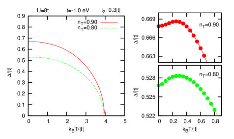
Figure 3: (Color)The main figure shows the gap function amplitude versus the temperature for $U=8t$, $t=-1.0$ eV, $t_{2}=0.3|t|$ and two different occupations $n_{T}$. The small figures show the regions of low temperatures where the gap presents an unusual behavior.

Now we discuss some thermodynamical properties associated to the superconducting state. In figure 3 we describe the gap function amplitude $\Delta(T)$ for $U=8t$ and two different occupations $n_{T}$, in the lower doping regime. One sees that for a given $U$ (in a characteristic strong coupling regime $|\frac{U}{t}|>>1$), the zero temperature gap for $n_{T}=0.90$ is higher than the corresponding one for $n_{T}=0.80$. Furthermore, the temperature where a non-superconducting phase arises is higher for $n_{T}=0.90$, i.e., $T_{c}(n_{T}=0.90)>T_{c}(n_{T}=0.80)$. It should be noted that in both cases for $n_{T}$, in the region of low $T$, there is a increase in the value of the gap amplitude as compared to the zero gap amplitude value. This unusual behavior is due to the effect of the strong correlations, since that in the BCS weak correlated regime, $\Delta(0)$ is always greater than $\Delta(T)$.

We stress that in our case this non-monotonic behavior at low temperatures is mainly due to correlation functions in the pole structure of the superconduction Green’s function (see equations (12) and (26)). To be more precise, we have found in our self-consistent calculation a complex interplay between the SC gap behaviour and the AF type short range correlations.

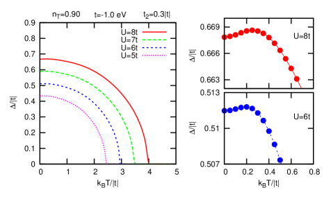
Figure 4: (Color)The main figure shows the gap function amplitude versus the temperature for $n_{T}=0.90$ and different values of $U$. The remaining parameters are identical to figure 3. The small figures show the regions of low temperatures for two values of $U$. For low temperatures, the gap presents an unusual behavior.

Figure 4 displays the value of the gap amplitude $\Delta(T)$ as a function of temperature for several values of $U$, in the strong correlation regime ($|\frac{U}{t}|>>1$). In all cases, for $n_{T}=0.90$, we note that when $U$ increases, $T_{c}$ increases also, and the same unusual behavior for $\Delta(T)$ appears for very low $T$. We have calculated the gap function amplitude for several values of $U$, for different $n_{T}$ ($n_{T}=0.80$ and 0.70), and the same behavior is observed.

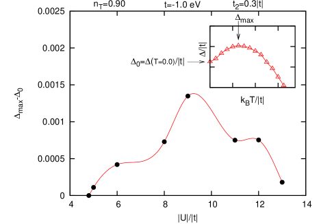
Figure 5: (Color)The difference between $\Delta_{max}$ and $\Delta_{0}$ as a function of $|\frac{U}{t}|$. The inset shows as $\Delta_{max}$ and $\Delta_{0}$ have been obtained.

A very interesting result is shown in figure 5. Here, we plot $\Delta_{max}$ - $\Delta_{0}$ for several values of $|\frac{U}{t}|$. One noted that when $U$ increases, $\Delta_{max}$ - $\Delta_{0}$ increases also, until a special value (in our calculation $|\frac{U}{t}|\simeq 8$) where $\Delta_{max}$ - $\Delta_{0}$ is a maximum and then, $\Delta_{max}$ - $\Delta_{0}$ tends toward zero in a very high value of $U$. When such behavior appears, one has attained the $|U|\rightarrow\infty$ limit. Moreover, it should be noted that this unusual behavior occurs for a critical low value of $|U|$, (in our calculation $|\frac{U}{t}|\simeq 4$), which is a signature of the onset of a characteristic $|\frac{U}{t}|>>1$, signaling the appearance of a strong correlation regime.

Our results are in qualitatively agreement concerning the Fermi surface in underdoping region with other approaches using the t-J model tJ . The reason of such agreement is that in both approaches the spin spin correlation functions renormalize the band structure giving rise to the appearance of hole-pockets.

Finally, in order to complement our present calculations, we need to discuss the higher doping regime $n_{T}\lesssim 0.80$. Moreover, a detailed discussion of the effect of external pressure, which affects mainly the ratio $\frac{t_{2}}{t}$ angi , is needed. These further calculations, are now in progress.

Appendix A Two-pole approximation

In the present two-pole approximation Roth69 ; Edwards95 , the Green’s functions are defined as:

$${\bf G}\left(\omega\right)={\bf N}(\omega{\bf N}-{\bf E})^{-1}{\bf N}$$ (31)

where, E and N are the energy and the normalization matrices given by

$$E_{nm}=\left\langle\left[\left[A_{n},H\right]_{-},A_{m}^{{\dagger}}\right]_{\left(+\right)}\right\rangle$$ (32)

and

$$N_{nm}=\langle[A_{n},A_{m}^{{\dagger}}]_{\left(+\right)}\rangle.$$ (33)

In equations (32)-(33), $[...,...]_{(+)-}$ denote the (anti)commutator, and $\langle...\rangle$, the thermal average. The set of operators $\{A_{n}\}$ must satisfy, within some approximation, the relation $\left[A_{n},H\right]_{-}=\sum_{m}K_{nm}A_{m}$.

For the normal state of the model (1), the energy matrix is given by,

$${\bf E}=\left[\begin{tabular}[]{cc}$\varepsilon_{\vec{k}}-\mu+U_{1}~{}~{}~{}~{}~{}~{}$&$\varepsilon_{\vec{k}}-\mu+U_{2}$\\ \\ $\varepsilon_{\vec{k}}-\mu+U_{2}~{}~{}~{}~{}~{}~{}$&$\varepsilon_{\vec{k}}n_{\sigma}^{2}-\mu+U_{2}+\overline{n}W_{\vec{k}\sigma}$\end{tabular}\right]$$ (37)

with

$$U_{1}=2U\sum_{l}\langle n_{l,-\sigma}\rangle,$$ (38)

$$U_{2}=2U\sum_{l}\langle n_{l,-\sigma}n_{i,-\sigma}\rangle$$ (39)

and $\overline{n}=n_{-\sigma}(1-n_{-\sigma})$. The correlation function $D_{il-\sigma}=\langle n_{i-\sigma}n_{l-\sigma}\rangle$ is defined in equation (43). The band shift $W_{\vec{k}\sigma}$, can be written as:

$$\overline{n}W_{\vec{k}\sigma}^{d}=-\sum_{\langle\langle j\neq 0\rangle\rangle}t_{0j}(n_{0j\sigma}-2m_{0j\sigma})+\sum_{\langle\langle j\neq 0\rangle\rangle}t_{0j}e^{i\vec{k}\cdot\vec{R}_{j}}h_{j\sigma}$$ (40)

with $n_{ij\sigma}$, $m_{ij\sigma}$ and $h_{j\sigma}$ defined below.

Appendix B Correlation functions

The correlation function $n_{ij\sigma}=\langle d_{i\sigma}^{\dagger}d_{j\sigma}\rangle$, is given by:

$$n_{ij\sigma}=\frac{1}{2\pi iL}\sum_{\vec{k}}\oint e^{i\vec{k}\cdot(\vec{R}_{j}-\vec{R}_{i})}f(\omega)G_{S\sigma}^{dd}(\vec{k},\omega)d\omega$$ (41)

with $G_{S\sigma}^{dd}$ defined in equation (12). Assuming $i=0$ and $t_{0j}=t$ for the $z$ nearest-neighbors, only one value of $n_{0j\sigma}$, namely $n_{01\sigma}$, is necessary. Considering the same for the second-nearest-neighbors $t_{2}$, we have:

$$n_{01\sigma}=\frac{1}{2\pi iL}\sum_{\vec{k}}\oint\frac{\epsilon_{\vec{k}}}{(t+t_{2})z}f(\omega)d\omega.$$ (42)

By using the original Roth’s scheme Roth69 , the correlation function $D_{ij\sigma}=\langle n_{i\sigma}n_{j\sigma}\rangle$, is calculated and written as:

$$D_{ij\sigma}=n_{\sigma}^{2}-\frac{\alpha_{ij\sigma}n_{ij\sigma}+\beta_{ij\sigma}m_{ij\sigma}}{1-\beta_{ii,\sigma}\beta_{ii,-\sigma}}$$ (43)

with $m_{ij\sigma}=\langle d_{i\sigma}^{\dagger}n_{j-\sigma}d_{j\sigma}\rangle$ given by

$$m_{ij\sigma}=\frac{1}{2\pi iL}\sum_{\vec{k}}\oint e^{i\vec{k}\cdot(\vec{R}_{j}-\vec{R}_{i})}f(\omega)G_{S\sigma}^{n_{2}d}(\vec{k},\omega)d\omega$$ (44)

and

$$\alpha_{ij\sigma}=\frac{n_{ij\sigma}-m_{ij\sigma}}{1-n_{-\sigma}}$$ (45)

$$\beta_{ij\sigma}=\frac{m_{ij\sigma}/n_{-\sigma}-n_{ij\sigma}}{1-n_{-\sigma}}.$$ (46)

The $D_{01\sigma}$ can be obtained assuming again $i=0$ and $t_{0j}=t$ for the $z$ nearest-neighbors, as it has been done in $n_{01\sigma}$.

The Green’s function $G_{S\sigma}^{n_{2}d}$ in 44, is:

$$G_{S\sigma}^{n_{2}d}(\vec{k},\omega)=\frac{n_{-\sigma}\left[A^{\prime\prime}(\omega)-A^{\prime\prime\prime}(\omega)(1+n_{-\sigma}^{2}\frac{U}{\theta})\Delta_{\vec{k}}^{2}\right]}{P(\omega)}$$ (47)

where

$$A^{\prime\prime}(\omega)=\gamma_{0}+\gamma_{1}\omega+\gamma_{2}\omega^{2}+\gamma_{3}\omega^{3}$$ (48)

with

$$\gamma_{0}= (E_{12}^{2}-E_{11}E_{22})[E_{3}+n_{-\sigma}(E_{12}-E_{11})]$$ (49)

$$\gamma_{1}= n_{-\sigma}E_{11}[E_{12}(1+3n_{-\sigma})-n_{-\sigma}(E_{11}+\widetilde{n}E_{22})]$$ (50)

$$+E_{22}E_{3}+n_{-\sigma}E_{12}(3E_{3}-n_{-\sigma}E_{12})$$

$$\gamma_{2}= n_{-\sigma}(1-n_{-\sigma})^{2}E_{12}$$ (51)

$$\gamma_{3}= n_{-\sigma}^{2}(1-n_{-\sigma})^{2}.$$ (52)

The quantities $E_{3}$ and $\widetilde{n}$ are:

$$E_{3}=E_{22}-E_{12}~{}~{}~{}~{}\mbox{and}~{}~{}~{}~{}\widetilde{n}=1+n_{-\sigma}.$$ (53)

The term $A^{\prime\prime\prime}$ introduced in equation (47) is defined as:

$$A^{\prime\prime\prime}(\omega)=\omega(1+n_{-\sigma}^{2}\frac{U}{\theta})+E_{11}+\frac{U}{\theta}[n_{-\sigma}(E_{12}+E_{11})-E_{12}].$$ (54)

The denominator of the Green’s function $G^{n_{2}d}$, is given in equation (18).

The term $h_{j\sigma}$ presented in the band shift (40), is given by:

$$h_{j\sigma}=B_{j\sigma}+\langle\vec{S_{j}}\cdot\vec{S_{0}}\rangle$$ (55)

with

$$B_{j\sigma} = -\langle S_{j}^{z}S_{0}^{z}\rangle-\frac{\alpha_{j\sigma}n_{0j\sigma}^{d}+\beta_{j\sigma}m_{j\sigma}}{1-\beta_{\sigma}\beta_{-\sigma}}$$ (56)

$$-\frac{\alpha_{j\sigma}n_{0j-\sigma}^{d}+\beta_{j\sigma}(n_{0j-\sigma}^{d}-m_{j-\sigma})}{1-\beta_{\sigma}}$$

and

$$\langle\vec{S_{j}}\cdot\vec{S_{0}}\rangle=\frac{1}{2}\left(\langle S_{j}^{+}S_{0}^{-}\rangle+\langle S_{j}^{-}S_{0}^{+}\rangle\right)+\langle S_{j}^{z}S_{0}^{z}\rangle.$$ (57)

Particularly, in the paramagnetic state, $\langle S_{j}^{+}S_{0}^{-}\rangle=\langle S_{j}^{-}S_{0}^{+}\rangle$, then, $\langle\vec{S_{j}}\cdot\vec{S_{0}}\rangle$ can be written as:

$$\langle\vec{S_{j}}\cdot\vec{S_{0}}\rangle=\langle S_{j}^{+}S_{0}^{-}\rangle+\langle S_{j}^{z}S_{0}^{z}\rangle$$ (58)

where,

$$\langle S_{j}^{+}S_{0}^{-}\rangle=\langle d_{j\sigma}^{\dagger}d_{j-\sigma}d_{0-\sigma}^{\dagger}d_{0\sigma}\rangle=-\frac{\alpha_{j\sigma}n_{0j,-\sigma}^{d}+\beta_{j,\sigma}m_{j,-\sigma}}{1+\beta_{\sigma}}$$ (59)

and

$$\langle S_{j}^{z}S_{0}^{z}\rangle = \frac{(1-\beta_{-\sigma})}{2}\left[(n_{\sigma}^{d})^{2}-\frac{\alpha_{j\sigma}n_{0j\sigma}+\beta_{j\sigma}m_{j\sigma})}{1-\beta_{\sigma}\beta_{-\sigma}}\right]-\frac{\alpha_{-\sigma}n_{\sigma}^{d}}{2}.$$ (60)

The correlation functions $n$, $m$, $\alpha$ and $\beta$, are defined in equations (41), (44), (45) and (46), respectively.

In order to calculate $n_{ij\sigma}$ and $m_{ij\sigma}$ in the normal state, it is necessary to consider $\Delta=0$ in the Green’s functions $G_{S\sigma}^{dd}$ and $G_{S\sigma}^{n_{2}d}$ defined in equations (12) and (47). In this case, $G_{S\sigma}^{dd}\rightarrow G_{N\sigma}^{dd}$ and $G_{S\sigma}^{n_{2}d}\rightarrow G_{N\sigma}^{n_{2}d}$.

References

(1)
Patrick A. Lee, Naoto Nagaosa, and Xiao-Gang Wen,
Rev. Mod. Phys. 78, 17 (2006).
(2)
T. Baba at al, Phys. Rev. Lett. 100, 017003 (2008),
Yu. G. Naidyuk at al, J. Phys.: Conference Series, 150, 052178 (2009).
(3)
A. Kanigel, M. R. Norman, H. Ding, M. Randeria et al., Nature Physics 2, 447 (2006).
(4)
G. M. Japiassu, M. A. Continentino and A. Troper, Phys. Rev. B45, 2986 (1992).
(5)
E. Dagotto, Rev. Mod. Phys. 66, 763 (1994)
(6)
L. M. Roth, Phys. Rev. 184, 451 (1969).
(7)
J. Beenen and D. M. Edwards, Phys. Rev. B52, 13636 (1995).
(8)
E. J. Calegari, S. G. Magalhaes and A. A. Gomes, Eur. Phys. J. B45, 485 (2005).
(9)
E. S. Caixeiro and A. Troper, J. Appl. Phys. 105, 07E307 (2009).
(10)
E. S. Caixeiro and A. Troper, Phys. Rev. B 82, 014502 (2010).
(11)
C. Kittel, Quantum Theory of Solids, John Wiley & Sons, Inc., New York (1963), p. 150.
(12)
J.E. Hirsch In: Theories of High Temperature Superconductivity, edited by J. Woods Halley, Addison-Wesley, Reading MA (1988), p. 241.
(13)
N. Harrison, R. D. McDonald and J. Singleton, Phys. Rev. Lett. 99 206406 (2007).
(14)
E. J. Calegari, S. G. Magalhaes, Int. J. of Mod. Phys. B (in press).
(15) G. G. N. Angilella, R. Pucci and Fabio Siringo, Phys. Rev. B 54, 15471 (1996).
(16) E. S. Caixeiro and A. Troper, Physica B 404, 3102 (2009).
(17)
M. M. Korshunov and S. G. Ovchinnikov, Eur. Phys. J. B57, 271 (2007),
Shiro Sakai, Yukitoshi Motome and Masatoshi Imada, Phys. Rev. Lett. 102 056404 (2009),
Shiro Sakai, Yukitoshi Motome and Masatoshi Imada, Phys. Rev. B82 134505 (2010).