Evidence for a bicritical point in the XXZ Heisenberg antiferromagnet on a simple cubic lattice

Abstract

The classical Heisenberg antiferromagnet with uniaxial exchange anisotropy, the XXZ model, in a magnetic field on a simple cubic lattice is studied with the help of extensive Monte Carlo simulations. Analyzing, especially, various staggered susceptibilities and Binder cumulants, we present clear evidence for the meeting point of the antiferromagnetic, spin–flop, and paramagnetic phases being a bicritical point with Heisenberg symmetry. Results are compared to previous predictions based on various theoretical approaches.

Uniaxially anisotropic Heisenberg antiferromagnets in a magnetic field have been studied quite extensively in the past, both experimentally and theoretically rev1 ; rev2 . Usually, they display, at low temperatures and fields, the antiferromagnetic phase and, when increasing the field, the spin–flop phase. A prototypical model describing these phases as well as, possibly, multicritical points, is the Heisenberg model with a uniaxial exchange anisotropy, the XXZ model

$${\cal H}=J\sum\limits_{i,j}\left[\,\Delta(S_{i}^{x}S_{j}^{x}+S_{i}^{y}S_{j}^{y})+S_{i}^{z}S_{j}^{z}\,\right]\;-\;H\sum\limits_{i}S_{i}^{z}$$ (1)

where $J(>0)$ is the exchange coupling between classical spins, $(S_{i(j)}^{x},S_{i(j)}^{y},S_{i(j)}^{z})$, of length one at neighboring sites, $i$ and $j$, on a simple cubic lattice, $\Delta$ is the uniaxial exchange anisotropy, $1>\Delta>0$, and $H$ is the applied magnetic field along the easy axis, the $z$–axis. The phase diagram of the model has been investigated already several years ago, using, among others, mean–field theory Gorter , Monte Carlo (MC) simulations LanBin , and high temperature series expansions Mourit . The transition between the antiferromagnetic (AF) and spin–flop (SF) phases seems to be of first order, while the boundaries of the paramagnetic (P) phase to the AF and SF phases are believed to be continuous transitions in the Ising and XY universality classes, respectively. Moreover, based on renormalization group analyses in one–loop–order, a bicritical point in the Heisenberg universality class had been proposed, at which the three different phases meet FN ; KNF . This scenario has been questioned on the basis of renormalization group calculations in high–loop–order CPV , where the bicritical point has been argued to be unstable against a tetracritical point Aha , which, in turn, may be unstable towards transitions of first order in the vicinity of the meeting point of the three phases. However, a subsequent renormalization group analysis in two–loop–order Folk suggests that a bicritical point in the Heisenberg universality class can not be excluded.

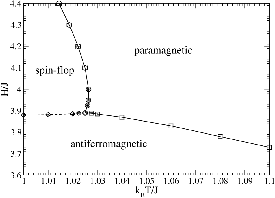
Figure 1: Phase diagram of the XXZ model on a cubic lattice with exchange anisotropy $\Delta=0.8$ in the vicinity of the AF–SF–P point, as obtained from the present MC simulations.

As has been noted quite recently HWS , not only AF and SF phases, but also biconical (BC) structures KNF may play an important role in the XXZ model. Indeed, such BC structures are degenerate ground states at the critical field separating AF and SF configurations at zero temperature. For the XXZ model on a square lattice, these degenerate BC fluctuations lead to a narrow disordered phase intervening between the AF and SF phases at low temperatures, giving, presumably, rise to a ’hidden tetracritical point’ HWS ; Zhou at zero temperature. A recent Monte Carlo study bann for the XXZ antiferromagnet on a simple cubic lattice showed that biconical structures, arising from the degenerate ground states, also occur at low temperatures close to the transition between the AF and SF phases. But they do not destroy the direct transition of first order between these two phases, in accordance with the behavior predicted by mean–field and other, more reliable theories.

In that recent MC study bann of the three–dimensional XXZ model, Eq. (1), at fixed anisotropy, $\Delta=0.8$, continuous phase boundaries of Ising type, for the AF–P transition, and of XY type, SF–P, as well as the transition line of first order, AF–SF, have been identified. The position of the meeting (or AF–SF–P) point has been estimated, $k_{B}T/J=1.025\pm 0.015$ and $H/J=3.9\pm 0.03$, without determining critical properties of the AF–SF–P point. The aim of the present paper is to deal with this intriguing aspect, using extensive MC simulations.

Here, the standard Metropolis algorithm LanBinMC with single spin–flips is applied. Employing full periodic boundary conditions, lattices with $L^{3}$ sites, are considered. $L$ ranges from 4 to 40, with the main focus on the sizes $L$= 8, 16, 24, and 32, to study systematically finite–size effects. MC runs with, at least, $10^{7}$ MC steps per site for the larger lattices, are performed. Error bars are estimated by averaging over, at least, three independent realizations. In this way, data of the desired accuracy are obtained, and there is no need to use other, perhaps, more powerful MC algorithms.

To map the phase diagram, we study, especially, quantities related to the Ising, XY, and Heisenberg order parameters. In particular, we monitor, apart from the absolute values of the staggered longitudinal, $m^{z}_{st}$, transverse, $m^{xy}_{st}$, and isotropic, $m^{xyz}_{st}$, magnetizations, the corresponding staggered susceptibilities, $\chi^{z}_{st},\chi^{xy}_{st}$, and $\chi^{xyz}_{st}$, as well as the corresponding Binder cumulants Binder , $U^{z},U^{xy}$, and $U^{xyz}$. To our knowledge, the isotropic quantities, being crucial to identify a bicritical point with Heisenberg symmetry, had not been included in previous MC simulations.

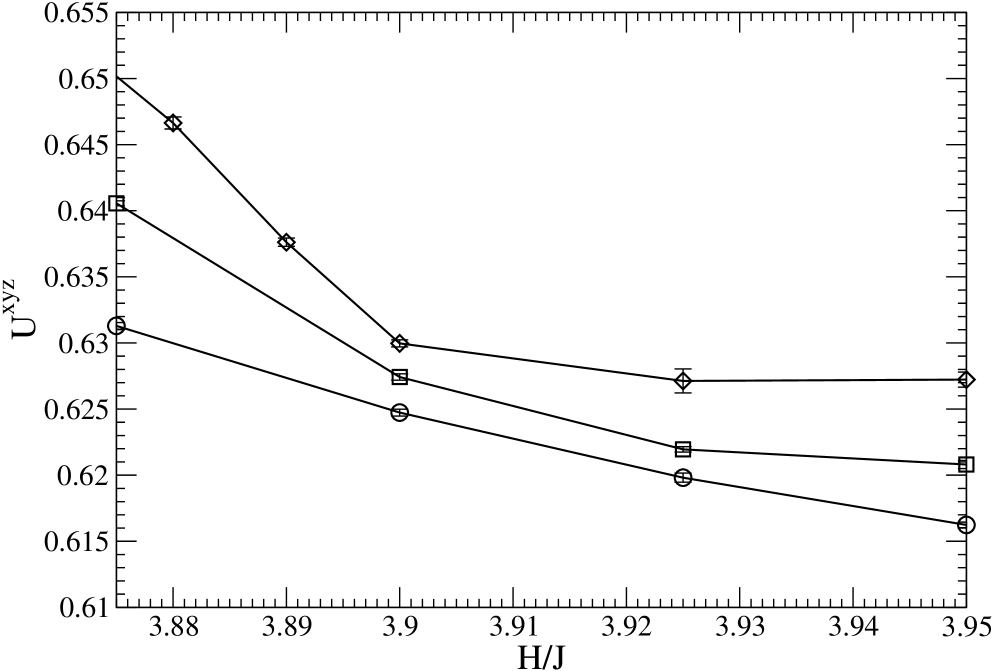
Figure 2: Isotropic Binder cumulant $U^{xyz}$, at $k_{B}T/J=1.0225$, varying the field, for lattice sizes $L=16$ (circles), 24 (squares), and 32 (diamonds).

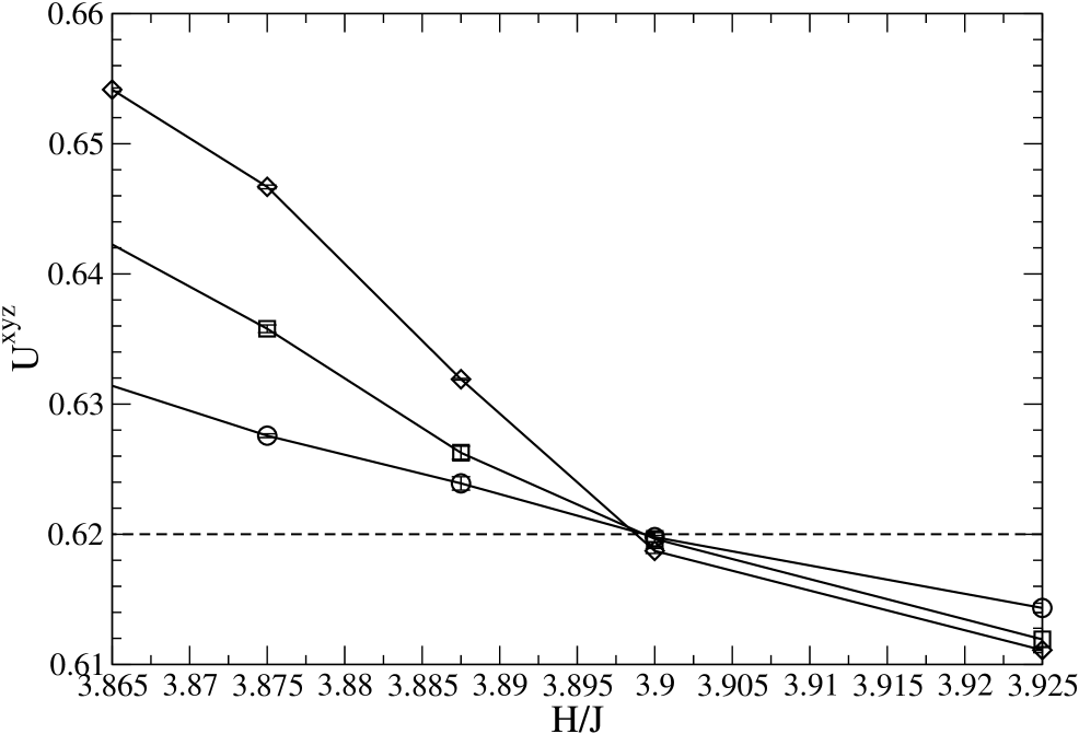
Figure 3: As for Fig. 2, at $k_{B}T/J=1.025$, including $(U^{xyz})^{*}$ as dashed line hase2 ; pec .

The phase diagram, in the ($k_{B}T/J,H/J$)–plane, in the vicinity of the AF–SF–P point is depicted in Fig.1. As before, we set $\Delta$= 0.8. The shown estimates for the transition lines are based on usual finite–size analyses Barber . In particular, to determine the AF–P boundary, with the transition being in the Ising universality class, the size dependence of the height and position of the maximum in the longitudinal staggered susceptibility, $\chi^{z}_{st}$, allows for reliable estimates. $U^{xy}$ turns out to be very useful in estimating the SF–P transition line. There one observes rather small finite–size correction terms to the critical Binder cumulant for cubic lattices in the XY universality class hase1 , $(U^{xy})^{*}$= 0.586.., with the critical Binder cumulant being the cumulant at the transition in the thermodynamic limit, $L\rightarrow\infty$. Finally, the AF–SF phase boundary of first order is readily identified from the location of the maxima in $\chi^{z}_{st}$ and $\chi^{xy}_{st}$.

The resulting phase diagram confirms and refines previous, independent MC findings bann . Note that the present results allow to locate the AF–SF–P point accurately, $k_{B}T/J=1.025\pm 0.0025$ and $H/J=3.89\pm 0.01$, reducing appreciably the error bars obtained in the previous MC study, as mentioned above.

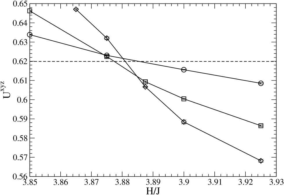
Figure 4: As for Fig. 3, at $k_{B}T/J=1.03$.

Most importantly, critical properties of the AF–SF–P point are studied. In case of a bicritical point with Heisenberg symmetry, the critical Binder cumulant $(U^{xyz})^{*}$ is expected hase2 ; pec to acquire the value 0.620 ($\pm 0.003$), using periodic boundary conditions for lattices of cubic shape. Note that, in general, the critical Binder cumulant, in a given universality class, may depend on boundary condition, system shape, and lattice anisotropy of the interactions Binder ; CD ; SeSh .

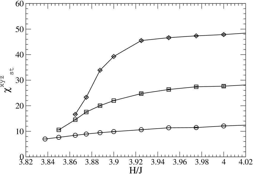
Figure 5: Staggered isotropic susceptibility $\chi^{xyz}_{st}$ at $k_{B}T/J=1.025$ for $L$= 16 (circles), 24 (squares), and 32 (diamonds).

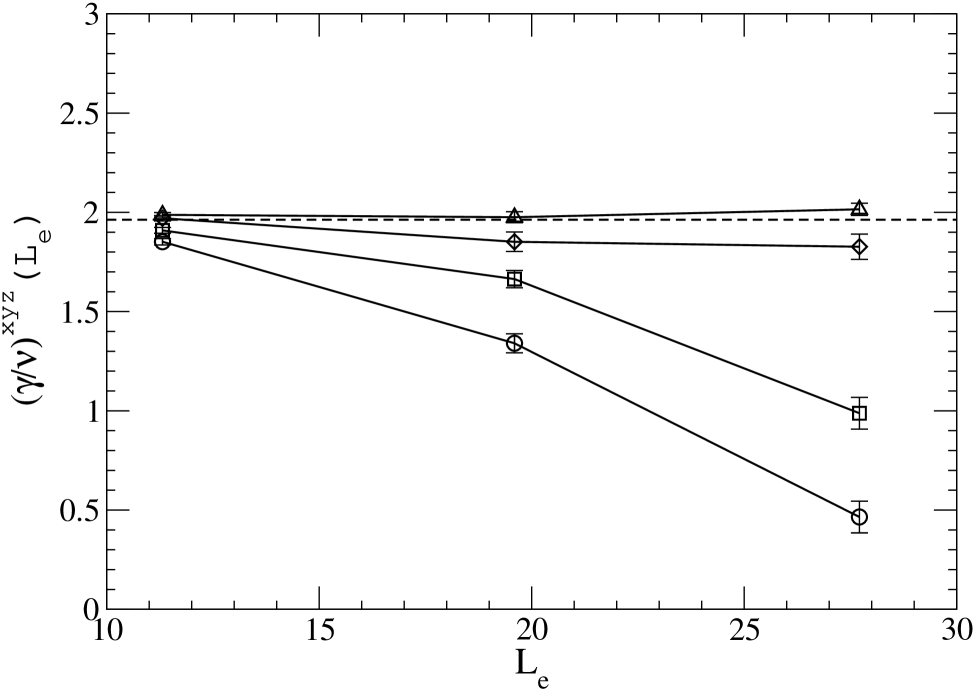
Figure 6: Effective critical exponent $(\gamma/\nu)^{xyz}(L_{e})$ of the staggered isotropic susceptibility, see Eq. (2), at $k_{B}T/J=1.025$ and $H/J$= 3.865 (circles), 3.875 (squares), 3.8875 (diamonds), and 3.90 (triangles). The dashed line marks the asymptotic critical exponent in the Heisenberg universality class PV .

In Figs. 2, 3, and 4 the size dependent isotropic Binder cumulant $U^{xyz}$ is displayed near the AF–SF–P point, at three fixed temperatures, $k_{B}T/J$= 1.0225, 1.025, and 1.03, varying the field to cross the boundary of the AF phase, see also Fig. 1. We may distinguish three different scenarios. At the lowest temperature, $k_{B}T/J=1.0225$, see Fig. 2, the cumulant increases with larger system sizes at all fields, so that there are no intersection points for cumulants of different sizes. This behavior is in accordance with being at a temperature below that of the AF–SF–P point. Indeed, $U^{xyz}$ tends to 2/3 in the AF and SF phases in the thermodynamic limit, and there is no indication of a transition of Heisenberg symmetry. At $k_{B}T/J=1.025$, see Fig. 3, all intersection points of the cumulants, for lattices of sizes $L$= 16, 24, and 32, occur closely to the critical Heisenberg value, $(U^{xyz})^{*}\approx 0.620$. This fact may be interpreted as evidence for being in the immediate vicinity of a bicritical point of Heisenberg symmetry. Actually, moving to higher temperatures, another scenario shows up. There are still intersection points of the cumulants for different lattice sizes, but they shift for larger lattices to lower and lower values below that of the critical cumulant in the Heisenberg universality class. This trend is already seen for $k_{B}T/J=1.0275$, and it is quite pronounced at $k_{B}T/J=1.03$, as depicted in Fig. 4. In any event, the observations on the isotropic Binder cumulant are completely consistent with the existence of a bicritical point with Heisenberg symmetry at $k_{B}T/J=1.025\pm 0.0025$.

This suggestion is supported by the behavior of the isotropic staggered susceptibility $\chi^{xyz}_{st}$. Simulation data at fixed $k_{B}T/J=1.025$ are shown in Fig. 5. At first sight, there seems to be no hint for criticality of Heisenberg type, because $\chi^{xyz}_{st}$ as a function of field exhibits no maximum. However, additional information is provided by the standard discrete effective critical exponent, at given temperature and field,

$$(\gamma/\nu)^{xyz}(L_{e})=\ln(\chi^{xyz}_{st}(L_{1})/\chi^{xyz}_{st}(L_{2}))/\ln(L_{1}/L_{2})$$ (2)

for successive sizes $L_{1}>L_{2}$ and with the effective length $L_{e}=\sqrt{L_{1}L_{2}}$. In case of critical behavior in the Heisenberg universality class, the effective exponent would approach, for $L_{e}\longrightarrow\infty$, the known PV asymptotic value $(\gamma/\nu)^{xyz}$= 1.96… In fact, as shown in Fig. 6, the effective exponent seems to approach closely that value at $H/J=3.8875\pm 0.0125$. Obviously, at those fields one is in a (crossover) critical region governed by the Heisenberg fixed point, in accordance with the findings for the isotropic Binder cumulant. The suggestion is corroborated by the behavior of the staggered longitudinal and transverse susceptibilities. Both quantities show pronounced maxima, when varying the field at $k_{B}T/J$= 1.025. The size dependence of the peak position allows us to estimate the critical field. Within the error bars, both susceptibilities lead to the same critical field, $H/J=3.895\pm 0.005$, indicating, again, the closeness of the bicritical point.

It should be mentioned that we did, in addition, a preliminary MC study at a rather strong anisotropy, $\Delta=0.2$. The AF–SF–P point is estimated to be at about $k_{B}T/J=0.2095\pm 0.0005$ and $H/J=5.825\pm 0.0025$. In the immediate vicinity of that point, the isotropic Binder cumulant shows similar features to the ones discussed above. We tend to believe that the AF–SF–P point in the XXZ Heisenberg antiferromagnet on a simple cubic lattice is generically a bicritical point with Heisenberg symmetry.

I should like to thank R. Folk, G. Bannasch, T.–C. Dinh, and D. Peters for very useful discussions.

References

- (1) Y. Shapira, in Multicritical Phenomena , ed. by R. Pynn and A. Skjeltorp (Plenum Press, New York and London, 1984), p.35; and references therein.
- (2) W. Selke, M. Holtschneider, R. Leidl, S. Wessel, G. Bannasch, and D. Peters, Physics Procedia 6, 84 (2010); and references therein.
- (3) C. J. Gorter and T. Van Peski-Tinbergen, Physica 22, 273 (1956).
- (4) D. P. Landau and K. Binder, Phys. Rev. B 17, 2328 (1978).
- (5) O. G. Mouritsen, E. K. Hansen, and S. J. K. Jensen, Phys. Rev. B 22, 3256 (1980).
- (6) M. E. Fisher and D. R. Nelson, Phys. Rev. Lett. 32, 1350 (1974).
- (7) J. M. Kosterlitz, D. R. Nelson, and M. E. Fisher, Phys. Rev. B 13, 412 (1976).
- (8) P. Calabrese, A. Pelissetto, and E. Vicari, Phys. Rev. B 67, 054505 (2003).
- (9) A. Aharony, J. Stat. Phys. 110, 659 (2003).
- (10) R. Folk, Yu. Holovatch, and G. Moser, Phys. Rev. E 78, 041124 (2008).
- (11) M. Holtschneider, S. Wessel, and W. Selke, Phys. Rev. B 75, 224417 (2007).
- (12) C. G. Zhou, D. P. Landau, and T. C. Schulthess, Phys. Rev. B 76, 024433 (2007).
- (13) G. Bannasch and W. Selke, Eur. Phys. J. B 69, 439 (2009).
- (14) D. P. Landau and K. Binder, A Guide to Monte Carlo Simulations in Statistical Physics (University Press, Cambridge, 2005).
- (15) K. Binder, Z. Physik B- Cond. Matt. 43, 119 (1981).
- (16) M. N. Barber, in Phase Transitions and Critical Phenomena , ed. by C. Domb and J. L. Lebowitz (Academic Press, New York, 1983), Vol. 8.
- (17) M. Hasenbusch and T. Török, J. Phys. A- Math. Gen. 32, 6361 (1999).
- (18) P. Peczak, A. M. Ferrenberg, and D. P. Landau, Phys. Rev. B 43, 6087 (1991).
- (19) M. Hasenbusch, J. Phys. A- Math. Gen. 34, 8221 (2001).
- (20) X. S. Chen and V. Dohm, Phys. Rev. E 70, 056136 (2004).
- (21) W. Selke and L. N. Shchur, J. Phys. A- Math. Gen. 38, L739 (2005).
- (22) A. Pelissetto and E. Vicari, Phys. Rep. 368, 549 (2002).