Disruption Management with Rescheduling of Trips and Vehicle Circulations

Abstract

This paper introduces a combined approach for the recovery of a timetable by rescheduling trips and vehicle circulations for a rail-based transportation system subject to disruptions. We propose a novel event-based integer programming (IP) model. Features include shifting and canceling of trips as well as modifying the vehicle schedules by changing or truncating the circulations. The objective maximizes the number of recovered trips, possibly with delay, while guaranteeing a conflict-free new timetable for the estimated time window of the disruption. We demonstrate the usefulness of our approach through experiments for real-life test instances of relevant size, arising from the subway system of Vienna. We focus on scenarios in which one direction of one track is blocked, and trains have to be scheduled through this bottleneck. Solving these instances is made possible by contracting parts of the underlying event-activity graph; this allows a significant size reduction of the IP. Usually, the solutions found within one minute are of good quality and can be used as good estimates of recovery plans in an online context.

1 Introduction

1.1 Disruption Management in Passenger Traffic

Mobility of people is of growing importance in modern societies. For instance, especially in densely populated European cities, public transportation systems form a relevant economic factor. However, possible disruption of operations in such systems will always remain unavoidable. Increased pressure towards economical operation has amplified the impact and the frequency of such disruptions. Being often optimized to the limit, transportation systems have become more interconnected, and therefore more vulnerable to disruptions.

This makes it indispensable to develop more advanced methods for disruption management of passenger traffic. Railway disruption management is defined in Jespersen-Groth et al. [1] as the process of finding a new timetable by rerouting, delaying, or canceling trains and rescheduling the resources like rolling stock and the crew such that the new timetable is feasible with respect to the new schedules. This has to be performed while the effects of disruptions are still unfolding, that is, disruption management is an online problem.

The recovery of the timetable, the vehicle schedule, and the crew schedule is usually performed sequentially. While previous work has focused on either delay management (i.e., making sure that the delay of passengers and the inconvenience caused by missed trains is kept low) or on deriving new circulations on a given dispatching timetable, a particular aspect that has yet to be considered from a scientific side is to combine rescheduling of trips and vehicle circulations to obtain a feasible dispatching timetable. The goal is to perform as many trips of the original timetable as possible. Clearly, this is an important next step when further advancing optimization towards real-time methods for stabilizing rail-based transportation systems.

1.2 Related Work

The challenges and problems connected with passenger railway transportation have been intensively studied for the last decades, and operations research methods have been successfully applied. For example, Liebchen investigated the optimization of periodic timetables [2]. However, in daily operation, unforeseen events occur and may lead to disruptions of the timetable. Different aspects of this problem have been considered, and various approaches and models exist. A general framework for the problems and solution methods in disruption management can be found in [1]. The problem we investigate in this paper is closely related to the delay management problem. Mixed-integer approaches for it are introduced by Schöbel [3, 4] and extended by capacity constraints for the tracks [5]. Schachtebeck [6] adds circulation constraints to the model and performs a matching at the depots to prevent a large delay from spreading into the next circulation activity. The computational complexity of the original delay management problem is investigated in [7]: it turns out to be NP-hard, even in special cases, see also [8]. Simulation studies can be found in [9, 10, 11]. Törnquist [12] gives an overview over the existing models and decision support systems. He also investigates the disturbance management on $n$-tracks [13]. Gatto and Widmayer consider related problems as an online job shop model [14]. A decision support system for rolling stock rescheduling during disruption, where the rolling stock is balanced according to a given dispatching timetable, is provided by Nielsen [15].

In this paper, we focus on scenarios in which one direction of a track network has to be shutdown, such that trains have to be scheduled through a bottleneck. This leads to the track allocation problem studied by Borndörfer and Schlechte [16], which is shown to be NP-hard in [8]. A column generation approach to timetabling trains though a corridor is presented by Cacchiani et al. [17]. Huisman et al. developed column generation approaches to reschedule rail crew [18] and solved the combined crew rescheduling problem with retiming of trips by allowing small changes to the train timetables [19]. An overview of models and methods for similar problems that arise in the airline context can be found in Clausen [20].

None of the above papers considers rescheduling of trips and circulations as an integral part of deriving a feasible dispatching timetable. Clearly, we can imagine real-life scenarios that require an integrated approach for disruption management, e.g., in an online situation with trains already circulating in the rail network and an infeasible timetable due to heavy disruptions.

1.3 Our Contribution

In this paper, we introduce a combined approach for rescheduling trips and vehicle circulations in order to deal with unplanned disruptions. We derive a new re-optimized dispatching timetable with respect to a feasible new vehicle schedule that performs as much of the original trips as possible. Especially in subway systems, the utilization of the system is high. The high frequency of trains circulating in the system, the limited possibilities for overtaking, swapping tracks, and temporarily parking, as well as the bottleneck sections caused by disruptions force us to add stronger resource restrictions and integrate further possibilities into the model in order to obtain a feasible dispatching timetable. Our main mathematical contributions are an appropriate model based on integer programming that combines rescheduling of trips and circulations, as well as a mathematical contraction technique for simplifying the model. On the practical side, we are able to demonstrate the usefulness of this mathematical optimization approach by providing optimal and near-optimal solutions for a system of real-life instances that are based on the subway system of Vienna.

The rest of this paper is organized as follows. In the following section, we describe detailed aspects of disruptions in the operation of rail-based transportation. This leads to an optimization model based on integer linear programming. Mathematical aspects of solving real-life instances are discussed, and computational results are presented before we conclude with a discussion of future work.

2 Disruption in Public Transport

Disturbances in the daily operation of public passenger transport cannot be avoided. This can include delays caused by longer waiting times, because an unexpected number of passengers enter or leave the train, a driver arriving late at a relief point, or a technical problem with the mechanism of an automatic door. These disruptions lead to small delays, which usually can be absorbed by the buffer times integrated into the timetable. If bigger disruptions occur, e.g., a vehicle breaks down or a part of the track requires unplanned work, this causes a temporary shutdown on a track section. Such disruptions lead to severe violations of the timetable, which have to be resolved by the dispatchers.

As an illustrating example, consider a blocked track section on a $2$-track network. A possible option includes rerouting trips, which originally use the blocked track, via the opposite track. This leads to a large number of conflicts on that track section, because trains driving into opposite directions have to share the same track resources and compete for free time slots to pass trough this bottleneck. Consider two trains that are scheduled to enter the shared track section in opposite directions at the same time. Assume that the minimum transit time is 5 minutes and the minimum safety time between two trains using the same track in opposite direction is one minute. If the cycle time is 5 minutes and we allow a maximum delay of 5 minutes, it is not possible to schedule both trains through the bottleneck.

Depending on the length of the bottleneck and the frequency of the railway system, updating the timetable by delaying trips will not suffice. If trains queue up in front of the bottleneck, passenger travel time will increase dramatically. More precisely, the dispatcher has different possibilities for dealing with this situation. The timetabling perspective includes that

1. trips can be delayed within a certain time window and

2. trips can be canceled.

In addition rescheduling of the vehicle circulations allows that

1. trains can be instructed to truncate their circulation and turn early, in order to serve trips initially planned for a different train,

2. trains can be used to shuttle inside the single-track sections,

3. trains can return early to a depot, and

4. replacement vehicles can be used.

Usually, timetabling and vehicle scheduling are planned sequentially. Recently, research has focused more and more on integrating different steps of the planning process, as proposed in [21]. If heavy disruptions occur, these two aspects are strongly interweaved and need to be handled at the same time.

In the following, we present a model based on integer linear programming that finds a feasible disposition timetable and new vehicle schedules. It respects the capacity constraints of the tracks and allows dropping trips and early turns. The goal is to return to the initial timetable within a certain time horizon.

3 Our Model

3.1 A Graph Representation

In the following we consider a rail network $G=(\mathcal{S},\mathcal{J})$ with $\mathcal{S}$ and $\mathcal{J}$ representing the set of stations and tracks and a given dispatching timetable $\pi$ that includes the schedule for each vehicle in $\mathcal{V}$. Our model for disruption management with rescheduling of trips and vehicle circulations is based on the widely used concept of an event-activity network. This structure was suggested by Serafini and Ukovich [22] and also used by Nachtigall [23] for periodic timetabling problems, see also [24]. In the context of delay management problems event-activity networks are used in [4]. We use a model similar to [6] and extend the event-activity network to account for early turnarounds and capacity constraints at the station platforms.

An event-activity $\mathcal{N}=(\mathcal{E},\mathcal{A})$ is a directed graph, where the nodes in $\mathcal{E}$ denote the events and the edges in $\mathcal{A}$ are called activities. In our setting the timetable $\pi$ consists of scheduled trips. A trip connects two stations with a specified train via a certain track. A sequence of consecutive trips between two terminal stations is called a line. A sequence of lines is called a circulation. Each trip generates two events: a departure event $v\in\mathcal{E}_{\text{dep}}$ from a station, and an arrival event $w\in\mathcal{E}_{\text{arr}}$ at an adjacent station. These two events are connected by a driving activity $a=(v,w)$. Together, they model a constraint between those events, meaning that event $w$ cannot happen before event $v$ has taken place, plus the minimum duration $L_{a}$ assigned to activity $a$.

Similar to [4], we distinguish between different types of activities.

Train activities $(\mathcal{A}_{\text{train}})$ represent the driving, waiting and turning operations of a train.

1. Driving activities ($\mathcal{A}_{\text{drive}}\subset\mathcal{E}_{\text{dep}}\times\mathcal{E}_{\text{arr}}$) represent scheduled trips between two stations.

2. Waiting activities ($\mathcal{A}_{\text{wait}}\subset\mathcal{E}_{\text{arr}}\times\mathcal{E}_{\text{dep}}$) represent the scheduled waiting times at a station to let passengers enter and leave the train.

3. Turning activities ($\mathcal{A}_{\text{turn}}\subset\mathcal{E}_{\text{arr}}\times\mathcal{E}_{\text{dep}}$) connect an arrival event with a departure event, but in addition to waiting arcs, the events connected by a turning activity do not belong to trips on the same line; instead, they represent the possibility for trains to truncate their current circulation and continue on an different line.

Headway activities can be split into two subsets of activities that deal with the limited capacity of tracks between two stations $(\mathcal{A}_{\text{track}})$ or on a platform ($\mathcal{A}_{\text{station}})$:

1. The headway activities ($\mathcal{A}_{\text{track}}\subset\mathcal{E}_{\text{dep}}\times\mathcal{E}_{\text{dep}}$) model the headway condition between two events that share the same track resource between two stations. For each $a=(v,w)\in\mathcal{A}_{\text{track}}$, there is a corresponding activity $\tilde{a}=(w,v)\in\mathcal{A}_{\text{track}}$ so that together they model a precedence constraint, i.e., indicate which of the departure events will take place first. Thus, only one of each pair of activities can be active.

2. If we have to route trains through a corridor consisting of several stations on a single track, we have to introduce a second kind of headway activity ($\mathcal{A}_{\text{station}}\subset\mathcal{E}_{\text{arr}}\times\mathcal{E}_{\text{arr}}$). These have to make sure that trains driving in opposite directions do not enter the same platform and block each other; in other words, they ensure that the departure event of some train takes place before another train arrives at the same platform. Unfortunately, two arrival events could imply more than one pair of precedence constraints. In fact, this kind of headway activities involves four events, i.e. each possible departure event corresponding to the arrival events. In our model we add the possibilities for trains to turn at certain points, so the point of time a train may enter a station is strongly connected to the direction of the successive trip of the train.

   In addition, the headway constraints transmits the priority decision taken from the precedence constraints on the tracks of one side of the station to the other side.

   As an example, consider two trains $k,l\in\mathcal{V}$ and three station $A,B,C\in\mathcal{S}$. Train $k$ moves from station $A$ through station $B$ to station $C$ and train $l$ drives into the opposite directions from station $C$ through station $B$ to station $A$. So if the departure event from station $A$ to $B$ of train $k$ is scheduled to take place before the departure event of train $l$ at station $B$ to $A$, then also train $k$ has to depart from station $B$ to $C$ before train $l$ leaves station $C$ in opposite directions to station $B$.

In our model trains could be ordered to return to a depot and reserve trains may be inserted. Therefore, we extend the event-activity network by adding depots $D_{i}\in\mathcal{D}$ and replacement capacities $R^{D_{i}}$ for each depot. For each trip that ends at a station connected to a depot we add a trip to the depot, i.e., a departure event at the station and an arrival event at the depot connected by a driving activity. The sets $\mathcal{E}_{\text{depot}}$ contains the arrival events at the depots and $\mathcal{A}_{\text{return}}$ the corresponding driving activities. Trains stored in the depots may become reinserted after a minimum idle time, so analogously, the arrival events at a depot become connected to the departure events of possible follow on trips. Similarly, replacement capacities are inserted, by adding an event $r\in\mathcal{E}_{\text{repl}}$ for each depot supplying replacement vehicles and connecting them to the network.

Despite rescheduling the timetable events our model should be able to modify the vehicle schedules to find feasible new circulations, perform unplanned turns or to return to a depot at certain station. Therefore,a classical flow model is integrated. Each activity $a\in\mathcal{A}_{\text{train}}$ can transport a flow of at most one unit. For each event $i\in\mathcal{E}$, the outflow equals the inflow. Thus, every event with an ingoing activity arc that transports one unit of flow has a predecessor event and due to flow conservation is also connected to a successor event. The goal is to find feasible flows in the network, i.e., trains always have a sequence of following trips and do not stand idle and block the tracks.

A feasible timetable $\pi\in\mathbb{N}_{0}^{\mathcal{E}}$ assigns a time $\pi_{v}$ to each timetable event $v\in\mathcal{E}$ and a feasible flow through the network represents the circulation of trains.

3.2 Integer Programming Formulation

A solution of the following integer programming model yields a new feasible dispatching timetable $\pi^{\ast}\in\mathbb{Z}_{+}^{\mathcal{E}}$ and vehicle schedule in case of a disruption based on the original timetable $\pi\in\mathbb{Z}_{+}^{\mathcal{E}}$ and the corresponding vehicle circulations.

$$\max\sum_{v\in\mathcal{E}_{\text{dep}}}\sum_{a\in\delta^{+}(v)}c_{a}\,y_{a}$$ (1)

subject to

$$M(1-y_{a})+x_{w}+\pi_{w} \geq x_{v}+\pi_{v}+L^{min}_{a} \forall a=(v,w)\in\mathcal{A}_{\text{train}},$$ (2)

$$M(1-y_{a})+x_{w}+\pi_{w} \leq x_{v}+\pi_{v}+L^{max}_{a} \forall a=(v,w)\in\mathcal{A}_{\text{drive}},$$ (3)

$$M(3-\sum_{a\in\delta^{+}(w)}y_{a}- \sum_{a\in\delta^{+}(v)}y_{a}-g_{vw})$$

$$+x_{w}+\pi_{w} \geq x_{v}+\pi_{v}+L_{vw} \forall(v,w)\in\mathcal{A}_{\text{track}},$$ (4)

$$g_{vw}+g_{wv} =1 \forall(v,w)\in\mathcal{A}_{\text{track}},$$ (5)

$$-M(3-y_{vw}-y_{{v^{\prime}w^{\prime}}}- h_{vv^{\prime}})$$

$$+x_{w}+\pi_{w}+S_{vv^{\prime}} \leq x_{v^{\prime}}+\pi_{v^{\prime}} \forall(v,w),(v^{\prime},w^{\prime})\in\mathcal{A}_{\text{train}}:$$

$$(v,v^{\prime})\in\mathcal{A}_{\text{station}},$$ (6)

$$h_{vv^{\prime}}+h_{{v^{\prime}v}} =1 \forall(v,v^{\prime})\in\mathcal{A}_{\text{station}},$$ (7)

$$\sum_{a\in\delta^{-}(v)}y_{a}-\sum_{a\in\delta^{+}(v)}y_{a} =0 \forall v\in\mathcal{E}_{\text{dep}}\cup\mathcal{E}_{\text{arr}},$$ (8)

$$\sum_{a\in\delta^{-}(v)}y_{a}-\sum_{a\in\delta^{+}(v)}y_{a} \leq 1 \forall v\in\mathcal{E}_{\text{depot}},$$ (9)

$$\sum_{a\in\delta^{+}(v)}y_{a} \leq R^{D_{i}} \forall v\in\mathcal{E}_{\text{repl}},D_{i}\in\mathcal{D},$$ (10)

$$y_{a} \in\{0,1\} \forall a\in\mathcal{A},$$ (11)

$$x_{v} \in\mathbb{Z}_{+} \forall v\in\mathcal{E},$$ (12)

$$g_{a} \in\{0,1\} \forall a\in\mathcal{A}_{\text{track}},$$ (13)

$$h_{a} \in\{0,1\} \forall a\in\mathcal{A}_{\text{station}}$$ (14)

The variables of the model are as follows: $y$ is the circulation of trains, $x_{v}$ determines the delay of event $v$, $g_{a}$ and $h_{a}$ represent precedence constraints (see below). In the following, we successively discuss the constraints of the above model.

The objective function (1) aims at maximizing the number of trips that still will be served in the re-optimized dispatching timetable $\pi^{\ast}$, possibly with delay. Because the frequency of most subway systems is quite high, canceling few trips will lead to only a minor delay and inconvenience for the passengers. Therefore, minimizing the overall delay, as it is done in most publications about delay management, is only a secondary goal.

A trip is served if the corresponding departure event $v\in\mathcal{E}_{\text{dep}}$ has an outflow of one unit of flow, i.e., $a=(v,w)\in\mathcal{A}_{\text{drive}}$ is part of a train circulation. We can attach an additional cost coefficient $c_{a}$ to each driving activity $a$; this allows a weighting of the trips.

Given an original timetable $\pi$ and a corresponding vector $x\in\mathbb{Z}_{+}^{\mathcal{E}}$, representing the delays $x_{v}$ of each event $v$, Constraints (2) require that if an activity $a=(v,w)$ is in the solution, the earliest time for event $w$ to start is the starting time of the predecessor event $\pi_{v}$, plus the occurred delay $x_{v}$ and the minimum duration $L^{min}_{a}$ of activity $a$. With respect to the buffer times, a delay $x_{v}$ of event $v$ might cause a delay $x_{w}$ of the successor event $w$. We assume that the driving times are symmetric. Constraints (3) make sure that a driving activity $a$ is bounded by a maximal duration $L^{max}_{a}$, which includes possible buffer times and safety margins, but should not be too large to prevent trains being idle for a long period of time. The precedence constraints formulated by (4) and (5) for shared track resources, come in pairs for $(v,w),(w,v)\in\mathcal{A}_{\text{track}}$ and ensure that conflicting events $v,w\in\mathcal{E}_{\text{dep}}$ that use the same track resource are correctly scheduled to prevent deadlocks and keep safety margins. The model implies

$$g_{vw}=\left\{\begin{array}[]{r@{\quad: \quad}l}1&\text{if event }v\text{ takes place before }w,\\ 0&\text{otherwise,}\end{array}\right.$$

where $L_{vw}$ represents the minimal waiting time for event $w$ to start if $w$ is scheduled after $v$. If the trips corresponding to the departure events $v,w\in\mathcal{E}_{\text{dep}}$ use the track in the same direction, $L_{vw}$ is the safety margin between both departure events; if the track is used in opposite direction, $L_{vw}$ contains the maximum allowed transit time for the trip and a safety margin $S_{vw}$.

Similarly the precedence constraints (6), (7) for the tracks inside a station ensure that no two trains use the same platform at the same time, where the model implies

$$h_{vv^{\prime}}=\left\{\begin{array}[]{r@{\quad: \quad}l}1&\text{if event }w\text{ takes place before event, }v^{\prime}\\ 0&\text{otherwise.}\end{array}\right.$$

Regarding two conflicting arrival events $v,v^{\prime}\in\mathcal{E}_{\text{arr}}$ at some station and their corresponding departure events $w,w^{\prime}\in\mathcal{E}_{\text{dep}}$ with $a=(v,w)$, $\tilde{a}=(v^{\prime},w^{\prime})\in\mathcal{A}_{\text{train}}$ denoting the activities, if the solution contains both activities ($y_{a}=y_{\tilde{a}}=1$) and $h_{vv^{\prime}}=1$, departure event $w$ takes place before the arrival event $v^{\prime}$ at the platform with respect to the safety margin $S_{vv^{\prime}}$ (see Figure 1).

The safety margins $S_{vw}$ and $S_{vv^{\prime}}$ should be equal and depend on the direction of the corresponding trips:

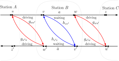
Figure 1: The event-activity network for a conflict on a single track. One train is driving from station A to station C while another train is driving in the opposite direction. The nodes represent the corresponding departure and arrival events and $a,\tilde{a}$ the waiting activities. Furthermore the disjunctive headway activities are shown, denoted by the variable name of corresponding constraint of the IP.

Lemma 1.

The safety margin $S_{vv^{\prime}}$ for two trains driving in opposite directions that enter and leave a station on the same track should satisfy

$$S_{vv^{\prime}}>\tfrac{1}{2}\,\max\{(L^{max}_{wz}-L^{min}_{wz}),(L^{max}_{uv}-L^{min}_{uv})\}.$$

Proof.

The event activity network for two trains, driving through a station in opposite directions on a single track is shown in Figure 1. In this case, we have $y_{a}=y_{\tilde{a}}=1$, i.e., the solution contains these conflicting trips. To simplify notation, we set $\pi_{v}^{*}=\pi_{v}+x_{v}$ for all $v\in\mathcal{E}$, and we use the new times of a dispatching timetable. In order to obtain a feasible timetable, the headway variables $g_{uw^{\prime}}$, $h_{vv^{\prime}}$, $g_{wu^{\prime}}$ should be equal. We show that

$$S_{vv^{\prime}}>\tfrac{1}{2}\,\max\{(L^{max}_{wz}-L^{min}_{wz}),(L^{max}_{uv}-L^{min}_{uv})\}$$

implies $g_{uw^{\prime}}=h_{vv^{\prime}}=g_{wu^{\prime}}=1$.

1. $h_{vv^{\prime}}=1\hskip 5.69054pt\Rightarrow\hskip 5.69054ptg_{wu^{\prime}}=1$
   If $h_{vv^{\prime}}=1$ then $\pi_{w}^{*}+S_{vv^{\prime}}<\pi_{v^{\prime}}^{*}$, because of (6). We have $L_{u^{\prime}w}=S_{u^{\prime}w}+L^{max}_{u^{\prime}v^{\prime}}=S_{vv^{\prime}}+L^{max}_{u^{\prime}v^{\prime}}$. If $g_{wu^{\prime}}=0$, it follows that

   $$\pi_{w}^{*} \geq\pi_{u^{\prime}}^{*}+L_{u^{\prime}v^{\prime}}^{min}+S_{vv^{\prime}}$$

   $$\pi_{w}^{*}+S_{vv^{\prime}} \geq\pi_{u^{\prime}}^{*}+L_{u^{\prime}v^{\prime}}^{min}+2S_{vv^{\prime}}$$

   $$\pi_{v^{\prime}}^{*} \geq\pi_{u^{\prime}}^{*}+L_{u^{\prime}v^{\prime}}^{min}+2S_{vv^{\prime}}$$

   $$\pi_{v^{\prime}}^{*}+L_{u^{\prime}v^{\prime}}^{max} \geq\pi_{u^{\prime}}^{*}+L_{u^{\prime}v^{\prime}}^{max}+L_{u^{\prime}v^{\prime}}^{min}+2S_{vv^{\prime}}\geq\pi_{v^{\prime}}^{*}+L_{u^{\prime}v^{\prime}}^{min}+2S_{vv^{\prime}}$$

   $$L_{u^{\prime}v^{\prime}}^{max} \geq L_{u^{\prime}v^{\prime}}^{min}+2S_{vv^{\prime}}$$

   $$S_{vv^{\prime}} \leq\tfrac{1}{2}\,(L_{u^{\prime}v^{\prime}}^{max}-L_{u^{\prime}v^{\prime}}^{min}),$$

   which is in contradiction to the condition on $S_{vv^{\prime}}$.

2. $g_{wu^{\prime}}=1\hskip 5.69054pt\Rightarrow\hskip 5.69054pth_{vv^{\prime}}=1$
   Assume $g_{wu^{\prime}}=1$ and $h_{vv^{\prime}}=0$. Because of (4), we have $\pi_{u^{\prime}}^{*}\geq\pi_{w}^{*}+L_{wz}^{min}+S_{vv^{\prime}}$. Because of (6) and $h_{vv^{\prime}}=0$, it follows that $\pi_{u^{\prime}}^{*}\geq\pi_{v^{\prime}}^{*}+S_{vv^{\prime}}+L_{wz}^{min}+S_{vv^{\prime}}$, which is in contradiction to the condition of $S_{vv^{\prime}}>0$.

3. $h_{vv^{\prime}}=1\hskip 5.69054pt\Rightarrow\hskip 5.69054ptg_{uw^{\prime}}=1$ and

4. $g_{uw^{\prime}}=1\hskip 5.69054pt\Rightarrow\hskip 5.69054pth_{vv^{\prime}}=1$ can be shown analogously. $\Box$

∎

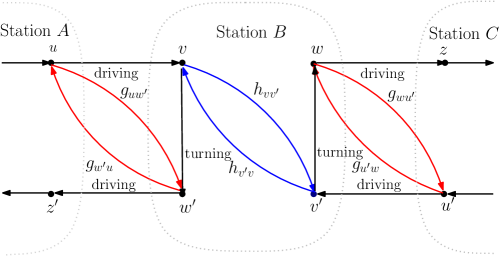
Figure 2: Example: Trains are allowed to turn at $B$

Remember that we cannot always express the headway constraints via a single variable, as the condition $g_{uw^{\prime}}=h_{vv^{\prime}}=g_{wu^{\prime}}$ does not hold, if trains are allowed to turn (see Figure 2).

As we described above, a flow model is integrated to model the circulation of trains. Constraint (8) ensures flow conservation on the events, i.e., the outflow should be equal to the inflow. A flow in the network encodes the sequence of trips for each train during the observed time interval. Note that trains represent a single commodity. Depots can consume flow (9) and initiate flow (10) with respect to the maximum number of replacement trains $R^{D_{i}}$ of depot $D_{i}\in\mathcal{D}$.

The big-$M$ has to be chosen sufficiently large in order to yield a correct model; analogous to [6], we set

$$M:=Y+\max_{(v,w)\in\mathcal{A}}(\pi_{w}-\pi_{v}+L_{vw}+S_{vw}),$$

where $Y$ denotes the maximum allowed delay for each event and we let $L_{vw}=S_{vv^{\prime}}=0$, on arcs where they have not been defined. In our case $Y$ is bounded by the cycle time.

We summarize:

Observation 1.

Feasible dispatching timetables $\pi^{\ast}=\pi+x$ correspond precisely to the feasible solutions of the integer program with constraints (2)–(14).

3.3 Reducing the Size of the Integer Program

The computational running time for solving the IP is mainly influenced by the number of precedence constraints in the system. These constraints involve big-$M$ constants and thus lead to a weak LP relaxation: here we can set each $g_{a}$ and $h_{a}$ with $a\in\mathcal{A}_{\text{head}}$ to $\tfrac{1}{2}$. This makes it desirable to reduce the number of precedence constraints by fixing them wherever possible. This can be achieved by considering the scheduling logic inherent in the system. If a disruption occurs, decisions for parts of the network imply decisions for other parts, e.g., if there are alternating sequences of driving and waiting activities with no turning possibilities. Furthermore, trains driving into the same direction cannot pass each other. Thus, variables can be fixed by using the natural precedence relations. In a second step, we can build blocks of such sequences and contract the driving and waiting activities into just one driving activity with the new minimum driving time. Because the delay of an event is passed to successive events, the travel time is bounded by the maximum allowed delay with respect to the buffer times. Safety intervals are inherited from the original event-activity network. The cost of the departure events is set to the sum of the corresponding contracted departure events. This process yields a reduced event-activity network $\mathcal{N}^{r}=(\mathcal{E}^{r},\mathcal{A}^{r})$.

Lemma 2.

An instance of the reduced network $\mathcal{N}^{r}=(\mathcal{E}^{r},\mathcal{A}^{r})$ has a feasible solution, if and only if the corresponding instance of the original event-activity network $\mathcal{N}=(\mathcal{E},\mathcal{A})$ has a feasible solution, and their objectives are equal.

Proof.

Let $\pi^{r}$ be a feasible dispatching timetable for the reduced event-activity network $\mathcal{N}^{r}=(\mathcal{E}^{r},\mathcal{A}^{r})$. Let $a=(v,w)\in\mathcal{A}^{r}$ be a driving activity, and let $\mathcal{E}_{\text{seq}}^{vw}\subset\mathcal{E}_{\text{dep}}\cup\mathcal{E}_{\text{arr}}$ be the corresponding sequence of events from the start event $v\in\mathcal{E}_{\text{dep}}$ to the end event $w\in\mathcal{E}_{\text{arr}}$. If $x_{v}\geq x_{w}$ in $\mathcal{N}^{r}$, we reduce the delay of the events along the sequence as late as possible; this is necessary to prevent blocking of following trains. If $x_{v}\leq x_{w}$, we increase the delay as soon as possible to prevent a collision with the train in front. The other direction follows analogously. $\Box$ ∎

Note that the overall delay of a dispatching in the the original network $\mathcal{N}$ that results from the application of the strategy in the above proof might be higher than the minimal possible delay in $\mathcal{N}$. This imposes no serious restriction, since our objective is insensitive to delays.

The reduced network $\mathcal{N}^{r}$ usually contains significantly fewer nodes and arcs, resulting in a smaller IP instance. This enables us to obtain solutions for significantly larger networks; in our experiments, the number of binary variables was reduced by roughly a factor of three.

4 Experiments

In this section we report on computational experiments, which we conducted to evaluate the applicability of our models. They are based on the real-life timetable of the subway line U6 in Vienna (Figure 3). We employed the Falko tool of Siemens AG [25]. Timetables are given with a granularity of one second.

The considered subway line has 24 stations, with terminal stations Siebenhirten and Floridsdorf; the regular travel time between these terminals is 34 minutes. We use typical frequencies of 5 or 10 minutes in our experiments. Trains are circulating between the terminals. The stations Floridsdorf, Michelbeuern, and Alterlaa are connected to depots that each contain a reserve train in our scenarios. Sidings exist at Siebenhirten. Our initial timetable contains buffer times of about 10% of the scheduled driving times between stations and at the end of the line.

We consider a variety of different disruptions with focus on the blockage of one side of the two tracks. Such disruptions often yield very hard instances and lead to severe problems in the daily operation of a line. During a disruption, a section of tracks on one side is blocked for a time interval between 5 minutes and 2 hours; until the section is reopened, no train is allowed to enter the blocked section. The track topology allows switching the track and performing a turn at several stations. Trips affected by the blocked section can use the unblocked track in the opposite direction. More specifically, we allow trains to pass the switches that are immediately before and after the blocked section. The circulation of a train can be truncated by introducing a turning.

For each scenario below, we use our model to generate a feasible dispatching timetable. We have to return to the original timetable within 60 minutes after reopening the blocked sections. Choices for trains include turning at specified stations, increasing their delays, or returning to a depot; the maximum allowed delay of a trip is equal to the cycle time.

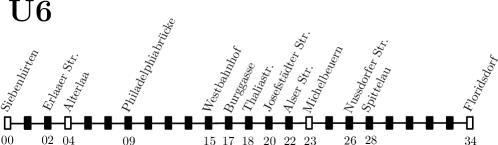
Figure 3: The Vienna subway line U6. Boxes represent the stations: a white box, if the station is connected to a depot or siding. The numbers below are the driving times from Siebenhirten to the stations.

4.1 Results

We tested four scenarios on the Vienna U6 that differ in location, transit times, the topology of the switches and turn possibilities to evaluate the impact of disruptions:

Scenario 1:

A disruption occurs between Michelbeuern and Westbahnhof. These stations are located close to the center of the line and are heavily used. Trips between these stations are assigned to the opposite track. Trains running from Michelbeuern to Westbahnhof have to switch the track after Michelbeuern and return to their originally assigned track between Burggasse and Westbahnhof. We allow trains to turn at Michelbeuern and Westbahnhof. The driving time between these stations is about 7 minutes and the trains have to share the same track in 4 stations.

Scenario 2:

A disruption occurs between Philadelphiabrücke and Erlaaer Straße that are located near the terminal station Siebenhirten. Trains have to switch the track in front of the station Philadelphiabrücke and back again before arriving at Erlaaer Straße. We allow trains to turn at these stations. The driving time is 7 minutes and the trains share the same track in 4 stations. The depot Alterlaa is located between those stations.

Scenario 3:

A disruption occurs between Nußdorfer Straße and Michelbeuern. Trains have to switch shortly after Nußdorfer Straße and return to their original track before arriving at Michelbeuern. Options for turning are given at Michelbeuern and (for trains going to Floridsdorf) after Spittelau. The driving time through the bottleneck is 3 minutes but points for turning are not close to the bottleneck section.

Scenario 4:

Here, a disruption occurs between Alser Straße and Thaliastraße, so that trains have to switch the track after Michelbeuern and return after Josephstädter Straße. The driving time between these stations is 5 minutes and the options for turning are given at Michelbeuern and Westbahnhof, which are not close to the disrupted track section.

For our experiments, we used the IP solver CPLEX 12.1 on a PC with a 3.0 GHz Intel Core2Duo CPU and 2 Gbytes of RAM.

The tables 1 – 6 are organized by scenarios and cycle frequencies; rows correspond to disruption times in minutes, indicated in the first column. Columns 2 shows the number of binaries that correspond to the precedence constraints and the flow on the activity arcs. All computations were performed using the reduced network. Column 3 gives the number of general variables for the delays. The fourth column shows the original number of trips in the undisrupted timetable during the observed time window. Column 5 shows the number of trips in the new dispatching timetable, derived with CPLEX in a maximum runtime of 1800 seconds, while the sixth column provides the best bound provided by CPLEX. Column 7 shows the necessary solution time in seconds, or (in case of delays of 45 minutes or more) 1800 if CPLEX could not establish optimality of a solution withing 1800 seconds. Column 8 indicates whether optimality could be proved, or the gap with respect to an upper bound. The final column 9 shows the number of trips in the disposition timetable, if we stop CPLEX finding a solution in only 60 seconds and succeed in finding at least a feasible solution. For this computation, the MIP node selection strategy of CPLEX is set to best estimate search.

Table 1: Scenario 1: disruption between Michelbeuern and Westbahnhof, cycle time of 5 minutes

dur	bin	int	$|\mathcal{A}_{dep}|$	sol	u.bound	time	status	60s
5	628	306	171	165	165.00	0.25	opt	165
10	745	331	177	171	171.00	3.41	opt	171
15	861	356	198	183	183.00	0.87	opt	183
20	978	381	207	189	189.00	9.42	opt	189
30	1215	431	231	207	207.00	24.88	opt	207
45	1578	506	267	231	231.00	141.56	opt	228
60	950	581	303	252	269.63	1800	7.0%	252
90	2721	731	375	276	351.14	1800	27.2%	–
120	3528	881	447	–	424.62	1800	–	–

Table 2: Scenario 1: disruption between Michelbeuern and Westbahnhof, cycle time of 10 Minutes

dur	bin	int	$|\mathcal{A}_{dep}|$	sol	u.bound	time	status	60s
5	254	150	85	85	85.00	0.08	opt	85
10	307	164	92	92	92.00	0.09	opt	92
15	365	175	97	97	97.00	0.89	opt	97
20	416	189	104	104	104.00	0.13	opt	104
30	524	214	116	110	110.00	4.04	opt	110
45	694	250	133	127	127.00	231.72	opt	127
60	854	289	152	146	146.00	559.87	opt	140
90	1193	364	188	170	188.00	1800	10.5%	170
120	1453	439	224	200	224.00	1800	12.0%	197

Table 3: Scenario 2: disruption between Philadelphiabrücke and Erlaaer Str., cycle time of 5 Minutes

dur	bin	int	$|\mathcal{A}_{dep}|$	sol	u.bound	time	status	60s
5	819	327	172	162	169.00	1.51	opt	162
10	913	353	184	184	184.00	0.28	opt	184
15	1092	379	196	183	183.00	5.30	opt	183
20	1231	405	208	192	192.00	7.64	opt	192
30	1515	457	232	209	209.00	59.11	opt	209
45	1956	535	268	236	243.00	1800	2.9%	235
60	2415	613	685	258	284.31	1800	10.2%	252
90	2721	731	375	276	351.14	1800	27.2%	272
120	3528	881	447	–	424.62	1800	–	–

Table 4: Scenario 2: disruption between Philadelphiabrücke and Erlaaer Str., cycle time of 10 Minutes

dur	bin	int	$|\mathcal{A}_{dep}|$	sol	u.bound	time	status	60s
5	348	158	86	86	86.00	0.08	opt	86
10	411	177	92	92	92.00	0.09	opt	92
15	473	184	98	98	98.00	0.14	opt	98
20	511	203	104	104	104.00	0.90	opt	104
30	623	229	116	116	116.00	0.12	opt	116
45	863	262	134	130	130.00	24.65	opt	130
60	1065	307	152	146	146.00	591.15	opt	145
90	1482	385	188	180	184.87	1800	2.7%	174
120	1917	463	224	209	221.00	1800	5.7%	209

Table 5: Scenario 3: disruption between Nußdorfer Straße and Michelbeuern, cycle time of 5 Minutes

dur	bin	int	$|\mathcal{A}_{dep}|$	sol	u.bound	time	status	60s
5	786	431	224	224	224.00	0.19	opt	224
10	891	462	238	233	233.00	0.77	opt	233
15	999	393	252	247	247.00	2.12	opt	247
20	1109	524	266	261	261.00	3.00	opt	261
30	1335	568	294	282	282.00	158.54	opt	283
45	1698	679	336	317	330.00	1800	4.1%	330
60	2061	772	378	352	372.00	1800	5.6%	372
90	2859	958	462	411	462.00	1800	12.4%	462
120	3729	1114	546	467	546.00	1800	16.9%	546

Table 6: Scenario 4: disruption between Alser Straße and Thaliastraße, cycle time of 5 Minutes

dur	bin	int	$|\mathcal{A}_{dep}|$	sol	u.bound	time	status	60s
5	798	416	224	224	224.00	0.17	opt	224
10	935	450	240	232	232.00	3.16	opt	232
15	1072	484	256	238	238.00	97.90	opt	238
20	1211	518	272	254	254.00	71.65	opt	272
30	1495	586	304	276	293.12	1800	6.7%	276
45	1936	688	352	316	343.96	1800	8.8%	316
60	2395	790	425	351	398.00	1800	13.6%	338
90	3367	994	496	419	495.22	1800	18.1%	–
120	4441	1198	592	481	592.00	1800	23.0%	–

4.2 Observations

We were able to find feasible solutions for most of the instances, including the relatively difficult scenarios with long disruption times. In most cases, these solutions were achieved quickly, while the bulk of the work was invested in establishing optimality. This indicates that our method should be suitable in even larger real-life situations in which a fast solution is needed and proving its optimality is a secondary concern. As described above, the LP relaxation is weak. Indeed, it has a large gap compared to the IP formulation. As a consequence the upper bounds are improved late during the solution process. If these bounds become more important, it may be of interest to establish additional inequalities.

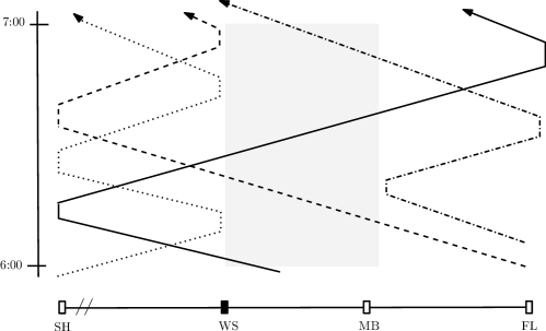
Figure 4: An excerpt of the time and space diagram of a new dispatching timetable. The diagram shows 4 trains circulating between the terminal stations Siebenhirten (SH) and Floridsdorf (FL). Due to a disruption between 6.00 a.m. and 7.00 a.m. only one track between Westbahnhof (WS) and Michelbeuern (MB) can be used. Thus, the schedules of the trains represented by the dashed and dotted lines become modified.

For practical purposes, the actual structure of the resulting vehicle schedules is of interest. An excerpt of a time and space diagram for the re-optimized timetable and vehicle schedule for a disruption of 60 minutes in Scenario 1 is shown in Figure 4.

The utilization of the tracks is generally high. But in the computed solutions, trains are still passing through the bottleneck section. The frequency, however, is heavily decreased. The new vehicle schedule contains 20 early turn operations. All of the three replacement trains are used, in order to realize the new timetable.

4.3 Extensions

Every change in the vehicle schedule needs to be distributed quickly to the involved persons. Furthermore, truncated circulations, caused by early turns or vehicles returning early to a depot, lead to necessary transfers for the passengers. Thus, it is desired to keep the number of transfers in the vehicle schedule reasonably low. To achieve this, we add a second term to the objective function by penalizing early turns and early returns to a depot:

$$\max\sum_{v\in\mathcal{E}_{\text{dep}}}\sum_{a\in\delta^{+}(v)}c_{a}\,y_{a}-\sum_{b\in\mathcal{A}_{\text{turn}}\cup\mathcal{A}_{\text{return}}}c_{b}\,y_{b}.$$ (15)

Each unplanned turning or early return to a depot penalizes the objective value by $c_{b}$. This results in a trade-off between the number of recovered weighted trips and the transfers for passengers.

In first experiments, we were able to find solutions with significantly less transfers for the passengers, but only a few more canceled trips. Fine tuning the weight coefficients $c_{a}$ and $c_{b}$ is important, since they have big impact on the design of the circulations provided by solution.

We are optimistic that the interaction with practitioners may help in designing better models, with preferences for particular solution types. For example, if the minimal transfer time of the disrupted section is quite small compared to the cycle frequency, delaying the affected trips could be sufficient. Furthermore, computed solutions often have an alternating structure: the disposition timetable often builds clusters of trips (with respect to their safety distance) and let these clusters alternate through the bottleneck. On the other hand, if the transfer time is too large, just delaying trips is not sufficient, trips have to be dropped and the solutions often contain shuttle trains. Finally, allowing trains to turn within the bottleneck yields some good solutions.

5 Conclusions

We have introduced techniques for integrated rescheduling of trips and vehicles for real-time disruption management of rail-based public transportation systems, especially for subway systems. Using an IP formulation and appropriate reduction techniques, we were able to achieve very good solutions for a variety of test scenarios arising from a real-world subway line. Tests show that our feasible solutions are always optimal or close to being optimal, indicating the practical usefulness of our method.

The spectrum of further improvements includes fine-tuning of our IP/LP approach and exploiting the structure of the underlying networks to reduce the solution space in advance. We would like to deal with larger-scale networks, for examples (subway) systems that do not have separated track system for each line.

References

- [1] Jespersen-Groth, J., Potthoff, D., Clausen, J., Huisman, D., Kroon, L. G., Maróti, G., and Nielsen, M. N., 2009. “Disruption management in passenger railway transportation”. In Robust and Online Large-Scale Optimization, R. K. Ahuja, R. H. Möhring, and C. D. Zaroliagis, eds., Vol. 5868 of Lecture Notes in Computer Science. Springer, pp. 399–421.
- [2] Liebchen, C., 2006. “Periodic timetable optimization in public transport”. Dissertation, TU Berlin.
- [3] Schöbel, A., 2001. “A model for the delay management problem based on mixed-integer programming”. Electronic Notes in Theoretical Computer Science, 50(1).
- [4] Schöbel, A., 2007. “Integer programming approaches for solving the delay management problem”. In Algorithmic Methods for Railway Optimization, no. 4359 in Lecture Notes in Computer Science. Springer, pp. 145–170.
- [5] Schachtebeck, M., and Schöbel, A., 2008. “IP-based techniques for delay management with priority decisions”. In ATMOS 2008 – 8th Workshop on Algorithmic Approaches for Transportation Modeling, Optimization, and Systems, M. Fischetti and P. Widmayer, eds., Schloss Dagstuhl. http://drops.dagstuhl.de/opus/volltexte/2008/1586.
- [6] Schachtebeck, M., 2009. “Delay management in public transportation: Capacities, robustness, and integration”. Dissertation, Universität Göttingen.
- [7] Gatto, M., Jacob, R., Peeters, L., and Schöbel, A., 2005. “The computational complexity of delay management”. In Graph-Theoretic Concepts in Computer Science: 31st International Workshop, WG 2005, D. Kratsch, ed., Vol. 3787 of Lecture Notes in Computer Science.
- [8] Caprara, A., Fischetti, M., and Toth, P., 2002. “Modeling and solving the train timetabling problem”. Operations Research, 50(5), pp. 851–861.
- [9] Hofman, M., Madsen, L., Groth, J. J., Clausen, J., and Larsen, J., 2006. “Robustness and recovery in train scheduling – a case study from DSB S-tog a/s”. In ATMOS 2006 – 6th Workshop on Algorithmic Methods and Models for Optimization of Railways, R. Jacob and M. Müller-Hannemann, eds., Schloss Dagstuhl. http://drops.dagstuhl.de/opus/volltexte/2006/687.
- [10] Biederbick, C., and Suhl, L., 2004. “Decision support tools for customer-oriented dispatching”. In ATMOS, F. Geraets, L. G. Kroon, A. Schöbel, D. Wagner, and C. D. Zaroliagis, eds., Vol. 4359 of Lecture Notes in Computer Science, Springer, pp. 171–183.
- [11] Gely, L., Feillee, D., and Dessagne, G., 2009. A cooperative framework between optimization and simulation to adress on-line re-scheduling problems. Tech. Rep. 178, ARRIVAL project.
- [12] Törnquist, J., 2006. “Computer-based decision support for railway traffic scheduling and dispatching: A review of models and algorithms”. In 5th Workshop on Algorithmic Methods and Models for Optimization of Railways, L. G. Kroon and R. H. Möhring, eds., Schloss Dagstuhl. http://drops.dagstuhl.de/opus/volltexte/2006/659.
- [13] Törnquist, J., and Persson, J. A., 2007. “N-tracked railway traffic re-scheduling during disturbances”. Transportation Research Part B: Methodological, 41(3), pp. 342–362.
- [14] Gatto, M., and Widmayer, P., 2007. On Robust Online Job Shop Scheduling. Tech. Rep. 62, ARRIVAL Project.
- [15] Nielsen, L. K., 2008. A Decision Support Framework for Rolling Stock Rescheduling. Tech. Rep. 158, ARRIVAL Project.
- [16] Borndörfer, R., and Schlechte, T., 2007. “Solving railway track allocation problems”. In Operations Research Proceedings 2007, J. Kalcsics and S. Nickel, eds., pp. 117–122.
- [17] Cacchiani, V., Caprara, A., and Toth, P., 2008. “A column generation approach to train timetabling on a corridor”. 4OR, 6(2), pp. 125–142.
- [18] Huisman, D., 2007. “A column generation approach for the rail crew re-scheduling problem”. European Journal of Operational Research, 180(1), pp. 163–173.
- [19] Veelenturf, L., Potthoff, D., Huisman, D., and Kroon, L., 2009. Railway crew rescheduling with retiming. Econometric Institute Report EI 2009-24, Erasmus University Rotterdam, Econometric Institute. http://ideas.repec.org/p/dgr/eureir/1765016746.html.
- [20] Clausen, J., Larsen, A., Larsen, J., and Rezanova, N. J., 2010. “Disruption management in the airline industry–concepts, models and methods”. Computers and Operations Research, 37(5), pp. 809–821.
- [21] Liebchen, C., 2008. “Linien-, Fahrplan-, Umlauf- und Dienstplanoptimierung: Wie weit können diese bereits integriert werden?”. In Heureka ’08 – Optimierung in Transport und Verkehr, Tagungsbericht, M. Friedrich, ed., FGSV Verlag.
- [22] Serafini, P., and Ukovich, W., 1989. “A mathematical model for periodic scheduling problems”. SIAM Journal on Discrete Mathematics, 2(4), pp. 550–581.
- [23] Nachtigall, K., 1998. “Periodic network optimization and fixed interval timetables”. Habilitationsschrift, Deutsches Zentrum für Luft- und Raumfahrt, Institut für Flugführung, Braunschweig.
- [24] Opitz, J., 2009. “Automatische Erzeugung und Optimierung von Taktfahrplänen in Schienenverkehrsnetzen”. Dissertation, Technische Universität Dresden.
- [25] K.-H. Erhard, Y. Schmidtke, H. S., 2000. “Falko: Fahrplan-validierung und -konstruktion für spurgebundene verkehrssysteme”. Signal+Draht, 92.