Analog of Electromagnetically Induced Transparency Effect for Two Nano/Micro-mechanical Resonators Coupled With Spin Ensemble

Abstract

We study a hybrid nano-mechanical system coupled to a spin ensemble as a quantum simulator to favor a quantum interference effect, the electromagnetically induced transparency (EIT). This system consists of two nano-mechanical resonators (NAMRs), each of which coupled to a nuclear spin ensemble. It could be regarded as a crucial element in the quantum network of NAMR arrays coupled to spin ensembles. Here, the nuclear spin ensembles behave as a long-lived transducer to store and transfer the NAMRs’ quantum information. This system shows the analog of EIT effect under the driving of a probe microwave field. The double-EIT phenomenon emerges in the large $N$ (the number of the nuclei) limit with low excitation approximation, because the interactions between the spin ensemble and the two NAMRs are reduced to the coupling of three harmonic oscillators. Furthermore, the group velocity is reduced in the two absorption windows.

I Introduction

In quantum information, an important task is the long-lived storage and remote quantum state transfer inf ; cirac ; bennet ; shi1 ; shi2 of quantum information. There exist several approaches to the implementation of quantum storage, such as electromagnetically induced transparency (EIT) based on three-level atomic ensemble harris ; hau ; scully ; lukin ; lukin1 ; lukin2 ; hau1 ; liyong ; liyong1 , nuclear spins coupled to electrons zhangp , and polarized molecular ensembles coupled to cavity fields in superconducting transmission lines zhou ; liao1 ; liao2 . Nuclear spin ensemble has the advantage that its transverse relaxation time $T_{2}$ can reach a second time scale lukin3 ; t2 . In earlier works lukin3 ; zoller2 ; poggio1 ; zhangp , the nuclei ensemble has been used to store the quantum information of electron spins, since the electron spin’s decoherence time $T_{e2}$ is in the order of ten milliseconds t2 ; te2 , which is much shorter than the nuclear spins’ relaxation time.

Recently, the optomechanical systems containing micro/nano-mechanical resonators have inspired extensive studies in many aspects, such as the entanglements of the mechanical resonators with the light mancini ; knight ; penrose ; vitali , and even the atoms vitali1 ; ian ; chang , cooling the mechanical resonators through light pressure meystre0 ; meystre ; meystre1 ; vitali2 ; zoller0 , and the nonclassical states in the hybrid system knight1 ; gong ; zoller1 . In fact, the micro/nano-mechanical resonator’s decoherence time $T_{r2}$ is shorter tr20 ; tr2 ($\sim$100 $\mu$s) than the life time of the nuclear spins. Therefore, it is expect to store the information of the micro/nano-mechanical resonator in the nuclear spins. Actually, the coupling between the nuclear spin ensemble (or a single spin) and the mechanical resonator tips has drawn much attention rugar ; sidles ; rugar1 ; rugar2 ; rugar3 ; rugar4 ; rugar5 ; xuef both in theories and in experiments. An important innovation based on the coupling of single/few spins to the mechanical tip is the magnetic resonance force microscopy (MRFM) rugar ; sidles ; rugar1 ; rugar2 ; rugar3 ; rugar4 ; rugar5 ; poggio . MRFM uses a cantilever tipped with a ferromagnetic particle producing a inhomogeneous magnetic field that couples the mechanical tip to the sample spins. By measuring the displacement of the tip with an interferometer, a series of 2-D images of the spin sample is acquired mri . In practice, the spin sample is usually a spin ensemble containing a lot of electrons or nuclear spins, which could be excited to show the collective behavior. Such collective motion could achieve the effective strong coupling to the nano-mechanical resonator (NAMR).

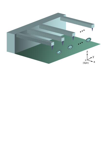
Figure 1: (Color online) Schematic setup of the NAMR-spin-NAMR-… system. Here, the spin ensembles are placed between two nearest NAMRs in the NAMR array, and each of the NAMR has a tiny ferromagnetic particle in the mechanical tip. The spin ensembles behave as a transducer that store the NAMRs’ quantum information and transfer them from one NAMR to the next one.

With the above mentioned investigations about various hybrid systems concerning the nuclear spin ensembles and NAMRs, Rabl et.al. lukin4 explore the possibility of using the short life time NAMR as a quantum data bus for spin quibit coupled to magnetized mechanical tips, and the mechanical resonators are coupled through Coulomb forces. This study motivates us to utilize the nuclear spin ensemble itself as long-lived data bus (the spin ensemble also behaves as a quantum transducer liu ) to realize the effective couplings among the NAMRs. The advantage of our proposal is that the quantum transducer has the life time much longer than the NAMR’s. Our setup is shown in Fig. 1, where an array of NAMRs is coupled to nuclear spin ensembles, which are placed between the nearest two tips. Each spin ensemble induces interaction between the corresponding tips, and the quantum information of the tips can be transferred from one to the another one by one. This dynamic process realizing the quantum information transfer physically depends on an controllable coupling among the three systems, two NAMRs and a spin ensemble. We will show that the double EIT effect exists in our present setup, which plays an important role in the coherent storage of quantum information in this hybrid-element sub-system.

In the conventional EIT effect based on the $\Lambda$-type three-level atomic ensemble on two-photon resonance, a driving light suppresses the absorption of another light (the probe light), and even makes the probe light transparent at the frequency at which the probe light should be absorbed strongly without the driving field scully1 . An important physical mechanism in this EIT effect is that the pump light induces an ac-Stark splitting of the excited state. As a result, the probe light is off-resonant with the energy spacing of the energy levels it couples to. Actually, the EIT effect analog exists in a system of two coupled harmonic oscillators one of which is subject to a harmonic driving force alzar . In fact, the coupling between the two harmonic oscillators will change their original frequencies, and make the absorbed power deviate from resonance. This reason is similar to that in the conventional EIT phenomenon. We show that our proposed setup consisting of a magnetized mechanical tip coupled to a nuclear ensemble, which behaves as a two coupled harmonic oscillator system, can also exhibit the phenomenon similar to the EIT effect in the system with light-atom interaction.

We will study in details the double EIT effect analog in a sub-network of the whole structure shown in Fig. 1, a NAMR-spin ensemble-NAMR coupling system. In the low excitation limit with large $N$ (the number of the nuclear spins) limit, the spin excitation behaves as a single mode boson liyong1 ; zhangp ; ian coupled respectively to the two mechanical tips. In this case, the interaction between the spins and each tip is the coupling between two harmonic oscillators with effective amplified strength proportional to $\sqrt{N}$. In general, this three oscillator-coupling system have three eigen-frequencies (taking account of the degeneracy). And we show that there are two absorption windows for the probe microwave field, with the absorption peaks corresponding to the three eigen-frequencies. In these two windows with normal dispersion relations, the group velocity of the microwave field is reduced dramatically. These transparency and slow light phenomena correspond to EIT effect.

The paper is organized as follows: in Sec. II, we illustrate the sub-network composed of two nano-mechanical resonators coupled to a spin ensemble; in Sec. III, we study the mechanical analog of EIT effect in a NAMR-nuclear ensemble coupling system, and make a comparison with the AMO system by revisiting the conventional EIT phenomenon; in Sec. IV, we study the double-EIT effect in the sub-network hybrid system and show the slowing light phenomenon in Sec. V; in Sec. VI, we summarize our result.

II Setup and Modeling for Quantum Transducer

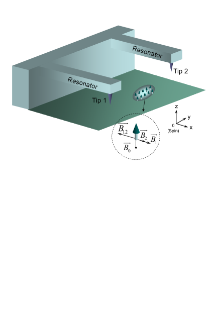
Figure 2: (Color online) Schematic setup of the NAMR-spin ensemble-NAMR coupling system. The ensemble of spins is placed between two NAMRs each of which has a tiny ferromagnetic particle in the tip. Both of the directions of the two magnetic field produced by the two tips are along the $x$-axis. The origin of the coordinate frame is at the center of the spin ensemble. The spin ensemble is also exposed in two static magnetic fields $\vec{B}_{12}$ along the $x$-axis, and $\vec{B}_{0}$ along the $z$-axis.

We now consider a hybrid system consisting of two NAMRs and a nuclear spin ensemble containing $N$ spins. This system is the basic unit for constructing the whole quantum network (Fig. 1). The spin-NAMR hybrid system is illustrated in Fig. 2. In this setup, each NAMR is coupled to the ensemble of $N$ $1/2$-spin particles by a tiny ferromagnetic particle attached to it. The origin of the reference frame is chosen to be the center of the nuclear spin ensemble. The NAMRs can oscillate in the $z$-direction, and each magnetized tip attached to the corresponding NAMR produces a dipolar magnetic field at the position of the spins as jackson

$$\vec{B}_{j}=\frac{\mu_{0}\left[3\left(\vec{m}_{j}\cdot\vec{n}_{j}\right)\vec{n}_{j}-\vec{m}_{j}\right]}{4\pi r_{j}^{3}},\text{ }j=1,2,$$ (1)

where $\mu_{0}$ is the vacuum magnetic conductance, $\vec{m}_{j}$ is the $j$the ferromagnetic particle’s magnetic moment, $\vec{n}_{j}$ is the corresponding unit vector pointing in the direction from the tip to the spin. Here, $r_{j}$, which varies due to the oscillation of the NAMR along the $z$-direction, is the distance between the magnetic tip and the spin. In our setup, both of the magnetic moments in the two tips are in the $x$-direction as $\vec{m}_{1}=m_{1}\hat{e}_{x}$ and $\vec{m}_{2}=m_{2}\hat{e}_{x}$. The equilibrium positions of the two NAMRs are $\vec{r}_{1}$ and $\vec{r}_{2}$ respectively, and both $\vec{r}_{1}$ and $\vec{r}_{2}$ are in the $yz$-plane. We have assumed that the spins are confined in a very small volume, and the magnetic fields produced by the two ferromagnetic particles at the spin ensemble are uniform as $\vec{B}_{1}=\left(B_{1}\left(z_{1}\right),0,0\right)$ and $\vec{B}_{2}=\left(B_{2}\left(z_{2}\right),0,0\right)$ respectively, where

$$B_{j}\left(z_{j}\right)\approx A_{j}-G_{j}z_{j}\text{, }j=1,2\text{,}$$ (2)

with $z_{1}\left(z_{2}\right)$ the small deviation of the tip1 (tip2) from the equilibrium position. Here, $A_{1}=-\mu_{0}m_{1}/\left(4\pi\left|\vec{r}_{1}\right|^{3}\right),$ $A_{2}=-\mu_{0}m_{2}/\left(4\pi\left|\vec{r}_{2}\right|^{3}\right)$, together with the magnetic field gradients

$$G_{1}=\frac{3r_{1z}\mu_{0}m_{2}}{4\pi\left|\vec{r}_{1}\right|^{5}}\text{, }G_{2}=\frac{3r_{2z}\mu_{0}m_{2}}{4\pi\left|\vec{r}_{2}\right|^{5}}\text{,}$$ (3)

where $r_{jz}=\vec{r}_{j}\cdot\hat{e}_{z}$, for $j=1,2$. Besides these two magnetic fields, the spins are also exposed to two static magnetic fields $\vec{B}_{12}=\left(-A_{1}-A_{2},0,0\right)$, and $\vec{B}_{0}=-B_{0}\hat{e}_{z}$. We note that in experiments rugar1 ; rugar2 ; mn , the distance between the magnetized tip and the nuclear ensemble is in the order of 100 nanometers, and the nuclear spin ensemble containing more than 100 nuclei is attached in a quantum dot with the diameter in 10 nanometers length scale. Thus the the magnetic field $B_{j}\left(z_{j}\right)$ is approximately homogeneous in the nuclear ensemble when $z_{j}$ is fixed.

Both of the NAMRs are described as harmonic oscillators with effective masses $M_{j}$ and frequencies $\omega_{j}$. Then the Hamiltonian $H_{0}^{d}$ of this spin-NAMRs coupling system is

$$H_{0}^{d} = \frac{p_{1}^{2}}{2M_{1}}+\frac{p_{2}^{2}}{2M_{2}}+\frac{1}{2}M_{1}\omega_{1}^{2}z_{1}^{2}+\frac{1}{2}M_{2}\omega_{2}^{2}z_{2}^{2}$$ (4)

$$+\sum_{j=1}^{N}\left(g_{1}\sigma_{j}^{x}z_{1}+g_{2}\sigma_{j}^{x}z_{2}+g_{0}\sigma_{j}^{z}\right),$$

where $p_{j}$ is the momentum of the NAMR $j$, $\sigma_{x}$ and $\sigma_{y}$ are Pauli matrixes describing the spin. Here, the spin-NAMR coupling strength $g_{j}=g_{s}\mu_{B}G_{j}/2$ for $j=1,2$, where $g_{s}$ is the g-factor of the spin, $\mu_{B}$ is the Bohr magneton, and $g_{0}=g_{s}\mu_{B}B_{0}/2.$ Note that the the first order in the magnetic dipole-dipole interaction

$$H_{d-d}=\frac{\mu_{0}\left[3\left(\vec{m}_{1}\cdot\hat{e}_{12}\right)\left(\vec{m}_{2}\cdot\hat{e}_{12}\right)-\vec{m}_{1}\cdot\vec{m}_{2}\right]}{4\pi\left|\vec{r}_{1}-\vec{r}_{2}\right|^{3}}$$ (5)

vanishes in our model, where $\hat{e}_{12}$ is the unit vector pointing in the direction from the tip1 to the tip2.

To see the analog of EIT effect, we apply a probe microwave field $\vec{B}_{\mathrm{p}}=-\hat{e}_{x}B_{\mathrm{p}}\cos\Omega t$ coupled to the spin ensemble. This coupling is described by the interacting Hamiltonian

$$H_{I}=\frac{1}{2}g_{s}\mu_{B}B_{\mathrm{p}}\cos\Omega t\sum_{j=1}^{N}\sigma_{j}^{x}.$$ (6)

The probe alternating magnetic field is similar to the probe light in the $\Lambda$-type atomic ensemble. The total Hamiltonian $H^{d}=H_{0}^{d}+H_{I}$ depicts the sub-network illustrated in Fig. 2.

When $N$ is large and with the low excitations of the spins, the excitations of the spins are described by two bosonic operators liyong1 ; zhangp ; ian

$$b=\frac{1}{\sqrt{N}}\sum_{j=1}^{N}\sigma_{j}^{-}$$ (7)

and its conjugate $b^{{\dagger}}$, where the commutation relation between $b$ and $b^{{\dagger}}$ is

$$\left[b,b^{{\dagger}}\right]\approx 1.$$ (8)

In terms of $b$ and $b^{{\dagger}}$ defined above, the Hamiltonian in Eq. (4) is rewritten as

$$H_{0}^{d} = \frac{\hbar\omega_{1}}{2}\left(P_{1}^{2}+Z_{1}^{2}\right)+\frac{\hbar\omega_{2}}{2}\left(P_{2}^{2}+Z_{2}^{2}\right)$$ (9)

$$+\frac{\hbar\omega_{0}}{2}\left(P_{0}^{2}+Z_{0}^{2}\right)+\hbar\sqrt{N}\sum_{j=1}^{2}G_{j}Z_{0}Z_{j}.$$

Here, we have defined the dimensionless operators

$$Z_{0}=\frac{b+b^{{\dagger}}}{\sqrt{2}},P_{0}=i\frac{b^{{\dagger}}-b}{\sqrt{2}},$$ (10)

$$Z_{j}=\sqrt{\frac{M_{j}\omega_{j}}{\hbar}}z_{j},P_{j}=\frac{p_{j}}{\sqrt{\hbar M_{j}\omega_{j}}},j=1,2.$$ (11)

The coupling constants $G_{j}=g_{j}\sqrt{2\hbar/M_{j}\omega_{j}}/\hbar,$ for $j=1,2$, and $\omega_{0}=2g_{0}/\hbar.$ In experiments, the parameters $\omega_{j}$ ($j=1,2$) and $\omega_{0}$ are in the order of 10⁶Hz, and$\ G_{j}\$can reach the order of $10^{5}Hz$.

Before the further investigations of the double-EIT effect in this hybrid system, we would like to show the mechanical analog of EIT phenomenon in a NAMR-spin ensemble coupling system with only a single NAMR, as the basic physics in the double-EIT phenomenon depends on the coherent coupling of the NAMR to the nuclear spin ensemble.

III Mechanical Analog of EIT

In this section, we show the analog of the EIT effect in the single NAMR coupled to a spin ensemble system. To this end, we will compare it with the EIT phenomenon in the AMO system.

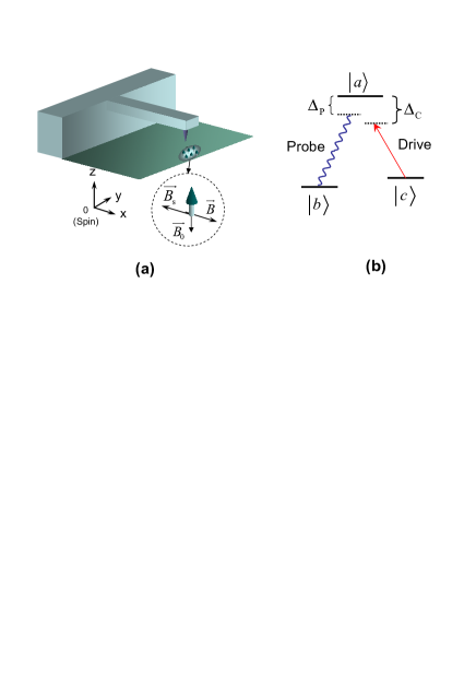
Figure 3: (Color online) The schematic of a NAMR couple to a spin ensemble [for (a)], and a $\Lambda$-type three-level atom [for (b)]. The EIT effect base on the atomic ensemble [for (b)] where each atom is coupled to a driving light and probe light has a analog in the two harmonic oscillator coupling system derived from the structure [for (a)]. In Fig (a), the spin ensemble is placed under the NAMR which has a tiny ferromagnetic particle in the tip. The direction of the magnetic field produced by the magnetized tip is along the $x$-axis. The origin of the coordinate frame is at the center of the spin ensemble. The spin ensemble is also exposed in two static magnetic fields $\vec{B}_{\mathrm{s}}$ along the $x$-axis, and $\vec{B}_{0}$ along the $z$-axis.

To reveal the basic physical mechanism, we first consider a system consisting of a nano-mechanical resonator (NAMR) and a nuclear spin ensemble containing $N$ spins. The spin-NAMR hybrid system is illustrated in Fig. 3(a). The origin of the reference frame is chosen to be the center of the nuclear spin ensemble. The NAMR can oscillate along the $z$-direction, and the magnetized tip attached to the NAMR produces a dipolar magnetic field at the position of the spin, with the magnetic field $\vec{B}=\left(B\left(z\right),0,0\right)$, where

$$B\left(z\right)\approx A-Gz\text{,}$$ (12)

with $A=-\mu_{0}m/\left(4\pi\left|\vec{r}\right|^{3}\right)$, and the magnetic field gradient is $G=3r_{z}\mu_{0}m/\left(4\pi\left|\vec{r}\right|^{5}\right).$ Here, $\vec{m}=m\hat{e}_{x}$ is the ferromagnetic particle’s magnetic moment, $\vec{n}$ is the unit vector pointing in the direction from the tip to the spin, and $\vec{r}$ in the $yz$-plane is the equilibrium position of the tip. We assume that the spins are confined in a very small volume. In the gradient $G$, $r_{z}=\vec{r}\cdot\hat{e}_{z}$. Besides the magnetic field $B\left(z\right)$ produced by the magnetized tip, the spins are also exposed to two static magnetic fields $\vec{B}_{s}=\left(-A,0,0\right)$, and $\vec{B}_{0}$.

The magnetized tip is described as a harmonic oscillator with the effective mass $M$ and frequency $\omega$. With a probe microwave field $\vec{B}_{\mathrm{p}}=-\hat{e}_{x}B_{\mathrm{p}}\cos\Omega t,$ the Hamiltonian $H$ of this spin-NAMR hybrid system is $H=H_{0}+H_{I}$, where

$$H_{0}=\frac{p^{2}}{2M}+\frac{1}{2}m\omega^{2}z^{2}+\sum_{j=1}^{N}\left(g\sigma_{j}^{x}z+g_{0}\sigma_{j}^{z}\right).$$ (13)

with $p$ the momentum of the NAMR. Here, the spin-NAMR coupling strength $g=g_{s}\mu_{B}G/2$.

Actually, when $N$ is large and with the low excitations of the spins, following the similar procedure to that in the last section, the Hamiltonian in Eq. (13) is rewritten as

$$H_{0} = \frac{\hbar\omega_{0}}{2}\left(P_{0}^{2}+Z_{0}^{2}\right)+\frac{\hbar\omega}{2}\left(P^{2}+Z^{2}\right)$$ (14)

$$+\hbar G\sqrt{N}Z_{0}Z,$$

where

$$Z=\sqrt{\frac{M\omega}{\hbar}}z,P=\frac{p}{\sqrt{\hbar M\omega}},$$ (15)

and the NAMR-spin ensemble coupling constant is $G=g\sqrt{2\hbar/m\omega}/\hbar$.

It is shown in Eq. (14) that under the low excitation approximation with large $N$ limit, the NAMR-spin ensemble coupling system is described by a two harmonic coupling system if $\omega_{0}>0$, with the coupling constant proportional to $\sqrt{N}$. In large $N$ limit with low excitations, $H_{I}$ is written as

$$H_{I}=\hbar\sqrt{N}G_{\mathrm{p}}Z_{0}\left(e^{-i\Omega t}+e^{i\Omega t}\right),$$ (16)

where $G_{\mathrm{p}}=g_{s}\mu_{B}B_{\mathrm{p}}/\left(\sqrt{2}\hbar\right)$. The set of Heisenberg-Langevin equations gives

$$\partial_{t}^{2}Z_{0} = -\gamma_{0}\dot{Z}_{0}-\omega_{0}^{2}Z_{0}-\omega_{0}\sqrt{N}GZ$$ (17)

$$-\omega_{0}\sqrt{N}G_{\mathrm{p}}\left(e^{-i\Omega t}+e^{-i\Omega t}\right),$$

$$\partial_{t}^{2}Z=-\gamma\dot{Z}-\omega^{2}Z-\omega\sqrt{N}GZ_{0},$$ (18)

where $\gamma_{0}$ ($\gamma$) is the decay rate for $Z_{0}$ ($Z$). The probe microwave field also provides a “driving” term in the set of equations (17) and (18), as what the probe light behaves in the conventional EIT phenomenon. Here, we have ignored the fluctuations as we are interested in the steady states and the fluctuations’ expectation values on the steady states are zero. The solutions to Eqs. (17) and (18) have the form

$$Z_{0s}\left(t\right)=Z_{0s}\left(\Omega\right)e^{-i\Omega t}+Z_{0s}\left(-\Omega\right)e^{i\Omega t},$$ (19)

and

$$Z_{s}\left(t\right)=Z_{s}\left(\Omega\right)e^{-i\Omega t}+Z_{s}\left(-\Omega\right)e^{i\Omega t}.$$ (20)

It follows from Eqs. (17)-(20) that the solution for $Z_{0s}\left(\Omega\right)$ is

$$Z_{0}\left(\Omega\right)=\frac{\omega_{0}\sqrt{N}G_{\mathrm{p}}\xi}{-N\omega_{0}\omega G^{2}+\xi_{0}\xi},$$ (21)

where

$$\xi_{0}=i\Omega\gamma_{0}-\omega_{0}^{2}+\Omega^{2},$$ (22)

and

$$\xi=i\Omega\gamma-\omega^{2}+\Omega^{2}.$$ (23)

The magnetic susceptibility of the alternating magnetic field $\vec{B}_{\mathrm{p}}$, $\chi_{M}$ is

$$\chi_{M}=\frac{\vec{M}}{\vec{B}_{\mathrm{p}}/\mu_{0}-\vec{M}}\approx\frac{\mu_{0}\vec{M}}{\vec{B}_{\mathrm{p}}},$$ (24)

where $\mu_{0}$ is the permeability of vacuum, and the magnetization intensity $\vec{M}$ is

$$\vec{M} = \hat{e}_{x}\frac{g_{s}\mu_{B}}{2}\left\langle\sum_{j=1}^{N}\sigma_{j}^{x}\right\rangle/V$$ (25)

$$= \hat{e}_{x}\frac{\sqrt{N}g_{s}\mu_{B}}{\sqrt{2}V}\left[Z_{0s}\left(\Omega\right)e^{-\mathrm{i}\Omega t}+\mathrm{c.c.}\right],$$

with the volume of the spin ensemble $V$. Here, we have assumed that the magnetization intensity $\left|\vec{M}\right|$ is small compared with $\left|\vec{B}_{\mathrm{p}}\right|/\mu_{0}$, in order to ensure the validity of the expansion in Eq. (24). Consequently, the magnetic susceptibility $\chi_{M}\left(\Omega\right)$ is

$$\chi_{M}\left(\Omega\right)=-\frac{\mu_{0}g_{s}\mu_{B}}{\sqrt{2}VB_{\mathrm{p}}}\sqrt{N}Z_{0s}\left(\Omega\right).$$ (26)

The real part and the imaginary part of $\chi_{M}\left(\Omega\right)$ depict the dispersive response and the absorption respectively. With the parameters as (in the unit of $\omega_{0}$) $\omega=1$, $\gamma_{0}=5\times 10^{-2}$, $\gamma=10^{-7}$, $G_{\mathrm{p}}=1$, $N=20$, $B_{\mathrm{p}}=\sqrt{2}\hbar G_{\mathrm{p}}/g_{s}\mu_{B}$, and $V=\left(4\pi/3\right)10^{3}\mathrm{nm}^{3}$, we plot Re[$\chi_{M}\left(\Omega\right)$] and Im[$\chi_{M}\left(\Omega\right)$] in Figs. 4(a) and 4(b), for $G=0$ and $G=0.05$ respectively. In Fig. 4(a), the absorbed peak is at the frequency $\Omega=\omega$, as the nuclear spin ensemble is decoupled with the NAMR. The absorption window and slow light phenomenon for the microwave field due to the coupling with the NAMR are illustrated in Fig. 4(b), which shows the analog of EIT. We note that there are two absorption peaks in Fig. 4(b), corresponding approximately to the two eigen-frequencies derived from Eq. (14). In the absorption window, the slope of Re[$\chi_{M}\left(\Omega\right)$] is positive, which illustrates that the group velocity of the microwave field is reduced dramatically.

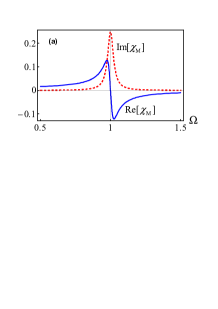
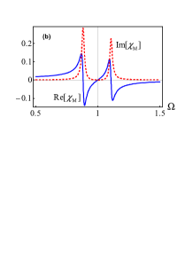
Figure 4: (Color online) The frequency dependence of the real part (the blue solid line) and the imaginary part (the red dashed line) of the susceptibility $\chi_{M}\left(\Omega\right)$ in single NARM-spin ensemble coupling system. The NAMR-spin coupling constant $G$ is: (a) $G=0$; (b) $G=0.05$. When The NAMR-spin coupling exists, there is a window in the absorption spectrum, with the positive slope of Re[$\chi_{M}\left(\Omega\right)$] in the window. This is an analog of EIT effect in the atomic ensemble.

To see why the above mechanical system can display an EIT analog and its intrinsic mechanism in detail, we revisit the EIT effect in an AMO system shown in Fig. 3(b). Fig. 3(b) shows the energy levels of the $\Lambda$-type atom of the atomic ensemble. Here, the single-mode driving field makes transition between the excited state $\left|a\right\rangle$ and the second lowest state $\left|c\right\rangle$ with the detuning $\Delta_{\mathrm{c}}=\omega_{\mathrm{ac}}-\nu_{\mathrm{c}}$, while the single-mode probe light makes transition between the state $\left|a\right\rangle$ and the lowest state $\left|c\right\rangle$ with the detuning $\Delta_{\mathrm{p}}=\omega_{\mathrm{ab}}-\nu_{\mathrm{p}}$. Here, $\omega_{\mathrm{ac}}$ ($\omega_{\mathrm{ab}}$) is the energy level spacing between the states $\left|a\right\rangle$ and $\left|c\right\rangle$ ($\left|b\right\rangle$), and $\nu_{\mathrm{c}}$ ($\nu_{\mathrm{p}}$) is the frequency of the driving (probe) light. In the rotating frame with respect to liyong1

$$\nu_{\mathrm{p}}S+\left(\omega_{\mathrm{ab}}-\omega_{\mathrm{ac}}\right)\sum_{j=1}^{N_{a}}\left|c\right\rangle_{jj}\left\langle c\right|+\nu_{\mathrm{p}}a^{{\dagger}}a,$$ (27)

in the large $N_{a}$ (the number of atoms) limit with low excitations of the atom ensemble, the Hamiltonian is

$$H_{EIT}=\Delta_{\mathrm{p}}A^{{\dagger}}A+\left(g_{\mathrm{p}}\sqrt{N_{a}}aA^{{\dagger}}+g_{\mathrm{c}}e^{\mathrm{i}\left(\Delta_{\mathrm{c}}-\Delta_{\mathrm{p}}\right)t}A^{{\dagger}}C+\mathrm{H.c.}\right),$$ (28)

where the atomic collective excitation are described by

$$A^{{\dagger}}=\frac{1}{\sqrt{N_{a}}}\sum_{j=1}^{N_{a}}\left|a\right\rangle_{jj}\left\langle b\right|,\text{ }C=\frac{1}{\sqrt{N_{a}}}\sum_{j=1}^{N_{a}}\left|b\right\rangle_{jj}\left\langle c\right|,$$ (29)

and the operators defined in Eqs. (29) satisfy the commutation relations approximately as liyong1 $\left[A,A^{{\dagger}}\right]\approx 1,$ $\left[C,A^{{\dagger}}\right]\approx 0,$ and $\left[C,C^{{\dagger}}\right]\approx 1.$ Here, $a$ ($a^{{\dagger}}$) is the annihilation (creation) operator of the probe light, and $\left|\alpha\right\rangle_{jj}\left\langle\beta\right|$ ($\alpha$, $\beta=a,b,c$) is $j$th atom’s flip operator. $g_{\mathrm{p}}$ ($g_{\mathrm{c}}$) is the coupling constant of the probe (driving) light and a single atom with the corresponding energy levels. We assume that both $g_{\mathrm{p}}$ and $g_{\mathrm{c}}$ are real. It is shown in Eq. (28) that the EIT effect based on the $\Lambda$-type three level atomic ensemble can be re-explained by the coupling of two “harmonic oscillators” (depicted by the collective excitation operators $A$ and $C$), with the coupling strength $g_{\mathrm{c}}$. Here, the coupling of $A$-mode to the quantized field of $a$ can compare with the semi-classical coupling in Eq. (14). Note that under the rotating-wave approximation, the Hamiltonian $H$ in Eqs. (14) and (16) has the same form as $H_{EIT}$ in Eq. (28). As a result, the hybrid system consisting of a NAMR and a nuclear spin ensemble can exhibit the analog of EIT phenomenon.

IV Double-EIT Analog and Slowing Light

We have studied the analog of EIT effect in the last section for the basic part of our hybrid NAMR-spin coupling network. In this section, we study the double-EIT effect in the system consisting of two NAMRs coupled to a $N$ spin ensemble. We first rewritten the Hamiltonian $H_{0}^{d}$ as

$$H_{0}^{d} = \frac{\hbar\omega_{1}}{2}\left(P_{1}^{2}+Z_{1}^{2}\right)+\frac{\hbar\omega_{2}}{2}\left(P_{2}^{2}+Z_{2}^{2}\right)$$ (30)

$$+\frac{\hbar\omega_{0}}{2}\left(P_{0}^{2}+Z_{0}^{2}\right)+\hbar\sqrt{N}\sum_{j=1}^{2}G_{j}Z_{0}Z_{j}.$$

Eq. (30) shows a coupled-oscillator system, where two harmonic oscillators (NAMRs) couple to another oscillator (spin ensemble) with the coupling constants strengthen by $\sqrt{N}$ respectively. The interaction of the spin ensemble and the probe microwave field is described in Eq. (16).

With the same procedure as that in the last section, the steady state solution $Z_{0}^{d}\left(\Omega\right)=\omega_{0}\sqrt{N}G_{\mathrm{p}}\xi_{1}\xi_{2}/D\left(\Omega\right)$, where

$$D\left(\Omega\right)=-N\omega_{0}\left(\omega_{2}G_{2}^{2}\xi_{1}-\omega_{1}G_{1}^{2}\xi_{2}\right)+\xi_{0}\xi_{1}\xi_{2},$$ (31)

and

$$\xi_{j}=i\Omega\gamma_{j}-\omega_{j}^{2}+\Omega^{2},j=0,1,2.$$ (32)

Here, $\gamma_{j}$ ($j=1,2$) is the decay rate of the $j$th NAMR.

Consequently, the magnetic susceptibility $\chi_{M}^{d}$ is

$$\chi_{M}^{d}\left(\Omega\right)=-\frac{\mu_{0}g_{s}\mu_{B}}{\sqrt{2}VB_{\mathrm{p}}}\sqrt{N}Z_{0}^{d}\left(\Omega\right),$$ (33)

whose real part and imaginary part depict the dispersive response and the absorption respectively. We note that, generally, when the decay rates $\gamma_{0}\ll\omega_{0}$, $\gamma_{1}\ll\omega_{1}$, and $\gamma_{2}\ll\omega_{2}$, $D\left(\Omega\right)$ is approximately zero with 3 non-negative real values of $\Omega$, which means that there are three absorbing peaks in $\chi_{M}^{d}\left(\Omega\right)$. Actually, we can also observe the three absorbed peaks without referring to the steady state solution $Z_{0}^{d}\left(\Omega\right)$. From the Hamiltonian (30), the Heisenberg equations follow as

$$\left(-\omega_{0}^{2}+\Omega^{2}\right)Z_{0}\left(0\right)-\omega_{0}\sqrt{N}\left[G_{1}Z_{1}\left(0\right)+G_{2}Z_{2}\left(0\right)\right]$$ (34)

$$= \omega_{0}\sqrt{N}G,$$

$$\left(-\omega_{1}^{2}+\Omega^{2}\right)Z_{1}\left(0\right)-\omega_{1}\sqrt{N}G_{1}Z_{0}\left(0\right)=0,$$ (35)

$$\left(-\omega_{2}^{2}+\Omega^{2}\right)Z_{2}\left(0\right)-\omega_{2}\sqrt{N}G_{2}Z_{0}\left(0\right)=0.$$ (36)

Obviously, the determinant

$$\det\left(\begin{array}[]{ccc}-\omega_{0}^{2}+\Omega^{2}&-\omega_{0}\sqrt{N}G_{1}&-\omega_{0}\sqrt{N}G_{2}\\ -\omega_{1}\sqrt{N}G_{1}&-\omega_{1}^{2}+\Omega^{2}&0\\ -\omega_{2}\sqrt{N}G_{2}&0&-\omega_{2}^{2}+\Omega^{2}\end{array}\right)$$ (37)

is just $D\left(\Omega\right)$. Thus, the vanishing determinant means the three peaks correspond to the three eigen-frequencies in the Hamiltonian (30). This is the physical mechanism of the mechanical analog of double EIT effect.

In Figs. 5(a)-5(d), we plot the real part and the imaginary part of $\chi_{M}^{d}\left(\Omega\right)$ versus the microwave field’s frequency $\Omega$ with different values of $G_{1}$ and $G_{2}$, while other parameters are fixed as (in the unit of $\omega_{0}$) $\omega_{1}=1$, $\omega_{2}=1.5$, $\gamma_{0}=5\ast 10^{-2}$, $\gamma_{1}=\gamma_{2}=10^{-7}$, $G=1$, $N=20$, $B=\sqrt{2}\hbar G/g_{s}\mu_{B}$, and $V=\left(4\pi/3\right)10^{3}\mathrm{nm}^{3}$. It is shown in Fig. 5(a) that when the coupling strength $G_{1}=G_{2}=0$, the single absorbed peak appears at the frequency $\omega_{0}$. When we increase $G_{1}$ and $G_{2}$, there are three absorbed peaks with two windows, each of which is localized between the nearest two absorption peaks. Figs. 5(b)-5(d) illustrate the double EIT effect with three peaks corresponding to three non-degenerate solutions to the equation $D\left(\Omega\right)=0$. We notice that in some situations, the absorption peaks degenerate to two even if the solutions to $D\left(\Omega\right)=0$ are non-degenerate. For example, when $\omega_{1}\approx\omega_{2}$, which leads to $\xi_{1}\approx\xi_{2}=\xi$, the magnetic susceptibility $\chi_{M}^{d}\left(\Omega\right)$ becomes

$$\chi_{M}^{d}\left(\Omega\right)\approx\frac{N\mu_{0}g_{s}\mu_{B}\omega_{0}G_{\mathrm{p}}\xi}{\sqrt{2}VB_{\mathrm{p}}\left[N\omega_{0}\left(\omega_{2}G_{2}^{2}-\omega_{1}G_{1}^{2}\right)-\xi_{0}\xi\right]}.$$ (38)

There are only two non-negative roots for the zeroes of the dominator in the right hand side of Eq. (38), corresponding to two resonant peaks in the absorbing spectrum. This situation is illustrated in Fig. 6, with the same parameters as that in Fig. 5(b), except for the NAMRs’ frequencies $\omega_{1}=\omega_{2}=1$.

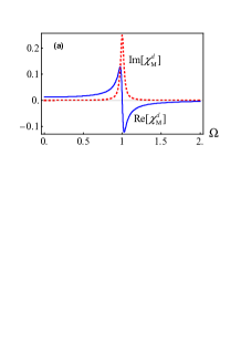
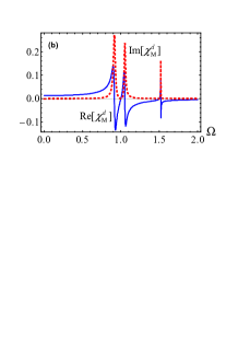
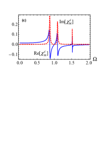
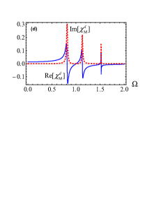
Figure 5: (Color online) The frequency dependence of the real part (the blue solid line) and the imaginary part (the red dashed line) of the magnetic susceptibility $\chi_{M}\left(\Omega\right)$. The values of $G_{1}$ and $G_{2}$ are: (a)$G_{1}=G_{2}=0$; (b)$G_{1}=0.03$ and $G_{2}=0.05$; (c)$G_{1}=G_{2}=0.05$; (d)$G_{1}=0.07$ and $G_{2}=0.05$. When $G_{1}$ and $G_{2}$ are not zero, the double-EIT effect appears with two absorption windows.

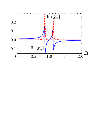
Figure 6: (Color online) The frequency dependence of the real part (the blue solid line) and the imaginary part (the red dashed line) of the magnetic susceptibility $\chi_{M}^{d}\left(\Omega\right)$ in some special situation, where the two absorption windows are reduced to one.

Finally, to witness the existence of the double-EIT phenomenon in our setup, we consider the velocity of signal transfer as follows. The group velocity of the alternating magnetic field propagating in the spin ensemble is defined as liyong1

$$v_{g} = \text{Re}\left[\frac{\mathrm{d}\Omega}{\mathrm{d}\left[\Omega n\left(\Omega\right)/c\right]}\right]$$ (39)

$$= \text{Re}\left[\frac{c}{n\left(\Omega\right)+\Omega\partial_{\Omega}n\left(\Omega\right)}\right],$$ (40)

where $n\left(\Omega\right)$ is the complex refractive index defined as

$$n\left(\Omega\right)=\sqrt{1+\chi_{M}\left(\Omega\right)},$$ (41)

and $c$ is the velocity of light in vacuum. The group velocity (in unit of the light velocity $c=1/\sqrt{\varepsilon_{0}\mu_{0}}$ in vacuum) in frequency region between the first and last two absorbed peaks, is illustrated in Fig. 7(a) and 7(b) respectively, with the parameters the same as that in Fig. 5(b). It is shown in Fig. 7 that in both of the two absorption windows, the group velocity of the microwave field is reduce dramatically. It is indeed similar to that in the atomic EIT effect.

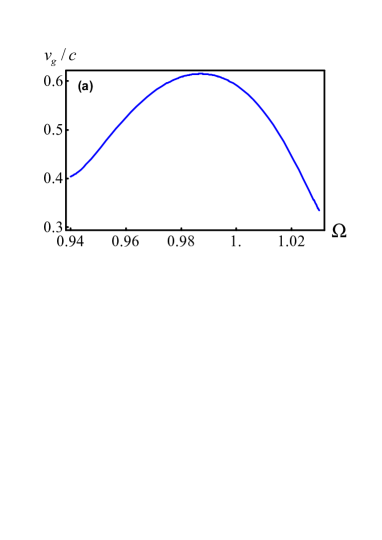
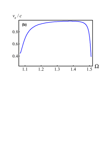
Figure 7: The group velocity $v_{g}$ in the frequency region between the first two [for (a)] and the last two [for (b)] absorbed peaks in Fig. 5(b). The microwave field’s group velocity is reduced dramatically in both of these two windows.

V Summary

We have proposed and studied a hybrid setup where two NAMRs are coupled to a nuclear spin ensemble to demonstrate quantum interference phenomenon, i.e., an analog of EIT in atomic ensemble coupled to light. This system is implemented by cantilevers tipped with ferromagnetic particles producing inhomogeneous magnetic fields which couple the mechanical tips to the spin ensemble. We have studied the dynamical properties in this NAMR-spin ensemble-NAMR system by applying a probe microwave field. In the low excitation approximation with large $N$ limit, this NAMR-spin ensemble-NAMR coupling system behaves as a system of three coupled harmonic oscillators. As a result, there is the so-called double-EIT effect in this system with two absorption windows. Furthermore, we have shown the group velocity of the microwave field is reduced dramatically in both of these two windows.

Finally, we point out that the NAMR-spin ensemble-NAMR coupling system is a sub-network of such a structure consisting of an array of NAMRs and nuclear spin ensembles, where the quantum information of the NAMR can be stored in the nuclear spin ensemble for long time and transferred to the next NAMR in a distance. And this process is repeated in the next sub-networks. Therefore, it is expected that the spin ensembles can behave as a quantum transducer that stores and transfer quantum information of the NAMRs.

- (1) D. Bouwmeeste, A. Ekert, and A. Zeilinger (Ed.), The Physics of Quantum Information (Springer, Berlin, 2000).
- (2) J. I. Cirac and P. Zoller, Phys. Rev. Lett. 74, 4091 (1995).
- (3) D. P. DiVincenzo and C. Bennet, Nature 404, 247 (2000).
- (4) Y. Li, T. Shi, B. Chen, Z. Song, and C. P. Sun, Phys. Rev. A 71, 022301 (2005).
- (5) T. Shi, Y. Li, Z. Song, and C. P. Sun, Phys. Rev. A 71, 032309 (2005).
- (6) S. E. Harris, Phys. Today 50 (7), 36 (1997).
- (7) L. V. Hau, S. E. Harris, Z. Dutton, and C. H. Behroozi, Nature 397, 594 (1999).
- (8) M. M. Kash, V. A. Sautenkov, A. S. Zibrov, L. Hollberg, G. R. Welch, M. D. Lukin, Y. Rostovtsev, E. S. Fry, and M. O. Scully, Phys. Rev. Lett. 82, 5229 (1999).
- (9) M. D. Lukin, M. Fleischhauer, A. S. Zibrov1, H. G. Robinson, V. L. Velichansky, L. Hollberg, and M. O. Scully, Phys. Rev. Lett. 79, 2959 (1997).
- (10) M. Fleischhauer and M. D. Lukin, Phys. Rev. Lett. 84, 5094 (2000).
- (11) D. F. Phillips, A. Fleischhauer, A. Mair, R. L. Walsworth, and M. D. Lukin, Phys. Rev. Lett. 86, 783 (2001).
- (12) C. Liu, Z. Dutton, C. H. Behroozi, L. V. Hau, Nature 409, 490 (2001).
- (13) C. P. Sun, Y. Li, and X. F. Liu, Phys. Rev. Lett. 91, 147903 (2003).
- (14) Y. Li and C. P. Sun, Phys. Rev. A 69, 051802(R) (2004).
- (15) Z. Song, P. Zhang, T. Shi, and C. P. Sun, Phys. Rev. B 71, 205314 (2005).
- (16) L. Zhou, Y. B. Gao, Z. Song, and C. P. Sun, Phys. Rev. A 77, 013831 (2008).
- (17) J. Q. Liao, J. F. Huang, Yu-xi Liu, L. M. Kuang, and C. P. Sun, Phys. Rev. A 80, 014301 (2009).
- (18) J. Q. Liao, Z. R. Gong, L. Zhou, Yu-xi Liu, C. P. Sun, and F. Nori, Phys. Rev. A 81, 042304 (2010).
- (19) J. M. Taylor, C. M. Marcus, and M. D. Lukin, Phys. Rev. Lett. 90, 206803 (2003).
- (20) M. H. Levitt, Spin Dynamics: Basics of Nuclear Magnetic Resonance, 2nd ed., (John Wiley & Sons, New York 2008)
- (21) A. Imamoḡlu, E. Knill, L. Tian, and P. Zoller, Phys. Rev. Lett. 91, 017402 (2003).
- (22) M. Poggio, G. M. Steeves, R. C. Myers, Y. Kato, A. C. Gossard, and D. D. Awschalom, Phys. Rev. Lett. 91, 207602 (2003).
- (23) M. Kroutvar, Y. Ducommun, D. Heiss, M. Bichler, D. Schuh, G. Abstreiter, and J. J. Finley, Nature 432, 81 (2004).
- (24) S. Mancini and P. Tombesi, Phys. Rev. A 49, 4055 (1994).
- (25) S. Bose, K. Jacobs, and P. L. Knight, Phys. Rev. A 59, 3204 (1999).
- (26) W. Marshall, C. Simon, R. Penrose, and D. Bouwmeester, Phys. Rev. Lett. 91, 130401 (2003).
- (27) D. Vitali, S. Gigan, A. Ferreira, H. R. Böhm, P. Tombesi, A. Guerreiro, V. Vedral, A. Zeilinger, and M. Aspelmeyer, Phys. Rev. Lett. 98, 030405 (2007).
- (28) C. Genes, D. Vitali, and P. Tombesi, Phys. Rev. A 77, 050307 (2008).
- (29) H. Ian, Z. R. Gong, Yu-xi Liu, C. P. Sun, and F. Nori, Phys. Rev. A 78, 013824 (2008).
- (30) Y. Chang, H. Ian, and C. P. Sun, J. Phys. B 42, 215502 (2009).
- (31) S. Mancini, D. Vitali, and P. Tombesi, Phys. Rev. Lett. 80, 688 (1998).
- (32) M. Bhattacharya and P. Meystre, Phys. Rev. Lett. 99, 073601 (2007).
- (33) M. Bhattacharya, H. Uys, and P. Meystre, Phys. Rev. A 77, 033819 (2008).
- (34) C. Genes, D. Vitali, P. Tombesi, S. Gigan, and M. Aspelmeyer, Phys. Rev. A 77, 033804 (2008).
- (35) K. Hammerer, K. Stannigel, C. Genes, and P. Zoller, P. Treutlein, S. Camerer, D. Hunger, and T. W. Hänsch, Phys. Rev. A 82, 021803(R) (2010).
- (36) S. Bose, K. Jacobs, and P. L. Knight, Phys. Rev. A 56, 4175 (1997).
- (37) Z. R. Gong, H. Ian, Yu-xi Liu, C. P. Sun, and F. Nori, Phys. Rev. A 80, 065801 (2009).
- (38) M. Wallquist, K. Hammerer, P. Zoller, C. Genes, M. Ludwig, F. Marquardt, P. Treutlein, J. Ye, H. J. Kimble, Phys. Rev. A 81, 023816 (2010).
- (39) K. C. Schwab and M. L. Roukes, Phys. Today 58, 36 (2005).
- (40) L. G. Remus, M. P. Blencowe, Y. Tanaka, Phys. Rev. B 80, 174103 (2009).
- (41) D. Rugar, C. S. Yannoni, J. A. Sidles, Nature 360, 563 (1992).
- (42) J. A. Sidles, J. L. Garbini, K. J. Bruland, D. Rugar, O. Züger, S. Hoen, and C. S. Yannoni, Rev. Mod. Phys. 67, 249 (1995).
- (43) D. Rugar, R. Budakian, H. J. Mamin, and B. W. Chui, Nature 430, 329 (2004).
- (44) R. Budakian, H. J. Mamin, B. W. Chui, D. Rugar, Science 307, 408 (2005).
- (45) H. J. Mamin, M. Poggio, C. L. Degen, D. Rugar, Nat. Nano. 2, 301 (2007).
- (46) C. L. Degen, M. Poggio, H. J. Mamin, and D. Rugar, Phys. Rev. Lett. 99, 250601 (2007).
- (47) C. L. Degen, M. Poggio, H. J. Mamin, and D. Rugar, Phys. Rev. Lett. 100, 137601 (2008).
- (48) Fei Xue, Ling Zhong, Yong Li, and C. P. Sun, Phys. Rev. B 75, 033407 (2007).
- (49) M. Poggio, H. J. Mamin, C. L. Degen, M. H. Sherwood, and D. Rugar, Phys. Rev. Lett. 102, 087604 (2009).
- (50) P. C. Layterbur, Nature 242, 190 (1973).
- (51) P. Rabl, S. J. Kolkowitz, F. H. L. Koppens, J. G. E. Harris, P. Zoller, M. D. Lukin, Nat. Phys. 6, 602 (2010).
- (52) C. P. Sun, L. F. Wei, Yu-xi Liu, and F. Nori, Phys. Rev. A 73, 022318 (2006).
- (53) M. O. Scully and M. S. Zubairy, Quantum Optics (Cambridge University Press, Cambridge, 1997).
- (54) C. L. G. Alzar, M. A. G. Martinez, and P. Nussenzveig, Am. J. Phys. 70, 37 (2002).
- (55) J. D. Jackson, Classical Electrodynamics, 3rd ed. (John Wiley & Sons, New York, 1999).
- (56) M. N. Makhonin, E. A. Chekhovich, P. Senellart, A. Lemaître, M. S. Skolnick, and A. I. Tartakovskii, Phys. Rev. B 82, 161309(R) (2010).