Extended Quantum Dimer Model and novel valence-bond phases

Abstract

We extend the quantum dimer model (QDM) introduced by Rokhsar and Kivelson so as to construct a concrete example of the model which exhibits the first-order phase transition between different valence-bond solids suggested recently by Batista and Trugman and look for the possibility of other exotic dimer states. We show that our model contains three exotic valence-bond phases (herringbone, checkerboard and dimer smectic) in the ground-state phase diagram and that it realizes the phase transition from the staggered valence-bond solid to the herringbone one. The checkerboard phase has four-fold rotational symmetry, while the dimer smectic, in the absence of quantum fluctuations, has massive degeneracy originating from partial ordering only in one of the two spatial directions. A resonance process involving three dimers resolves this massive degeneracy and dimer smectic gets ordered (order from disorder).

Quantum Dimer Model,Valence-Bond Solid,:

1 Introduction

Since P.W. Anderson’s paper[1, 2, 3] in 1973, the quest for the resonating valence bond (RVB) state[4, 5, 6, 7] and exotic valence bond solids (VBS)[8, 9, 10, 11, 12] have been one of the recurrent themes in research on frustrated antiferro(AF) magnets[13, 14, 15]. One of the most studied problem of frustrated magnets would be the ground-state property of the $J_{1}$-$J_{2}$ Heisenberg model on a square lattice[16, 17, 18, 19] especially around the fully frustrated point $J_{2}/J_{1}=1/2$. Chandra and Doucot[16], on the basis of a 1/S expansion for the sublattice magnetization, have predicted that the Néel order vanishes for $J_{2}/J_{1}$ $\simeq$ 0.38 and suggested that for a range of $J_{2}/J_{1}$ beyond 0.38 the ground state might be a spin liquid. Nishimori and Saika[20] used the modified spin wave approximation to conclude that a first-order phase transition from the Néel phase to the collinear AF phase[21] occurs. Gelfand, Singh and Huse[10] have argued that system gets spontaneously dimerized in the columnar pattern as has been predicted by Read and Sachdev[22]. In spite of these intensive studies, nature of the ground state of the square-lattice $J_{1}$-$J_{2}$ Heisenberg model around the fully frustrated point $J_{2}/J_{1}=1/2$ is still controversial.

One natural way to optimize the (short-range) antiferromagnetic correlation in quantum (i.e. low-spin) magnets is pairing spins at short distance into spin-singlet dimers. Therefore, it is tempting to consider the quantum dynamics within the spin-singlet subspace made up of all possible (short-range) dimer coverings. Quantum dimer model (QDM), which has been originally introduced by Rokhsar and Kivelson[23] to describe the low-energy physics of the square-lattice Heisenberg antiferromagnet, is now considered to capture a certain aspect of the low-energy dynamics of (frustrated) non-magnetic Mott insulators. The standard QDMs á la Rokhsar and Kivelson are defined in the Hilbert space of the nearest-neighbor dimer coverings of the lattice and consists only of processes which involve a single dimer pair. The square-lattice QDM thus defined is known to exhibit crystalline orders of the valence bonds and confined spinons except at the Rokhsar-Kivelson (RK) point[23], where a short ranged RVB state is realized (see Refs. [24, 25] for readable reviews of QDM).

Of course, the Rokhsar-Kivelson QDM is a minimal model that describes the dynamics of singlet dimers; for instance, when one derives QDM from a given microscopic model by the overlap expansion, various higher-order terms (including dimer moves on larger loops) are generated. Along this line, Ralko et al.[26, 27] has considered an extension of the QDM and investigated the impact of higher-order processes included. Among other attempts at extending QDM, Papanikolaou et al.[28] have introduced, on the basis of an analogy to the Pokrovsky-Talapov model[29] of fluctuating domain walls in two-dimensional classical statistical mechanics[30, 31, 32, 33], a two-dimensional microscopic model of interacting quantum dimers, which, in principle, involves infinitely many arbitrary parameters and dimer patterns.

Recently, Batista and Trugman[34] have undertaken a different microscopic approach and considered an $S=1/2$ $J_{1}$-$J_{2}$ Heisenberg model with an additional term (four-spin exchange interactions) that makes the model quasi-exactly solvable at the fully frustrated point $J_{2}/J_{1}=1/2$ (see Ref. [8] for a similar approach in spirit). They have argued that any states having at least one singlet dimer per plaquette are ground states. Although one can easily see that the staggered- and the herringbone VBS[28] (dubbed ‘zigzag dimer’ in Ref.[34]) are possible candidates of the ground states of their Hamiltonian, it is not clear when one of these VBSs becomes the unique ground state or what interaction controls the phase transition between them and it is known that the simplest QDM does not exhibit such a first-order transition[35, 36, 37]. Motivated by this question, we shall extend QDM so as to realize the first-order phase transition suggested in Ref.[34] and seek for other exotic dimer states and then map out (a part of) the phase diagram. This is the main purpose of this paper.

This paper is structured as follows. In section 2, we study a certain region of EQDM in the absence of quantum fluctuations and, as the result, find a new disordered phase dubbed dimer smectic. The main motivation comes from a first-order transition between the staggered VBS and the herringbone VBS which has been predicted recently by Batista and Trugman[34] to be controlled by a certain unspecified parameter ‘g’. We show that by changing one of the coupling constants in our EQDM we can indeed drive the first-order transition. Within the usual QDM, both VBSs (staggered and herringbone) are exactly degenerate zero-energy states of the (classical) Hamiltonian and the single-plaquette resonance does not lift the degeneracy. In section 3, we consider the effects of quantum fluctuations. Specifically, we calculate the quantum correction to the ground-state energy for the three valence-bond states (herringbone, checkerboard VBSs and dimer smectic) which are degenerate in the absence of fluctuations (resonances) and see whether the degeneracy is resolved or not. We show that dimer smectic eventually gets ordered by a new resonance term which is equivalent to two successive actions of the familiar parallel dimer resonance. In A, we discuss an interesting mapping between the EQDM and a spin-1 model which is helpful in writing down the EQDM Hamiltonian in terms of a relatively small number of coupling constants. In B, we present the second-order calculation of the energy shift (eq.8) caused by the $t^{\prime}$ resonance effect for the dimer smectic.

2 Extended Quantum Dimer Model

Recently, Batista and Trugman[34] have introduced the following generalized $S=1/2$ $J_{1}$-$J_{2}$ Heisenberg model on a square lattice including an additional term (a four-spin exchange interaction) that makes a quasi-exact solution feasible at the fully frustrated point $J_{2}/J_{1}=1/2$:

$${\cal H}_{\rm{BT}} ={\cal{H}}_{J_{1}\rm{-}J_{2}}+{\cal{H}}_{\rm{exchange}}$$ (1)

$$=J_{1}\sum_{\langle i,j\rangle}\vec{S}_{i}\cdot\vec{S}_{j}+\frac{J_{1}}{2}\sum_{\langle\!\langle i,j\rangle\!\rangle}\vec{S}_{i}\cdot\vec{S}_{j}+\frac{J_{1}}{8}\sum_{\alpha}\left(P^{\alpha}_{ij}P^{\alpha}_{kl}+P^{\alpha}_{jk}P^{\alpha}_{il}+P^{\alpha}_{ik}P^{\alpha}_{jl}\right)$$

$$=\frac{3J_{1}}{2}\sum_{\alpha}\cal{P}^{\alpha}\;,$$

where $\langle i,j\rangle$ and $\langle\!\langle i,j\rangle\!\rangle$ denote the nearest neighbors and the second nearest neighbors, respectively, and $P_{ij}=S_{i}\cdot S_{j}$. The index $\alpha$ labels the plaquettes and ijkl are the four sites of each plaquette in the clockwise order. The four-spin exchange interaction ${\cal{H}}_{\rm{exchange}}$ is similar to the usual four-spin cyclic exchange[38] except that the sign of the last term is different. Since the operator $\cal{P}^{\alpha}$ projects the spin state of the plaquette $\alpha$ onto the subspace with total spin $S^{\alpha}_{T}=2$, it is clear[34] that any states having at least one singlet dimer on each plaquette can be the ground states. Of course, there are many other configurations[34] where we have dimers on diagonal bonds or unpaired $S=1/2s$. Nevertheless, we will not consider these configurations hereafter.

Though both the staggered- and the herringbone VBS (which is called ‘zigzag dimer’ in Ref.[34]) satisfy the condition for the ground states described above, it is not clear when and how one of these VBSs is chosen as the unique ground state. Also the control parameter that drives the first-order transition from the staggered dimer to herringbone predicted in Ref. [34] has not been identified yet either.

Motivated by these, we generalize the usual QDM and consider the following extended quantum dimer model (EQDM):

$${\cal H}_{\rm{EQDM}}=\sum_{\Box}\Biggl{\{} -t\,\bigl{|}\,\raisebox{-4.30554pt}{\includegraphics[scale={0.3}]{VB1.eps}}\,\bigr{\rangle}\bigl{\langle}\,\raisebox{-4.30554pt}{\includegraphics[scale={0.3}]{VB2.eps}}\,\bigr{|}-t^{\prime}\,\Bigl{|}\,\raisebox{-8.61108pt}{\includegraphics[scale={0.3}]{VB3.eps}}\,\Bigr{\rangle}\Bigl{\langle}\,\raisebox{-8.61108pt}{\includegraphics[scale={0.3}]{VB4.eps}}\,\Bigr{|}-t^{\prime\prime}\,\Bigl{|}\,\raisebox{-12.91663pt}{\includegraphics[scale={0.3}]{VB7.eps}}\,\Bigr{\rangle}\Bigl{\langle}\,\raisebox{-12.91663pt}{\includegraphics[scale={0.3}]{VB9.eps}}\,\Bigr{|}$$ (2)

$$+(-4J+2J^{\prime}+\lambda)\,\bigl{|}\,\raisebox{-4.30554pt}{\includegraphics[scale={0.3}]{VB2.eps}}\,\bigr{\rangle}\bigl{\langle}\,\raisebox{-4.30554pt}{\includegraphics[scale={0.3}]{VB2.eps}}\,\bigr{|}-J\,\Bigl{|}\,\raisebox{-8.61108pt}{\includegraphics[scale={0.3}]{VB5.eps}}\,\Bigr{\rangle}\Bigl{\langle}\,\raisebox{-8.61108pt}{\includegraphics[scale={0.3}]{VB5.eps}}\,\Bigr{|}$$

$$-J^{\prime}\,\Bigl{|}\,\raisebox{-8.61108pt}{\includegraphics[scale={0.3}]{VB3.eps}}\,\Bigr{\rangle}\Bigl{\langle}\,\raisebox{-8.61108pt}{\includegraphics[scale={0.3}]{VB3.eps}}\,\Bigr{|}+(-2J+J^{\prime}+\kappa)\,\Bigl{|}\,\raisebox{-4.30554pt}{\includegraphics[scale={0.3}]{VB8.eps}}\,\Bigr{\rangle}\Bigl{\langle}\,\raisebox{-4.30554pt}{\includegraphics[scale={0.3}]{VB8.eps}}\,\Bigr{|}$$

$$+J^{\prime}\,\Bigl{|}\,\raisebox{-12.91663pt}{\includegraphics[scale={0.3}]{VB7.eps}}\,\Bigr{\rangle}\Bigl{\langle}\,\raisebox{-12.91663pt}{\includegraphics[scale={0.3}]{VB7.eps}}\,\Bigr{|}+(\rm{h.c.})+(\rm{rotations})+(\rm{reflections})\Biggr{\}}.\$$

Except for the last term (with the coefficient $J^{\prime}$), the above EQDM contains all possible dimer patterns having at least one singlet dimer on each plaquette (with the coefficients given by $-J$, $-J^{\prime}$, and $(-2J+J^{\prime}+\kappa)$); the last one appears in the process of deriving the EQDM from the pseudo-spin ($S=1$) Hamiltonian described in the Appendix. However, if we choose the coupling constants as in (A.12)-(A.15), this configuration becomes higher in energy and we may expect that the EQDM hopefully becomes an effective Hamiltonian for the generalized $S=1/2$ $J_{1}$-$J_{2}$ Heisenberg model of Batista and Trugman[34].

We will study the region $J^{\prime}=2J(>0)$, $0\leq\lambda<2J$ and $\kappa<0$ where the two valence-bond states – the staggered dimer and the herringbone– compete with each other in the ground state and see that the three-spin interaction $`\kappa^{\prime}$ in the pseudo-spin Hamiltonian (see Appendix for the definition) plays a role of the unspecified control parameter $`g^{\prime}$ in Ref. [34]. On the $\lambda=0$ line, a more exotic phase dubbed dimer smectic will be found.

2.1 Phase diagram in $J^{\prime}=2J(>0)$, $0\leq\lambda<2J$ and $\kappa<0$

In this region ($J^{\prime}=2J$ ($>$0)), the EQDM is rewritten as

$${\cal H}_{\rm{EQDM}} =\sum_{\Box}\Biggl{\{}-t\,\bigl{|}\,\raisebox{-4.30554pt}{\includegraphics[scale={0.3}]{VB1.eps}}\,\bigr{\rangle}\bigl{\langle}\,\raisebox{-4.30554pt}{\includegraphics[scale={0.3}]{VB2.eps}}\,\bigr{|}-t^{\prime}\,\Bigl{|}\,\raisebox{-8.61108pt}{\includegraphics[scale={0.3}]{VB3.eps}}\,\Bigr{\rangle}\Bigl{\langle}\,\raisebox{-8.61108pt}{\includegraphics[scale={0.3}]{VB4.eps}}\,\Bigr{|}-t^{\prime\prime}\,\Bigl{|}\,\raisebox{-12.91663pt}{\includegraphics[scale={0.3}]{VB7.eps}}\,\Bigr{\rangle}\Bigl{\langle}\,\raisebox{-12.91663pt}{\includegraphics[scale={0.3}]{VB9.eps}}\,\Bigr{|}$$ (3)

$$\ \ \ \ \ \ \ \ \ \ \ \ \ +\lambda\,\bigl{|}\,\raisebox{-4.30554pt}{\includegraphics[scale={0.3}]{VB2.eps}}\,\bigr{\rangle}\bigl{\langle}\,\raisebox{-4.30554pt}{\includegraphics[scale={0.3}]{VB2.eps}}\,\bigr{|}-J\,\Bigl{|}\,\raisebox{-8.61108pt}{\includegraphics[scale={0.3}]{VB5.eps}}\,\Bigr{\rangle}\Bigl{\langle}\,\raisebox{-8.61108pt}{\includegraphics[scale={0.3}]{VB5.eps}}\,\Bigr{|}-2J\,\Bigl{|}\,\raisebox{-8.61108pt}{\includegraphics[scale={0.3}]{VB3.eps}}\,\Bigr{\rangle}\Bigl{\langle}\,\raisebox{-8.61108pt}{\includegraphics[scale={0.3}]{VB3.eps}}\,\Bigr{|}$$

$$\ \ \ \ \ \ \ \ \ \ \ \ \ +\kappa\,\Bigl{|}\,\raisebox{-4.30554pt}{\includegraphics[scale={0.3}]{VB8.eps}}\,\Bigr{\rangle}\Bigl{\langle}\,\raisebox{-4.30554pt}{\includegraphics[scale={0.3}]{VB8.eps}}\,\Bigr{|}+2J\,\Bigl{|}\,\raisebox{-12.91663pt}{\includegraphics[scale={0.3}]{VB7.eps}}\,\Bigr{\rangle}\Bigl{\langle}\,\raisebox{-12.91663pt}{\includegraphics[scale={0.3}]{VB7.eps}}\,\Bigr{|}$$

$$\ \ \ \ \ \ \ \ \ \ \ \ \ +(\rm{h.c.})+(\rm{rotations})+(\rm{turnover})\Biggr{\}}.$$

We restrict our investigation to the region $\lambda\geq 0$ because otherwise the staggered dimer and the herringbone are not competing, and such situation is not relevant to our current purpose.

In the first step, we consider the case where quantum fluctuations (i.e. the resonances $t$, $t^{\prime}$ and $t^{\prime\prime}$) are absent. The phase diagram for $t=t^{\prime}=t^{\prime\prime}=0$ is given in Fig.1. (A) $0<\lambda<2J$; it is clear that the phase transition from the staggered-VBS to the herringbone-VBS occurs by changing the parameter $\kappa$, which is the coefficient of three-spin interaction in the pseudo-spin Hamiltonian given in Appendix. The critical value is $\kappa_{\rm{c}}=-J$. Namely, the three-spin interaction ‘$\kappa$’ in the pseudo-spin Hamiltonian plays a role of the unspecified control parameter ‘$g$’ in Ref.[34]. In this sense, EQDM may be an effective Hamiltonian for a $J_{1}$-$J_{2}$ Heisenberg model with a four-spin interaction introduced by Batista and Trugman in this region. It is worth mentioning that the usual QDM cannot describe the transition from staggered to herringbone VBS, since both are exactly degenerate zero-energy eigenstates of the QDM Hamiltonian regardless of the parameters. (B) $\lambda=0$; Two novel kinds of VBS, the checkerboard VBS (Fig.2) and the dimer smectic (Fig.2), emerge and are degenerate with the herringbone-VBS ($\kappa\geq-J$). In the next section, we will discuss how to resolve this degeneracy by the effects of resonance ($t,t^{\prime}$,$t^{\prime\prime}$) in detail.

On the $\kappa=-J$ and $\lambda=0$ point the ground state is highly degenerate and Z₄-vortex (Fig.5) emerges.

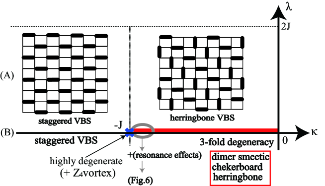
Figure 1: (Color online) Phase diagram of EQDM for $t=t^{\prime}=t^{\prime\prime}=0$, $0\leq\lambda<2J$. Basically $\kappa$ controls the phase transition from staggered-VBS to herringbone-VBS. On $\lambda=0,\kappa>-J$ line checkerboard-VBS and dimer smectic emerge and are degenerate with herringbone-VBS.

2.2 The Features of VBS Phases

Now let us discuss the main features of these VBSs.

(i) Herringbone; The hallmark of this state is that it contains no parallel dimer. In fact, the herringbone shares this important property with the well-known staggered VBS[23]; there is no flippable (with respect to $t$, $t^{\prime}$ and $t^{\prime\prime}$) dimers in both VBSs. In this sense, both the herringbone and the staggered VBS are total free from the resonance and robust.

(ii) Checkerboard VBS[39]; this VBS is made up of a checkerboard pattern of two kinds of parallel dimers and has the four-fold rotational symmetry .

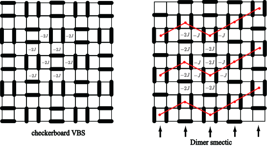
Figure 2: (Color online) [Left] Checkerboard. This VBS is characterized by a checkerboard pattern of parallel dimers and has the four-fold rotational symmetry. [Right] Dimer smectic. This is realized by arranging (b) plaquettes in Fig.10 in such a way that the number of (b) plaquettes is maximal within each column and then connecting these ‘ordered’ columns horizontally by the herringbone-like (d) plaquettes in Fig.10.

(iii) Dimer smectic; this VBS corresponds in a sense to the intermediate between the checkerboard and the herringbone, which means that this is realized by arranging (b) plaquettes in Fig.10 in such a way that the number of (b) plaquettes is maximal within each column and then connecting these ‘ordered’ columns horizontally by the herringbone-like (d) plaquettes in Fig.10. The horizontal order is formed so as to break the translation symmetry. In other words, there are two ways (type-($\eta$) and ($\tau$) in Fig.3) of forming the herringbone-like order horizontally. If the integers $N_{x}$ and $N_{y}$ are the linear dimensions of the lattice (the lattice spacing is set to unity) and we set $N_{\eta}$ and $N_{\tau}$ the numbers of the stripes of type-($\eta$) and ($\tau$), they must satisfy

$$2N_{\eta}+2N_{\tau}=N_{x}.$$ (4)

From this, one sees that the horizontal herringbone-like order type-($\eta$ ) and ($\tau$) not only break the translation symmetry but also lead to extensive GS degeneracy since any combinations of ($\textit{N}_{\eta},\textit{N}_{\tau}$) are permitted if they only satisfy eq.(4). This huge degeneracy comes from the fact that pure (local) energetics cannot determine the ground state uniquely and is reminiscent of similar degeneracy in such geometrically frustrated magnets as the Kagomé antiferromagnet[40] and the pyrochlore antiferromagnet[41].

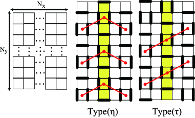
Figure 3: (Color online) Two possible configurations of three neighboring columns in dimer smectic. These two patterns are the building blocks in forming highly degenerate order in the horizontal direction.

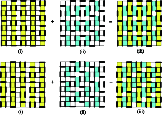
Figure 4: (Color online) Plaquette tiling of stripe. Hatched columns in panel-(i) may be viewed as one-dimensional solids consisting of type-(b) plaquettes and these columns are connected to each other by ‘binding energy’ provided by the interaction energy of herringbone-like (hatched) plaquettes in panel-(ii).

(iv) Z₄-vortex; this VBS becomes one of the ground states only at the special point $\lambda=0,\kappa=-J$ (shown in Fig.1 as ‘highly degenerate’). This phase consists of four domains each of which assumes one of the four possible staggered VBS patterns (see Fig.5). We call this phase $\mathbb{Z}_{4}$-vortex because the following order parameter ${\cal O}_{\mathbb{Z}_{4}}$ in fact changes its value like a $\mathbb{Z}_{4}$-variable ($1\rightarrow i\rightarrow-1\rightarrow-i$) as we move around the origin (see Fig.5):

$${\cal O}_{\mathbb{Z}_{4}}\equiv \frac{1}{N_{\rm{site}}}\sum_{\vec{r}}(-1)^{\vec{r}_{x}+\vec{r}_{y}}\Bigl{\{}(\vec{S}_{\vec{r}}\cdot\vec{S}_{\vec{r}+\vec{e}_{x}}-\vec{S}_{\vec{r}+\vec{e}_{y}}\cdot\vec{S}_{\vec{r}+\vec{e}_{x}+\vec{e}_{y}})$$ (5)

$$\ \ \ \ \ \ \ \ \ \ \ \ \ \ \ \ \ \ \ \ \ \ \ \ \ \ +i(\vec{S}_{\vec{r}}\cdot\vec{S}_{\vec{r}+\vec{e}_{y}}-\vec{S}_{\vec{r}+\vec{e}_{x}}\cdot\vec{S}_{\vec{r}+\vec{e}_{x}+\vec{e}_{y}})\Bigr{\}}\;.$$

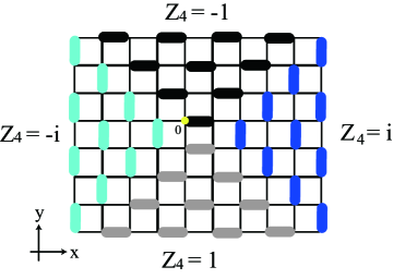
Figure 5: (Color online) Illustration of the $Z_{4}$ vortex. Four dimer domains are characterized by four different values ($1,-1,i,-i$) of order parameter ${\cal O}_{\mathbb{Z}_{4}}$.

3 Effects of Quantum Fluctuations

3.1 Energy corrections from resonance terms

In this section, we investigate how the degeneracy among the three valence-bond phases (herringbone, checkerboard and dimer smectic) found in the previous section is resolved for $J^{\prime}=2J(>0),\lambda=0$ and $\kappa=-(J+h)$ (circled region in Fig.1) paying particular attention to the fate of the huge ground-state degeneracy in the dimer smectic. First let us recover the resonance terms $t$, $t^{\prime}$ and $t^{\prime\prime}$ as perturbation to the diagonal part:

$$V_{\rm{perturb}} =\sum_{\Box}\left\{-t\,\bigl{|}\,\raisebox{-4.30554pt}{\includegraphics[scale={0.3}]{VB1.eps}}\,\bigr{\rangle}\bigl{\langle}\,\raisebox{-4.30554pt}{\includegraphics[scale={0.3}]{VB2.eps}}\,\bigr{|}-t^{\prime}\,\Bigl{|}\,\raisebox{-8.61108pt}{\includegraphics[scale={0.3}]{VB3.eps}}\,\Bigr{\rangle}\Bigl{\langle}\,\raisebox{-8.61108pt}{\includegraphics[scale={0.3}]{VB4.eps}}\,\Bigr{|}-t^{\prime\prime}\,\Bigl{|}\,\raisebox{-12.91663pt}{\includegraphics[scale={0.3}]{VB7.eps}}\,\Bigr{\rangle}\Bigl{\langle}\,\raisebox{-12.91663pt}{\includegraphics[scale={0.3}]{VB9.eps}}\,\Bigr{|}\right\}$$ (6)

$$\ \ \ \ \ \ \ \ \ \ \ +(\rm{rotations})+(\rm{h.c.}).$$

The resonance terms $t$, $t^{\prime}$ and $t^{\prime\prime}$ are assumed to be very small (i.e. $0<t,t^{\prime},t^{\prime\prime}\ll J$), and will be used as the small parameters in perturbation theory. These perturbing terms come into play for the first time at the second order and we have to consider the effects of resonance terms up to this order.

$$E_{\rm{resonance}}^{\rm{check}} =-JN_{x}N_{y}-\frac{t^{\prime 2}}{4J}\frac{N_{x}N_{y}}{2}-\frac{t^{2}}{12J}\frac{N_{x}N_{y}}{4}-\frac{t^{\prime\prime 2}}{6J}\frac{N_{x}N_{y}}{4}.$$ (7)

$$E_{\rm{resonance}}^{\rm{smectic}} =-JN_{x}N_{y}-\frac{t^{\prime 2}}{4J-2h}N_{\eta}\frac{N_{y}}{3}-\frac{t^{\prime 2}}{10J}N_{\eta}\frac{N_{y}}{3}-\frac{t^{\prime 2}}{7J-h}N_{\tau}\frac{2N_{y}}{3}$$ (8)

$$\ \ \ \ \ -\frac{t^{2}}{4J}\frac{N_{x}}{2}\frac{N_{y}}{3}-\frac{t^{\prime\prime 2}}{16J-2h}\frac{N_{x}N_{y}}{6}.$$

$$E_{\rm{resonance}}^{\rm{herring}} =-JN_{x}N_{y}.\$$ (9)

The pair of integers $(N_{\eta},N_{\tau})$ has been defined in section 3 and satisfies

$$2N_{\eta}+2N_{\tau}=N_{x}\;.$$ (10)

We now rescale the couplings as $\tilde{t}\equiv t/J$ and $\tilde{h}\equiv h/J$ and define $\bar{N_{\eta}}\equiv N_{\eta}/N_{x}$ so that $\bar{N_{\eta}}$ must satisfy $0\leq\bar{N_{\eta}}\leq 1/2$. The parameter $|h|$ is assumed to be very small ($|h|\ll J$) and we approximate $\tilde{h}^{2}\sim 0$. Then, the scaled energy $\widetilde{E}_{\rm{resonance}}^{\rm{smectic}}\equiv E_{\rm{resonance}}^{\rm{smectic}}/J$ is given by

$$\frac{\widetilde{E}_{\rm{resonance}}^{\rm{smectic}}}{N_{x}N_{y}}\simeq-1-\frac{\tilde{t}^{2}}{24}-\frac{\tilde{t}^{\prime 2}}{21}\left(1+\frac{\tilde{h}}{7}\right)-\frac{\tilde{t}^{\prime 2}}{140}\bar{N}_{\eta}\left(3+\frac{55}{14}\tilde{h}\right)-\frac{\tilde{t}^{\prime\prime 2}}{96}\left(1+\frac{\tilde{h}}{8}\right).$$ (11)

It is apparent that only the resonance $\tilde{t}^{\prime}$ depends on the number of stripe type (($\eta$) and ($\tau$)) in dimer smectic (fourth term in the right hand side). Since $|h|$ is so small, we may safely assume that the coefficient of $\bar{N}_{\eta}$ is negative. Then, one can easily see that quantum fluctuations ($t^{\prime}$) form a minimum of the energy of the dimer smectic at $\bar{N}_{\eta}=1/2$ thereby select one particular configuration, which is shown in the lower panel of Fig.7, as the ground state. This is because when $|h|$ is small enough, type($\eta$) configuration can gain more resonance ($t^{\prime}$) energy than the type($\tau$) one and the total energy is minimized when all the columns are of the type($\eta$).

Thus resonance $\tilde{t}^{\prime}$ which is equivalent to two successive actions of the usual parallel dimer resonance ($\tilde{t}$) and ignored in the standard QDM plays a special role; it resolves the high degeneracy through the order-by-disorder mechanism[43, 44].

Then the energy of ordered dimer smectic is evaluated as

$$\frac{\widetilde{E}_{\rm{resonance}}^{\rm{smectic}}}{N_{x}N_{y}}\simeq-1-\frac{\tilde{t}^{2}}{24}-\frac{\tilde{t}^{\prime 2}}{120}\alpha-\frac{\tilde{t}^{\prime\prime 2}}{96}\left(1+\frac{\tilde{h}}{8}\right).$$ (12)

$$\alpha\equiv 7+\frac{5}{2}\tilde{h}\;.$$ (13)

By comparing the energies of the three phases, we can draw the phase diagram of EQDM in this region (Fig.6).

$$\widetilde{E}_{\rm{resonance}}^{\rm{smectic}}<\widetilde{E}_{\rm{resonance}}^{\rm{check}} \Longleftrightarrow\tilde{t}^{2}>6\left(1-\frac{\alpha}{15}\right)\tilde{t}^{\prime 2}+\left(\frac{3}{2}-\frac{\tilde{h}}{16}\right)\tilde{t}^{\prime\prime 2}.$$ (14)

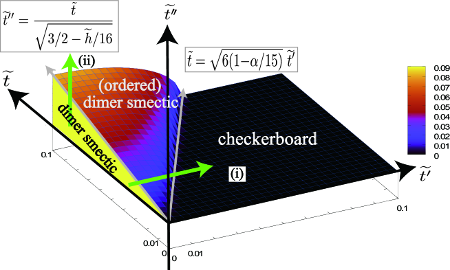
Figure 6: (Color online) Schematic phase diagram of EQDM with $t$-$t^{\prime}$-$t^{\prime\prime}$axis for $J^{\prime}=2J(>0),\lambda=0,\kappa=-(J+h)$. Parameter $h$ takes small negative values. Highly degenerate dimer smectic exists only within a region on the $\tilde{t^{\prime}}=0$ plane specified by $\tilde{t}^{\prime\prime}<\tilde{t}(\frac{3}{2}-\frac{\tilde{h}}{16})^{-1/2}$. In the region shown as ‘(ordered) dimer smectic’, a unique ground state is selected by the resonance $\tilde{t}^{\prime}$. Boundary between ordered dimer smectic and checkerboard VBS is given by eq.(33).

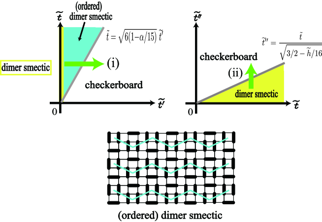
Figure 7: (Color online) Schematic phase diagram of EQDM with ($\tilde{t}^{\prime}$-$\tilde{t}$) plane and ($\tilde{t}$-$\tilde{t}^{\prime\prime}$)plane for $J^{\prime}=2J(>0),\lambda=0,\kappa=-(J+h)$. Parameter $h$ is a small negative value. Dimer smectic gets ordered only by resonance $\tilde{t}^{\prime}$ (see arrow (i)). Because the phases on either side of the boundary have totally different symmetries, we may expect that the transition is of first order.

As shown in Fig.7 dimer smectic gets ordered by resonance $t^{\prime}$ on ($\tilde{t}^{\prime}$-$\tilde{t}$) plane and resonance $\tilde{t}^{\prime}$ drives the phase transition from dimer smectic to checkerboard VBS through ordered dimer smectic. On the other hand, on ($\tilde{t}$-$\tilde{t}^{\prime\prime}$) plane (without $t^{\prime}$ resonance) because there is no resonance $t^{\prime}$ effects that dimer smectic does not get ordered and the phase transition from dimer smectic to checkerboard VBS occurs without ordered dimer smectic phase.

Because the phases on either side of the boundary have totally different symmetries, we may expect that the transition is of first order.

3.2 Finite temperatures

It would be interesting to consider how the above one-dimensional solids in dimer smectic phase melt into disordered states at finite temperatures. In fact, this kind of columnar structures reminds us of the smectic metal state in strongly-correlated systems[45, 46] and the sliding phases in liquid crystals[47] or in frustrated spin systems[48, 49]. Below, we give a brief discussion about the possibility of the sliding behavior in the dimer smectic phase.

The energy cost necessary to slide a column (a one-dimensional solid) vertically and destroy the dimer-smectic (i.e. herringbone-like) order is estimated as (see Fig.8)

$$\Delta E_{\rm{shift}}^{\rm{smectic}}\sim O(N_{y})\;.$$ (15)

On the other hand, the energy to destroy a one-dimensional solid itself is estimated as

$$\Delta E_{\rm{column}}^{\rm{smectic}}\sim O(1),$$ (16)

because we can adjust dimer configurations so as to minimize the effects of breakdown in one-dimensional solid (see Fig.8). These values suggest that as the temperature is increased, one-dimensional solids themselves are destroyed in the first place and exclude the possibility of the phase of fluctuating one-dimensional solids.

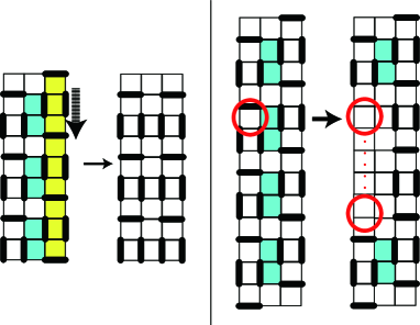
Figure 8: (Color online) [Left] Shift of a solid column (the rightmost one) in the vertical direction destroys the herringbone-like order (hatched plaquettes in the middle column). The necessary energy cost is estimated as $\Delta E_{\rm{shift}}^{\rm{smectic}}\sim O(N_{y})$. [Right] Destruction of a columnar (1D) solid itself occurs by the insertion of wrong plaquettes into the column. The energy to destroy one-dimensional solid itself is estimated as $\Delta E_{\rm{column}}^{\rm{smectic}}\sim O(1)$.

4 Summary

In the usual QDM of Rokhsar and Kivelson , the staggered- and the herringbone VBS should be degenerate, because both VBSs are zero-energy states and have no plaquettes on which resonance term ($t$) and diagonal term (pair dimer) can act.

In the present paper, we have extended QDM so as to describe the phase transition from the staggered VBS to the herringbone VBS. We can include all (nearest-neighbor) dimer configurations which have at least one dimer in each plaquette. Therefore, EQDM is considered in a sense to be a generalization of $S=1/2$ the $J_{1}$-$J_{2}$ model with four-spin exchange interactions[34] at its fully frustrated point ($J_{1}=2J_{2}$).

We then mapped out the phase diagram of EQDM in the region where both the staggered VBS and the herringbone VBS exist as the ground states ($J^{\prime}=2J(>0),\lambda=0,\kappa=-(J+h)$) by the second-order perturbation theory in quantum fluctuations $t$, $t^{\prime}$ and $t^{\prime\prime}$. We have found that the three-spin interaction $`\kappa^{\prime}$ in the pseudo-spin Hamiltonian plays a role of the unspecified control parameter ‘g’ suggested by Batista and Trugman which drives the first-order phase transition between the above two VBS phases. We have also found that there does exist a new VBS phase called the dimer smectic. This novel phase forms period-3 structure only in one (say, vertical) direction, and each ordered columns are connected by the herringbone-like plaquettes. The order in the horizontal direction is formed so as to break the translational symmetry and leads to huge ground-state degeneracy. A resonance process involving three dimers ($t^{\prime}$) resolves this massive degeneracy and dimer smectic eventually gets ordered (see the alternating pattern in Fig.7) through the order-by-disorder mechanism.

Last, in this paper, we did not pursued the (approximate) realization of our EQDM in specific spin models. Though our original motivation of introducing EQDM is to present a specific model which realizes a first-order staggered-herringbone transition predicted in Ref.[34] and exhibits a novel dimer smectic phase, this phase unfortunately does not satisfy the condition for the ground state of the generalized $J_{1}$-$J_{2}$ spin model of Batista and Trugman (some plaquettes in the dimer smectic do not contain dimer bonds). Therefore it is interesting to look for spin Hamiltonians which exhibit the dimer smectic.

Appendix A Definition of Extended QDM

In this appendix, we describe an interesting mapping between the EQDM (2) and a (pseudo)spin-1 Hamiltonian with multi-spin interactions. This mapping helps us reduce the number of free parameters and keep a small number of relevant dimer configurations. in the spirit close to that of Moessner, Sondhi and Fradkin(see Ref.[50]).

The key step in establishing the mapping is to assign the eigenstates $|1\rangle$, $|0\rangle$ and $|-1\rangle$ of the pseudo-spin-1 operator $s^{z}$ to the dimer configurations not on a single bond but on an extended cluster containing the bond on which the spin-1 is defined (see Fig.9). The state $|1\rangle$ is assigned when the bond is occupied by a dimer and either $|0\rangle$ or $|-1\rangle$ is assigned otherwise. This rule connects the dimer configurations to those of the $S=1$ pseudo-spins.

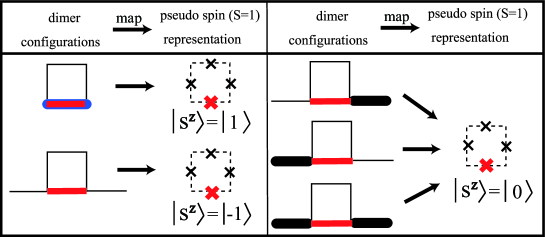
Figure 9: (Color online) Definition of the eigenstates $|$ $\pm$ 1 ⟩  $|$0 ⟩ . $|$1 ⟩ is located on the center of link which is occupied by a dimer, and $|$0 ⟩, $|$-1⟩ are located on the center of links where dimers are absent. $|$-1⟩ is placed on the link where either sides links are not occupied by dimer, and $|$0 ⟩  is the others.

In principle, one could have taken another strategy. Namely, one could have used the $S=1/2$ operators to map a QDM containing large resonance loops and long-range (dimer-dimer) interactions[28] onto an $S=1/2$ (pseudo)spin Hamiltonian with multi-spin- (six-spin and more) and long-range interactions. However, this may lead to the complexity of the interactions and hinder further analyses of the resulting (pseudo-spin) Hamiltonian as well as loss of local Ising gauge invariance. If we use the spin-1 mapping, on the other hand, we can still work within the space of Hamiltonians with only short-range interactions in the sense that the spin-spin interactions exist only among four spins forming a plaquette. In this sense, our EQDM may be thought of as a minimal model of generalized QDMs.

Obviously, the naive state space spanned by the pseudo-spin 1s are much larger than that of the QDM and we have to implement the hardcore dimer constraint in the pseudo-spin language:

$$\sum_{+}\Theta(s_{z})=1\quad\mbox{ with }\;\Theta(x)\equiv\cases{1&\rm{when $0<x$}\\ 0&\rm{when $x\leq 0$}\\ }\;.$$ (17)

When the hardcore constraint is neglected, a single plaquette can take $3^{4}$ different configurations. When the hardcore dimer constraint that at each site only one of the four links emanating from it can be occupied by a dimer and coefficient of diagonal terms ($V_{\rm{EQDM}}$ discussed in the next chapter) into account, then relevant dimer arrangements of a plaquette are restricted to the five patterns shown in Fig. 10. At this point, one may notice that some dimer configurations allowed by the hardcore dimer constraint are missing in the patterns shown in Fig. 10. For instance, a spin-1 state $|s^{z}_{1}\rangle|s^{z}_{2}\rangle|s^{z}_{3}\rangle|s^{z}_{4}\rangle$ with $s^{z}_{1}{=}s^{z}_{2}{=}s^{z}_{3}{=}s^{z}_{4}{=}0$ (a pinwheel-like configuration) is permissible but the coefficient of the diagonal term corresponding to this state is zero as will be seen in eq.(18). A similar argument enables us to drop other constraint-allowed configurations from Fig. 10.

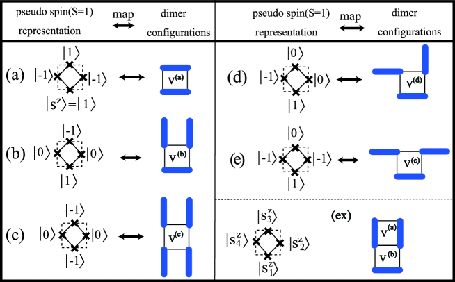
Figure 10: (Color online) Five states allowed by the hardcore constraint and $V_{\rm EQDM}$. Some of the configurations allowed by hardcore constraint have been dropped for the reason that they have zero coefficient in the diagonal part of the Hamiltonian. The pseudo-spins are located on the middle of each link.

Having defined the three $S=1$ pseudo-spin eigenstates in terms of the dimer configurations on an extended (three-bond) cluster, we are at the position of defining the diagonal part of our pseudo-spin Hamiltonian:

$$V_{\rm{EQDM}}=Js_{i}^{z}s_{i+1}^{z}+J^{\prime}s_{i}^{z}s_{i+2}^{z}+\kappa s_{i}^{z}s_{i+1}^{z}s_{i+2}^{z}+\lambda s_{i}^{z}s_{i+1}^{z}s_{i+2}^{z}s_{i+3}^{z}\;,$$ (18)

where the first two are the well-known $J_{1}$-$J_{2}$ interactions[16, 20] and the third one ($\kappa$ term) is a three-spin interaction. Note that this is the most general form which contains all possible short-range many-body spin-spin interactions. The interaction $V_{\rm{EQDM}}$ and the correspondence Fig. 10 determine the coefficients of the diagonal terms as:

$$V_{\rm{EQDM}}^{\rm{(a)}} =-4J+2J^{\prime}+\lambda.$$ (19)

$$V_{\rm{EQDM}}^{\rm{(b)}} =-J^{\prime}.$$ (20)

$$V_{\rm{EQDM}}^{\rm{(c)}} =J^{\prime}.$$ (21)

$$V_{\rm{EQDM}}^{\rm{(d)}} =-J.$$ (22)

$$V_{\rm{EQDM}}^{\rm{(e)}} =-2J+J^{\prime}+\kappa.\$$ (23)

Now it is clear why we have dropped in the previous section several dimer configurations allowed by the hardcore constraint alone (see Fig. 10). In fact, the pinwheel state $|0\rangle_{1}|0\rangle_{2}|0\rangle_{3}|0\rangle_{4}$ mentioned before yields zero when $V_{\rm{EQDM}}$ is applied. For the clarity of the argument, in what follows, we shall restrict our discussion to the diagonal parts of the Hamiltonians, although it is possible to write down the pseudo-spin interactions corresponding to the off-diagonal part of the EQDM.

The mapping is not completed yet at this stage; there exist configurations as shown in Fig.11 that are permitted by the constraint eq.(17) in the spin system, but not in the dimer systems because of the consistency of the definition Fig.9 of the three eigenstates. In order to suppress these forbidden states and realize one-to-one correspondence between the EQDM and the pseudo-spin Hamiltonian, we add the following interaction term to the spin Hamiltonian:

$$V_{\rm{consistency}}=J^{\prime\prime}\sum_{+}\left[s_{j}^{z}s_{k}^{z}-\frac{1}{2}\right]^{2}$$ (24)

with $|J^{\prime\prime}|\gg|J|,|J^{\prime}|$, $J^{\prime\prime}>0$. The summation is taken over all the vertices of the original lattice (see Fig.(11). The auxiliary interaction $V_{\rm{consistency}}$ excludes in the limit $J^{\prime\prime}\nearrow\infty$ the unwanted configurations ([Forbidden]) and selects the allowed ones ([Permitted]) while leaving the latter degenerate:

$$V^{\rm{Forbidden}}_{\rm{consistency}}=\frac{9}{4}J^{\prime\prime}\;,\quad V^{\rm{Permitted}}_{\rm{consistency}}=\frac{1}{4}J^{\prime\prime}.\$$ (25)

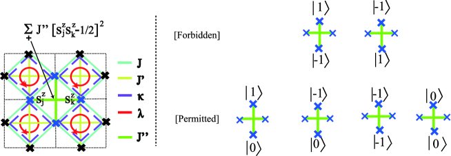
Figure 11: (Color online) [Left] Interactions $V_{\rm EQDM}$ of the pseudo-spin Hamiltonian. dotted dashed lines denote the original square lattice on which dimers are defined and the crosses marks the lattice sites where the pseudo-spins are located. The two-spin interactions $J$ and $J^{\prime}$ are similar to those of the $J_{1}$-$J_{2}$ model and $\lambda$ is the four-spin interaction necessary to realize the RK-point. $J^{\prime\prime}$ forces the one-to-one correspondence between the EQDM and the pseudo $S=1$ Hamiltonian. [Right] Dimer configurations which are forbidden/permitted in the EQDM, due to the definition of the three $S=1$ eigenstates.

This finally establishes the one-to-one mapping between the diagonal part of the EQDM and that of the pseudo-spin Hamiltonian.

The resulting pseudo spin Hamiltonian consists of the diagonal part and the auxiliary interaction $V_{\rm consistency}$ which imposes the consistency condition:

$${V}_{\rm{pseudo}} = {V}_{\rm{EQDM}}+{V}_{\rm{consistency}}$$ (26)

$$= \sum_{\Box}[Js^{z}_{i}s^{z}_{i+1}+J^{\prime}s^{z}_{i}s^{z}_{i+2}+\kappa s^{z}_{i}s^{z}_{i+1}s^{z}_{i+2}+\lambda s^{z}_{i}s^{z}_{i+2}s^{z}_{i+3}s^{z}_{i+4}]$$

$$+\sum_{+}J^{\prime\prime}\left[s^{z}_{j}s^{z}_{k}-\frac{1}{2}\right]^{2}+\rm{(rotations)},$$

where the parameters must satisfy $\mid J^{\prime\prime}\mid$ $\gg$ $\mid J\mid$, $\mid J^{\prime}\mid$. By using the equivalence, the corresponding EQDM is then written down as:

$${\cal H}_{\rm{EQDM}}^{{\rm{diagonal}}}= \sum_{\Box}\Biggl{\{}(-4J+2J^{\prime}+\lambda)\,\bigl{|}\,\raisebox{-4.30554pt}{\includegraphics[scale={0.3}]{VB2.eps}}\,\bigr{\rangle}\bigl{\langle}\,\raisebox{-4.30554pt}{\includegraphics[scale={0.3}]{VB2.eps}}\,\bigr{|}-J\,\Bigl{|}\,\raisebox{-8.61108pt}{\includegraphics[scale={0.3}]{VB5.eps}}\,\Bigr{\rangle}\Bigl{\langle}\,\raisebox{-8.61108pt}{\includegraphics[scale={0.3}]{VB5.eps}}\,\Bigr{|}$$ (27)

$$-J^{\prime}\,\Bigl{|}\,\raisebox{-8.61108pt}{\includegraphics[scale={0.3}]{VB3.eps}}\,\Bigr{\rangle}\Bigl{\langle}\,\raisebox{-8.61108pt}{\includegraphics[scale={0.3}]{VB3.eps}}\,\Bigr{|}+(-2J+J^{\prime}+\kappa)\,\Bigl{|}\,\raisebox{-4.30554pt}{\includegraphics[scale={0.3}]{VB8.eps}}\,\Bigr{\rangle}\Bigl{\langle}\,\raisebox{-4.30554pt}{\includegraphics[scale={0.3}]{VB8.eps}}\,\Bigr{|}$$

$$+J^{\prime}\,\Bigl{|}\,\raisebox{-12.91663pt}{\includegraphics[scale={0.3}]{VB7.eps}}\,\Bigr{\rangle}\Bigl{\langle}\,\raisebox{-12.91663pt}{\includegraphics[scale={0.3}]{VB7.eps}}\,\Bigr{|}+(\rm{h.c.})+(\rm{rotations})+(\rm{reflections})\Biggr{\}}.\$$

As an effective Hamiltonian for Batista and Trugman’s generalized $J_{1}$-$J_{2}$ Heisenberg model (i.e. any states having at least one singlet dimer per plaquette are ground states), the region of each parameters are restricted as

$$V_{\rm{EQDM}}^{\rm{(d)}}<0\Leftrightarrow J>0.$$ (28)

$$V_{\rm{EQDM}}^{\rm{(e)}}<0\Leftrightarrow\kappa<2J-J^{\prime}.$$ (29)

$$V_{\rm{EQDM}}^{\rm{(a)}}+V_{\rm{EQDM}}^{\rm{(b)}}<0,2V_{\rm{EQDM}}^{\rm{(a)}}+V_{\rm{EQDM}}^{\rm{(c)}}>0.$$ (30)

$$\Leftrightarrow 4J-\frac{5}{2}J^{\prime}<\lambda<4J-J^{\prime},J^{\prime}>0.$$ (31)

Introducing the resonance terms

$${\cal H}_{\rm{EQDM}}^{\rm{resonance}} =\sum_{\Box}\Biggl{\{}-t\,\bigl{|}\,\raisebox{-4.30554pt}{\includegraphics[scale={0.3}]{VB1.eps}}\,\bigr{\rangle}\bigl{\langle}\,\raisebox{-4.30554pt}{\includegraphics[scale={0.3}]{VB2.eps}}\,\bigr{|}-t^{\prime}\,\Bigl{|}\,\raisebox{-8.61108pt}{\includegraphics[scale={0.3}]{VB3.eps}}\,\Bigr{\rangle}\Bigl{\langle}\,\raisebox{-8.61108pt}{\includegraphics[scale={0.3}]{VB4.eps}}\,\Bigr{|}-t^{\prime\prime}\,\Bigl{|}\,\raisebox{-12.91663pt}{\includegraphics[scale={0.3}]{VB7.eps}}\,\Bigr{\rangle}\Bigl{\langle}\,\raisebox{-12.91663pt}{\includegraphics[scale={0.3}]{VB9.eps}}\,\Bigr{|}$$ (32)

$$\ \ \ \ \ \ \ \ \ \ \ +(\rm{rotations})+(\rm{reflections})\Biggr{\}}.$$

by hand, we arrive at the EQDM Hamiltonian (2). The coefficient $t$ describes the usual resonance of parallel dimers and the new term $t^{\prime}$ ($t^{\prime\prime}$) moves three (four) dimers on a length-6 (8) loop. Thus, the EQDM is defined as ${\cal H}_{\rm{EQDM}}={\cal H}_{\rm{EQDM}}^{\rm{resonance}}+{\cal H}_{\rm{EQDM}}^{\rm{diagonal}}$. When $t^{\prime},t^{\prime\prime},J,J^{\prime},\kappa=0$, the EQDM reduces to the usual Rokhsar-Kivelson QDM[23]. Furthermore, when $t=J^{\prime}=t^{\prime\prime}=\lambda=\kappa=0$, the phase transition from the columnar VBS to the herringbone, which has been studied by Papanikolaou et al.[28], occurs.

In summary, the requirement that the pseudo-spin Hamiltonian should consist only of short-range interactions enabled us to keep only a restricted class of dimer configurations out of infinitely many ones. This is the greatest advantage of using the pseudo-spin representation of EQDM.

Appendix B Calculation of $t^{\prime}$ resonance effect in dimer smectic

In this section, we outline the second-order calculation of the energy shift (eq.8) caused by the $t^{\prime}$ resonance effect for the dimer smectic. Our calculation closely follows the work of Papanikolaou et al[28].

We treat the small positive resonance terms $t^{\prime}$ as perturbation:

$$V_{\rm{perturb}}^{\rm{t^{\prime}}}= \sum_{\Box}\left\{-t^{\prime}\,\Bigl{|}\,\raisebox{-8.61108pt}{\includegraphics[scale={0.3}]{VB3.eps}}\,\Bigr{\rangle}\Bigl{\langle}\,\raisebox{-8.61108pt}{\includegraphics[scale={0.3}]{VB4.eps}}\,\Bigr{|}+(\rm{rotations})+(\rm{h.c.})\right\}\;.$$ (33)

The first non-trivial contribution of $V_{\rm{perturb}}^{\rm{t^{\prime}}}$ occurs at the second order and the energy shift due to the resonance is given by

$$E_{\rm{resonance}}^{\rm{t^{\prime}}}=\epsilon-{t^{\prime}}^{2}{\sum}^{\prime}_{m}\frac{V_{nm}V_{mn}}{\epsilon_{m}-\epsilon_{n}}+O({t^{\prime}}^{4}),$$ (34)

where $\epsilon$ is the unperturbed energy and the primed summation is over all dimer coverings except the original state. The terms in the sum which give nonzero contribution correspond to states connected to the initial state by a single flipped cluster; these processes are interpreted as brought about by quantum fluctuations.

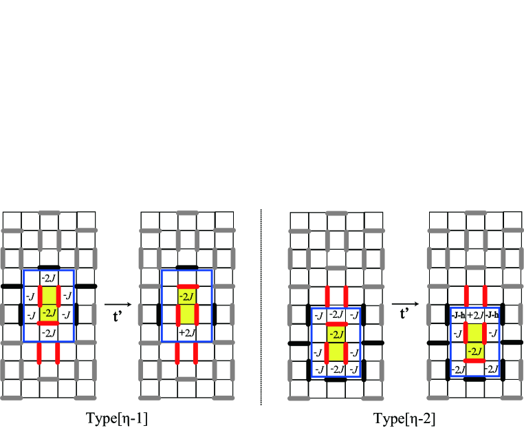
Figure 12: (Color online) Typical intermediate states caused by $t^{\prime}$ resonance term in type-($\eta$) dimer smectic. There are two types of intermediate states (type[$\eta$-1] and [$\eta$-2]). The energies per plaquette are shown too.

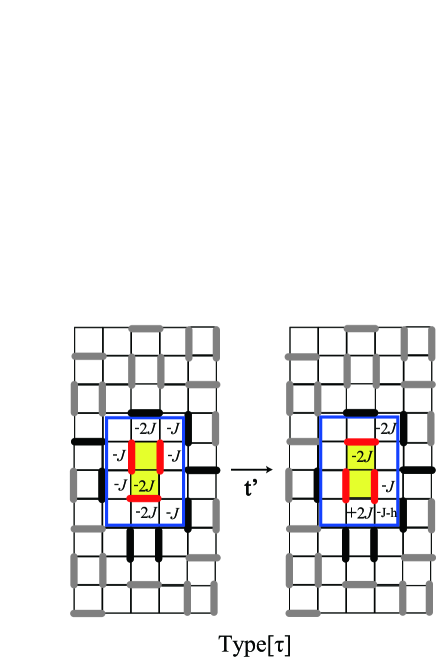
Figure 13: (Color online) Typical intermediate states caused by $t^{\prime}$ resonance term in type-($\tau$) dimer smectic.

Let us consider the energy shift for the dimer smectic case. As has been discussed in section 2.2, dimer smectic has two possible configurations of three neighboring columns (Fig.3) and therefore, we have to treat the two different patterns type-($\eta$) and ($\tau$) carefully.

Type-($\eta$); First, we have to realize furthermore the two different ways (type[$\eta$-1] and type[$\eta$-2] in Fig.12) how a cluster is flipped by $t^{\prime}$. In fact, the intermediate states are different and their energies are different from each other too;

$$\Delta^{\rm{smectic}}_{\rm{t^{\prime}}[\eta{\mathchar 45\relax}1]} =(0)-(-10J)=10J,$$ (35)

$$\Delta^{\rm{smectic}}_{\rm{t^{\prime}[\eta{\mathchar 45\relax}2]}} =(-8J-2h)-(-12J)=4J-2h.$$ (36)

Type-($\tau$); we do not have to worry about the above difference, because both cases give the same results. The energy shift is as below (Fig.13):

$$\Delta^{\rm{smectic}}_{\rm{t^{\prime}[\tau]}} =(-4J-h)-(-11J)=7J-h.$$ (37)

Putting all these effects of the resonance $t^{\prime}$ together, we obtain the energy shift caused by $t^{\prime}$-resonance of the dimer smectic as

$$\Delta E_{\rm{t^{\prime}}\rm{resonance}}^{\rm{smectic}} =-\frac{t^{\prime 2}}{4J-2h}N_{\eta}\frac{N_{y}}{3}-\frac{t^{\prime 2}}{10J}N_{\eta}\frac{N_{y}}{3}-\frac{t^{\prime 2}}{7J-h}N_{\tau}\frac{2N_{y}}{3}.$$ (38)

The calculation goes similarly for $t$ and $t^{\prime\prime}$ as well and collecting all the terms, we obtain the energy of the dimer smectic with all resonance effects as eq.(8).

References

References

- [1] P.W.Anderson. Mater.Res.Bull, 8:153, 1973.
- [2] P.Fazekas and P.W.Anderson. Philos.Mag, 30:23, 1974.
- [3] P.W.Anderson. Science, 235:1196, 1987.
- [4] H.Tasaki and M.Kohmoto. Phys.Rev. B, 42:2547, 1990.
- [5] K.Takano and K.Sano. Phys.Rev. B, 39:7367, 1989.
- [6] N.Read and B.Chakraborty. Phys.Rev. B, 40:7133, 1989.
- [7] M.Kohmoto and Y.Shapir. Phys.Rev. B, 37:9439, 1988.
- [8] K.S.Raman, M.Moessner, and S.L.Sondhi. Phys.Rev. B, 72:064413, 2005.
- [9] R.Moessner and S.L.Sondhi. Phys.Rev. B, 68:184512, 2003.
- [10] M.P.Gelfand, R.R.P.Singh, and D.A.Huse. Phys.Rev. B, 40:10801, 1989.
- [11] R.Moessner, S.L.Sondhi, and P.Chandra. Phys. Rev. Lett, 84:4457, 2000.
- [12] R.Moessner and S.L.Sondhi. Phys.Rev. B, 63:224401, 2001.
- [13] C.Lhuillier. arXiv cond-mat/05024641.
- [14] C.K.Majumdar and D.K.Ghosh. J.Math.Phys, 10:1399, 1969.
- [15] B.S.Shastry and B.Sutherland. Physica B, 108:1069, 1981.
- [16] P.Chandra and B.Doucot. Phys.Rev. B, 38:9335, 1988.
- [17] R.Melzi, P.Carretta, A.Lascialfari, M.Mambrini, M.Troyer, P.Millet, and F.Mila. Phys.Rev. Lett, 85:1318, 2000.
- [18] O.P.Sushkov, J.Oitmaa, and Zheng Weihong. Phys.Rev. B, 63:104420, 2000.
- [19] Jaan Oitmaa, Chris Hamer, and Weihong Zheng. Series Expansion Method for strongly interacting Lattice Models. Cambridge University Press, 2006.
- [20] H.Nishimori and Y.Saika. J.Phys.Soc.Jpn, 58:4454, 1990.
- [21] P.Chandra, P.Coleman, and A.I.Larkin. Phys.Rev. Lett, 64:88, 1990.
- [22] N.Read and S.Sachdev. Phys.Rev. Lett, 62:1694, 1989.
- [23] D.S.Rokhsar and S.A.Kivelson. Phys.Rev. Lett, 61:2376, 1988.
- [24] G.Misguich and C.Lhuillier. Two-dimensional quantum antiferromagnets, chapter 5, page 229. World-Scientific, 2005.
- [25] R.Moessner and K.S.Raman. arXiv cond-mat/08093051.
- [26] A. Ralko, M. Mambrini, and D. Poilblanc. Phys.Rev.B, 80:184427, 2009.
- [27] David Schwandt and Matthieu Mambriniand Didier Poilblanc. Phys.Rev.B, 81:214413, 2010.
- [28] S.Papanikolaou, K.S.Raman, and E.Fradkin. Phys. Rev. B, 75:094406, 2007.
- [29] V.I.Pokrovsky and A.L.Talapov. Zh.Eksp.Teor.Fiz, 75:1151, 1978.
- [30] A.B.Harris, C.Micheletti, and J.M.Yeomans. Phys.Rev. B, 52:6684, 1995.
- [31] P.Bak and J.V.Boehm. Phys.Rev. B, 21:5297, 1980.
- [32] M.E.Fisher and W.Selke. Phys.Rev.Lett, 44:1502, 1980.
- [33] A.B.Harris, C.Micheletti, and J.M.Yeomans. Phys.Rev.Lett, 74:3045, 1995.
- [34] C.D.Batista and S.A.Trugman. Phys.Rev.Lett, 91:217202, 2004.
- [35] P.W. Leung, K.C. Chiu, and K.J. Runge. Phys.Rev. B, 54:12938, 1996.
- [36] O.F.Syljuasen. Phys.Rev. B, 73:245105, 2006.
- [37] A. Ralko, D. Poilblanc, and R. Moessner. Phys.Rev.Lett., 100:037201, 2008.
- [38] M.Muller, T.Vecua, and H.J.Mikeska. Phys.Rev. B, 66:134423, 2002.
- [39] B. Normand Z. Nussinov, C. D. Batista and S. A. Trugman. Phys.Rev. B, 75:094411, 2007.
- [40] A. Chubukov. Phys.Rev.Lett, 69:832, 1992.
- [41] R. Moessner and J.T. Chalker. Phys.Rev. B, 58:12049, 1998.
- [42] Michael Levin and T. Senthil. Deconfined quantum criticality and N[e-acute]el order via dimer disorder. Phys. Rev. B, 70(22):220403, 2004.
- [43] J.Villain, R.Bidaux, J.P.Carton, and R.Conte. J.Phys.(Paris), 41:1263, 1980.
- [44] E.F. Shender. Sov.Phys.JETP, 56:178, 1982.
- [45] E. Fradkin S.A. Kivelson and V.J. Emery. Nature, 393:550, 1998.
- [46] S.A. Kivelson V.J. Emery, E. Fradkin and T.C. Lubensky. Phys.Rev.Lett., 85:2160, 2000.
- [47] T.C. Lubensky C.S. O’Hern and J. Toner. Phys.Rev.Lett., 83:2745, 1999.
- [48] R.R.P. Singh O.A. Starykh and G.C. Levine. Phys.Rev.Lett., 88:167203, 2002.
- [49] J-B. Fouet P. Sindzingre and C. Lhuillier. Phys.Rev. B, 66:174424, 2002.
- [50] R.Moessner, S.L.Sondhi, and E.Fradkin. Phys. Rev. B, 65:024504, 2001.