Topics on Galactic Chemical Evolution

Abstract:

I discuss three different topics in Galactic chemical evolution: the ”puzzling” absence of any observational signature of secondary elements ; the building of the Galactic halo in the framework of hierarchical galaxy formation, as evidenced from its metallicity distribution ; and the potentially important role that radial migration may play in the evolution of galactic disks, according to recent studies.

1 The elusive secondary elements

In the field of galactic chemical evolution primary elements are those produced from the initial (essentially primordial) H and He entering a star at its formation, while secondary elements are those formed from all other elements (metals) entering the star. Thus, the yields of primary elements are independent of the stellar metallicity, while those of secondaries increase with it. As a result, the secondary/primary ratio is expected to increase linearly with metallicity. Typical examples of primaries are the $\alpha$ nuclides (¹²C, ¹⁶O, ²⁰Ne, etc.) as well as ⁵⁶Fe, while it was traditionally thought that ¹⁴N (produced from initial C and O through the CNO cycle in H-burning), or the s-elements (produced by n-captures on seed Fe nuclei) are typical secondaries. It turns out, however, that neither those elements, nor any other (up to now) shows the expected typical behaviour of secondaries. In other terms, the concept of secondary element remains only theoretical up to now, with no observational substantiation. In some cases, we (think that we) understand the relevant observations, but in others the situation is still unclear.

1.1 The quest for primary Nitrogen

The behaviour of N as primary (i.e. [N/Fe]$\sim$0) was known for sometime, but it was recently confirmed from VLT mesurements (Spite et al. 2005) down to the realm of very low metallicities ([Fe/H]$\sim$-3, see Fig. 1 middle right). For a long time, the only known source of primary N was Hot Bottom Burning (HBB) in massive AGB stars. Such stars (typical mass $M\sim$8 M_⊙) have lifetimes $\sim$10⁸ yr, considerably longer than those of typical SNII progenitors (20 M_⊙ stars living for $\sim$10⁷ yr); thus, it is improbable, albeit not impossible that that they contributed to the earliest enrichment of the Galaxy with N. On the other hand, massive stars were thought to produce N only as secondary (from the initial CNO) and not to be at the origin of the observed behaviour.

Rotationally induced mixing in massive stars changed the situation considerably: N is now produced by H-burning of C and O produced inside the star. As in the case of HBB in massive AGBs, N is produced after mixing of protons in He-rich zones, where ¹²C originates from the 3-$\alpha$ reaction, i.e. N is produced as primary; it is subsequently ejected to the ISM mostly by the winds of those massive stars. Stellar models rotating at 300 km/s (typical velocity for solar metallicity stars) at all metallicities, did not provide enough primary N at low metallicities to explain the data (Prantzos 2003a and Fig. 1, middle right). Assuming that low metallicity massive stars were rotating faster than their high-metallicity present-day counterparts (at 800 km/s) leads to a large production of primary N, even at low $Z$ and allows one to explain the data (e.g. Chiappini et al. 2006 and Fig. 1, middle right). Thus, there appears to be a ”natural” solution to the problem of early primary N, which may impact on other isotopes as well (e.g. ¹³C, produced in a similar way). Even more important, it may also impact on the next item in the list, namely the evolution of beryllium.

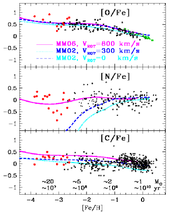
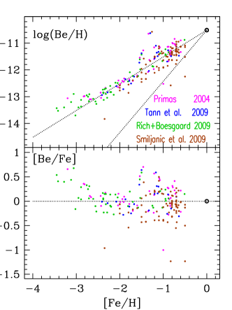
Figure 1: Left: Evolution of C, N and O vs Fe/H. Solid (purple) curves correspond to yields of fast rotating stars at low metallicity and reproduce the observed early behaviour of N. Evolutionary timescales corresponding to the metallicity scale and masses of stars dying in those timescales appear in the lower panel.Right: Observations of Be/H and Be/Fe vs Fe/H; the two dotted lines correspond to primary and secondary behaviour, respectively.

1.2 The quest for primary Be

Observations of halo stars in the 90s revealed a linear relationship between Be/H and Fe/H (Gilmore et al. 1991, Ryan et al. 1992) as well as between B/H and Fe/H (Duncan et al. 1992). That was unexpected, since Be and B were thought to be produced as secondaries, by spallation of the increasingly abundant CNO nuclei of the ISM during the propagation of protons and aplhas of Galactic Cosmic rays (GCR). The only way to produce primary Be is by assuming that it is produced by the fragmentation of the CNO nuclei of GCR, as they hit the p and $\alpha$ of the ISM and that GCR have always the same CNO content (Duncan et al. 1992); other efforts to enhance the early production of Be, by e.g. invoking a better confinement - and thus, higher fluxes - of GCR in the early Galaxy (Prantzos et al. 1993) only partially succeeded. The reason was clearly revealed by the “energetics argument” put forward by Ramaty et al. (1997): if SN are the main source of GCR energy, there is a limit to the amount of light elements produced per SN, which depends on GCR and ISM composition. If the metal content of both ISM and GCR is low, there is simply not enough energy in GCR to keep the Be yields constant. The only possibility to have $\sim$constant LiBeB yields is by assuming that the “reverse” component of GCR (fast CNO nuclei) is primary, i.e. that GCR have a $\sim$constant metallicity (Fig. 2 in Prantzos 2010). This has profound implications for our understanding of the GCR origin. It should be noted that before those observations, no one would have the idea to ask “what was the GCR composition in the early Galaxy?”.

For quite some time it was thought that GCR originate from the average ISM, where they are accelerated by the forward shocks of SN explosions; this can only produce secondary Be. A $\sim$constant abundance of C and O in GCR can “naturally” be understood if SN accelerate their own ejecta, trough their reverse schock (Ramaty et al. 1997). However, the absence of unstable ⁵⁹Ni (decaying through e^- capture within 10⁵ yr) from observed GCR suggests that acceleration occurs $>$10⁵ yr after the explosion (Wiedenbeck et al. 1999) when SN ejecta are presumably already diluted in the ISM.

Higdon et al. (1998) suggested that GCR are accelerated out of superbubbles (SB) material, enriched by the ejecta of many SN as to have a large and $\sim$constant metallicity. In this scenario, it is the forward shocks of SN that accelerate material ejected from other, previously exploded SN (see Binns et al. 2005, Rauch et al. 2009). The SB scenario suffers from several drawbacks (Prantzos 2010) which, however, may not be lethal. Still, it is hard to imagine that SB have always the same average metallicity, especially during the early Galaxy evolution, where metals were easily expelled out of the shallow potential wells of the small sub-units forming the Galactic halo.

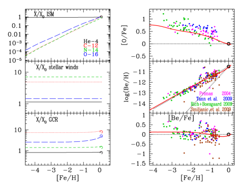
Figure 2: Left: Evolution of the chemical composition (in corresponding solar abundances) of He-4 (solid), C-12 (dotted), N (short dashed) and O (long dashed)in: ISM (top), massive star winds (middle) and GCR (bottom). Dots in lower panel indicate estimated GCR source composition (from Elison et al. 1997). Right: Evolution (solid curves of O/Fe (top), Be/H (middle) and Be/Fe (bottom); dotted lines indicate solar values in top and bottom panels, primary and secondary Be in middle panel.

A different explanation for the origin of GCR, is proposed in Prantzos (2010). He notices that rotating massive stars display substantial mass loss down at very low (or even zero) metallicities (see previous section). Assuming that GCR are accelerated when the forward shocks of SN propagate into the previously ejected envelopes of rotating massive stars (partially mixed with the surrounding ISM), one may then calculate the evolution of the ISM and GCR composition (Fig. 2, left). It is found that the resulting Be evolution nicely fits the data (Fig. 2, right); it is the first time that such a calculation is performed not by assuming a given GCR composition, but by calculating it in a (hopefully) realistic way.

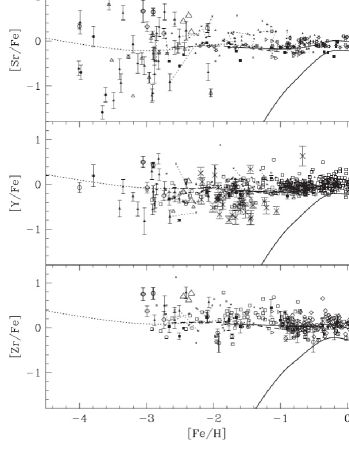
Figure 3: Evolution of Sr, Y and Zr in the Galaxy (halo and solar neighborhood): observations vs a model involving s-process from low and intermediate mass stars (solid curves) and a putative n-process (dashed curves). From Travaglio et al (2004).

1.3 The early appearance of s-elements

The products of slow n-capture (s-process) were traditionally thought to behave as secondaries. However, various theoretical arguments suggest that this cannot be true in most cases and current uncertainties prevent from making sound theoretical predictions for the behaviour of those elements.

1) Solar system s-elements have a primary contribution $f_{r}=Y_{r}/(Y_{r}+Y_{s})$ (where $Y_{s}$ and $Y_{r}$ are the corresponding yields) from the r-process; thus, for an s-element $X$, a ”floor” in the [X/Fe] ratio is expected below some metallicity $Z$ (Truran 1981). But the evolution of $f_{r}$ with $Z$ is poorly determined, because of the unknown evolution of $Y_{s}$ (while $Y_{r}$ is expected to evolve roughly as the oxygen yield $Y_{O}$, at least at late times).

2) $Y_{s}(Z)$ depends on: i) the behaviour of the ”neutron economy trio” (sources - poisons - seed nuclei) with metallicity (Prantzos et al. 1990); for instance, the behaviour of the n-source ¹³C($\alpha$,n) is different from the one of ²²Ne($\alpha$,n) and ii) the mass range of the s-element sources (stars with $M\sim$1.5-3 M_⊙, with lifetimes from a few 10⁸ to a few 10⁹ yr for the ”main” s-component, but massive stars for the ”weak” s-component); since the yields of individual stars $y(M,Z)$ are unknown, the behaviour of the global yield $Y_{s}(Z)$ (averaged over the IMF) is unknown also.

In the case of heavy s-elements, like Ba, the observed behaviour of e.g. the Ba/Eu ratio (Eu being an almost pure r-element) can be explained as resulting from a pure r- contribution below [Fe/H]$\sim$-1.5 (where [Ba/Eu]$\sim$const.$\sim$-0.6) and a stronger (but not monotonically increasing) contribution from the s-process in intermediate mass stars above that value (see Travaglio et al. 1999). However, the situation appears much more difficult in the case of the light s-elements Sr, Y and Zr, which behave exactly as Fe (i.e. the [X/Fe] ratio is $\sim$constant down to the lowest metallicities). Since the r- contribution to the solar system abundances of those elements is small, Travaglio et al. (2004) suggested the operation of an unknown neutron capture process (called n-process) of primary nature in massive stars at low metallicities.

One might think that a ”natural” site for that process may be ²²Ne($\alpha$,n) in core He-burning in massive rotating stars: indeed, as stressed in Sec. 1.1, primary ¹⁴N is produced in those stars, and the amount remaining in the He-burning -zones is turned mostly into $primary^{22}$Ne early in He-burning. However, since both the neutron source ²²Ne and the main neutron poisons ²⁵Mg and ²²Ne are primary, the s-process in the Sr-Zr region turns out to be secondary (scaling with the Fe seed abundance), as shown in Pignatari et al. (2008) with a 25 M_⊙ model of rotating star at metallicities [Fe/H]=-3 and -4, respectively. Thus, the observed primary behaviour of Sr, Y and Zr at low metallicity remains unexplained at present.

2 The MW halo in cosmological context

The metallicity distribution (number of stars per unit metallicity interval) of a galaxian system gives valuable information about its history, and in particular, the occurence of gaseous flows (infall, outflow). The regular shape of the metallicity distribution of the Milky Way (MW) halo can readily be explained by the simple model of galactic chemical evolution (GCE) with outflow, as suggested by Hartwick (1976). However, that explanation lies within the framework of the monolithic collapse scenario for the formation of the MW (Eggen, Lynden-Bell and Sandage, 1962). Several attempts to account for the metallicity distribution of the MW halo in the modern framework (hierarchical merging of smaller components, hereafter sub-haloes) were undertaken in recent years through numerical simulations (Bekki and Chiba 2001; Salvadori et al. 2007). Independently of their success or failure in reproducing the observations, such models provide little or no physical insight into the physical processes that shaped the metallicity distribution of the MW halo. Why is its metallicity distribution so well described by the simple model with outflow (which refers to a single system)? And what determines the peak of the metallicity distribution at [Fe/H]=$\sim$–1.6, which is (successfully) interpreted in the simple model by a single parameter (the outflow rate) ? Here we present an attempt to built the halo metallicity distribution analytically (Prantzos 2008a) in the framework of the hierarchical merging paradigm.

2.1 The halo metallicity distribution and the simple model

The halo metallicity distribution is nicely described by the simple model of GCE, in which the metallicity $Z$ is given as a function of the gas fraction $\mu$ as $Z\ =\ p\ ln(1/\mu)\ +Z_{0}$, where $Z_{0}$ is the initial metallicity of the system and $p$ is the yield (metallicities and yield are expressed in units of the solar metallicity Z_⊙). If the system evolves at a constant mass (closed box), the yield is called the true yield, otherwise (i.e. in case of mass loss or gain) it is called the effective yield. The differential metallicity distribution (DMD) is:

$${{d(n/n_{1})}\over{d(logZ)}}\ =\ {{{\rm ln10}}\over{1-{\rm exp}\left(-{{Z_{1}-Z_{0}}\over{p}}\right)}}\ {{Z-Z_{0}}\over{p}}\ {\rm exp}\left(-{{Z-Z_{0}}\over{p}}\right)$$ (1)

where $Z_{1}$ is the final metallicity of the system and $n_{1}$ the total number of stars (having metallicities $\leq Z_{1}$). This function has a maximum for $Z-Z_{0}=p$, allowing one to evaluate easily the effective yield $p$ if the DMD is observed. In the case of outflow at a rate $F\ =\ k\ \Psi$ (where $\Psi$ is the Star Formation Rate or SFR) one obtains $k\ =\ (1-R)\ (p_{True}/p_{Halo}-1)$, where $R\sim$0.35 is the return mass fraction of the system, $p_{True}$ and $p_{Halo}$ the observationnaly determined yields in the bulge (fitetd with a closed box model) and the halo, respectively. The DMD of the MW halo is nicely fit with a simple outflow model with $k\sim$7-8.

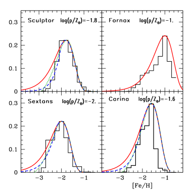
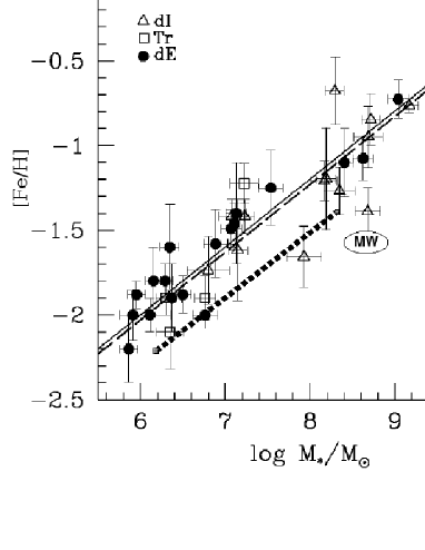
Figure 4: left: Metallicity distributions of dwarf satellites of the Milky Way. Data are in histograms (from Helmi et al. 2006). Solid curves indicate the results of simple GCE models with outflow proportional to the star formation rate; the corresponding effective yields (in Z_⊙) appear on top right of each panel. Dashed curves are fits obtained with an early infall phase, while dotted curves are models with an initial metallicity log$(Z_{0})\sim$–3; both modifications to the simple model (i.e. infall and initial metallicity) improve the fits to the data. Right: Stellar metallicity vs stellar mass for nearby galaxies; data and model (upper curves) are from Dekel and Woo (2003), with dI standing for dwarf irregulars and dE for dwarf ellipticals. The thick dotted line represents the effective yield of the sub-haloes that formed the MW halo according to this work (i.e. with no contribution from SNIa, see Sec. 3.2). The MW halo, with average metallicity [Fe/H]=–1.6 and estimated mass $\sim$4x10⁸ M_⊙ falls below both curves.

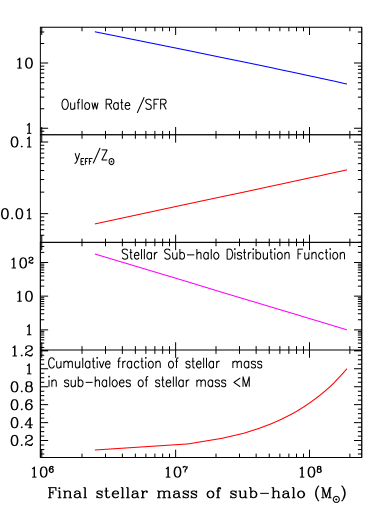
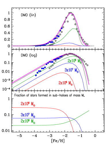
Figure 5: Left:Properties of the sub-haloes as a function of their stellar mass, empirically derived as discussed in Sec. 3. From top to bottom: Outflow rate, in units of the corresponding star formation rate; Effective yield, in solar units; Distribution function; Cumulative fraction of stellar mass contributed by the sub-haloes. The total mass of the MW halo is 4 10⁸ M_⊙. Right:Top and middle panels: Differential metallicity distribution (in lin and log scales, respectively) of the MW halo, assumed to be composed of a population of smaller units (sub-haloes). The individual DMDs of a few sub-haloes, from 10⁶ M_⊙ to 4 10⁷ M_⊙, are indicated in the middle panel, as well as the sum over all haloes (solid upper curves in both panels, compared to observations). Dotted curves in top and middle panels indicate the results of the simple model with outflow (same as in Fig. 1). Because of their large number, small sub-haloes with low effective yields contribute the largest fraction of the lowest metallicity stars, while large haloes contribute most of the high metallicity stars (bottom panel). Figure from Prantzos (2008).

2.2 The halo DMD and hierarchical merging

Assuming that the MW halo was formed by the merging of smaller units (”sub-haloes”), one has to know: a) the DMD of each sub-halo and b) the number distribution of the sub-haloes $dN/dM$. Prantzos (2008a) assumed that the DMD of each sub-halo had a DMD described by the simple model with an appropriate effective yield. This assumption is based on recent observations of the dwarf spheroidal (dSph) satellites of the Milky Way. The DMDs of four nearby dSphs (Helmi et al. 2006) are displayed as histograms in Fig. 4 (left), where they are compared to the simple model with appropriate effective yields (solid curves). The effective yield in each case was simply assumed to equal the peak metallicity (Eq. 1.1). It can be seen that the overall shape of the DMDs is quite well fitted by the simple models. This is important, since i) it strongly suggests that all DMDs of small galaxian systems can be described by the simple model and ii) it allows to determine effective yields by simply taking the peak metallicity of each DMD. Observations suggest that the effective yield is a monotonically increasing function of the galaxy’s stellar mass $M_{*}$ (Fig. 4 right). In the case of the progenitor systems of the MW halo, however, the effective yield must have been lower, since SNIa had not time to contribute (as evidenced by the high $\alpha$/Fe$\sim$0.4 ratios of halo stars), by a factor of about 2-3. We assume then that the effective yield of the MW halo components $p(M_{*})$ (accreted satellites or sub-haloes) is given (in Z_⊙) by the thick dotted curve in Fig. 4 (right). The stellar mass $M_{*}$ of each of the sub-haloes should be $M_{*}<M_{H}$ where $M_{H}$ is the stellar mass of the MW halo ( $M_{H}$= 4$\pm$0.8 10⁸ M_⊙, e.g. Bell et al. 2007).

Hierarchical galaxy formation scenarios predict the mass function of the dark matter sub-haloes which compose a dark matter halo at a given redshift. Several recent simualtions find $dN/dM_{D}\ \propto\ M_{D}^{-2}$ (e.g. Giocoli et al. 2008). In our case, we are interested in the mass function of the stellar sub-haloes, and not of the dark ones. Considering the effects of outflows on the baryonic mass function, Prantzos (2008a) finds that $dN/dM_{*}\ \propto\ M_{*}^{-1.2}$, i.e. the distribution function of the stellar sub-haloes is flatter than the distribution function of the dark matter sub-haloes.

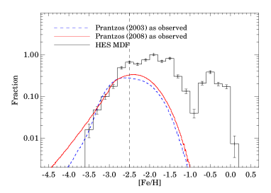
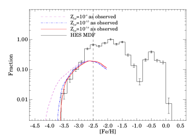
Figure 6: Comparison of the MDF of main sequence and turn-off halo stars of the HES sample to theoretical predictions Left:. Comparison to Prantzos (2003b) and Prantzos(2008a). Right: Comparison to Salvadori et al. (2007). Figure from Li et al. (2010).

The main properties of the sub-halo set constructed in this section appear in Fig. 5 (left) as a function of the stellar sub-halo mass $M_{*}$. The resulting total DMD is obtained as a sum over all sub-haloes:

$$\frac{d(n/n_{1})}{d(logZ)}\ =\ \int_{M_{1}}^{M_{2}}\ \frac{d[n(M_{*})/n_{1}(M_{*})]}{d(logZ)}\ \frac{dN}{dM_{*}}\ M_{*}\ dM_{*}$$ (2)

The result appears in Fig. 5 (right, with top panel in linear and middle panel in logarithmic scales, respectively). It can be seen that it fits the observed DMDs at least as well as the simple model à la Hartwick. In summary, under the assumptions made here, the bulk of the DMD of the MW halo results naturally as the sum of the DMDs of the component sub-haloes and can be understood analytically. It should be noted that all the ingredients of the analytical model are taken from observations of local satellite galaxies, except for the adopted mass function of the sub-haloes (which results from analytical theory of structure formation plus a small modification to account for the role of outflows).

Besides the shape of the bulk of the halo DMD, its low metallicity tail offers valuable clues as to the early period of halo formation and metal enrichment. Recent analysis of the HES data, for $\sim$1700 giant stars (Schörck et al. 2009) and for $\sim$700 turn-off stars (Li et al. 2010, Fig. 6) seem to suggest a sharp decline in star numbers below [Fe/H]$\sim$–3.5, which could be interpreted as evidence for halo formation from gas pre-enriched to that value (e.g. Salvadori et al. 2007). However, the situation may be more complex (”dual” halo structure, with unknown relative contributions from an inner, metal-rich and an outer, metal-poor halo, Carollo et al. 2007) and small number statistics at such low metallicities prevent any definitive conclusions yet. Fortcoming studies (SEGUE-2, APOGEE, LAMOST) are expected to clarify the situation in that metallicity range.

3 Radial mixing in the Milky way disk

In classical studies of GCE it is explicitly assumed that the system may be ”open” as far as its gas is concerned (allowing for e.g. infall, outflow or radial inflows) but it is ”closed” regarding its stars: once formed they remain in the system and their properties (especially those of long-lived ones: metallicity distribution, age-metallicity relation) can help us to reconstruct the history of the system. This paradigm started changing in recent years, making the interpretation of stellar data more difficult (requiring combined studies of chemistry and kinematics), but also more enriching, opening new perspectives.

The idea that stars in a galactic disk may diffuse to large distances along the radial direction (i.e to distances larger than allowed by their epicyclic motions) was proposed by Wielen et al. (1996). They suggested that some of the peculiar chemical properties of the Sun may be explained by the assumption that it was born in the inner Galaxy (i.e. in a high metallicity region, in view of the galactic metallicity gradient) and subsequently migrated outwards. They treated the hypothetical radial migration phenomenologically, acknowledging that the basic mechanism for the gravitational perturbations of stellar orbits is not understood.

Sellwood and Binney (2002, herefter SB02) convincingly argued that stars can migrate over large radial distances, due to continuous resonant interactions with transient spiral density waves at co-rotation. Such a migration alters the specific angular momentum of individual stars, but affects very little the overall distribution of angular momentum and thus does not induce important radial heating of the disk. Because high-metallicity stars from the inner (more metallic and older) and the outer (less metallic and younger) disc are brought in the solar neighborhood, SB02 showed with a simple toy model that considerable scatter may result in the local age-metallicity relation, not unlike the one observed by Edvardsson et al. (1993); see also Prantzos (2008b).

Another obvious implication of the radial migration model of SB02 concerns the flattening of the stellar metallicity gradient in the galactic disk. That issue was quantitatively explored in Lepine et al. (2003), who considered, however, the corotation at a fixed radius (contrary to SB02). As a result, the gravitational interaction bassically removes stars from the local disk, ”kicking” them inwards and outwards. The abundance profile (assumed to be initially exponential) is little affected in the inner Galaxy, but some flattening is obtained in the 8-10 kpc region. The authors claim that such a flattening is indeed observed (using data of planetary nebulae by Maciel and Quireza 1996) but modern surveys do not find it.

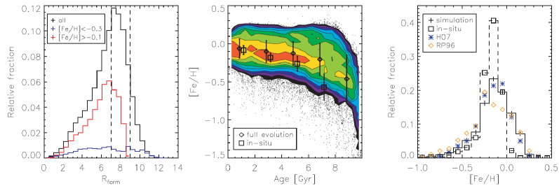
Figure 7: Properties of stars in the solar neighborhood. Left: Histogram of birth radii for stars that end up in the solar neighborhood on nearly circular orbits. The black, red, and blue lines represent all, metal-rich, and metal-poor stars, respectively. Middle: The age-metallicity relation: color contours represent relative particle densities where point density is high. Diamonds and error bars indicate mean values and dispersion, respectively. Squares show the AMR if stars are assumed to remain in situ. A small horizontal offset is applied to the two sets of symbols for clarity. Right: Metallicity distribution function (MDF): the simulated distribution is shown with the solid black histogram; diamonds and asterisks show data from Rocha-Pinto and Maciel (1996) and Holmberg et al. (2007), respectively. The dashed histogram is the MDF if stars are assumed to remain in situ (from Roskar et al. 2008).

On the basis of kinematics and abundance observations of a large sample of local stars Haywood (2008) argues that most of the metal rich stars in the solar neighborhood originate from the inner disk and most of the metal poor ones from the outer disk, and suggests that the local disk started its evolution with a considerably high metallicity of [Fe/H]$\sim$-0.2. However, such a large pre-enrichment of the thin disk is difficult to accept, because no other local component of the Galaxy is massive enough to enrich to such a high level the massive thin disk. Independently, however, of his far-reaching conclusions, Haywood (2008) presents convincing arguments that the local stellar population shows evidence for substantial contamination with stars from other Galactic regions. This idea has profound implications for galactic chemical evolution studies, since it implies that observations of a stellar population in a given region cannot be used to derive the history of that region: the history of adjacent (and even remote) regions has to be considered as well.

Building on the ideas of SB02, Schoenrich and Binney (2009, SB09) presented a full scale semi-analytic model for the chemical evolution of the Milky Way disk, including several ingredients: gaseous infall, radial inflow of gas along the disk, churning of stars and cold (but not hot) gas and blurring of stars. The model has a rather large number of parameters and assumptions and finds excellent agreement with each and every observable in the solar neighborhood (including shape and scatter in age-metallicity relation, G-dwarf metallicity distribution, kinematics of thin and thick disk etc.). In particular, the properties of the thick disk are ”naturally” found in this model as a result of secular evolution, with no need to invoke galactic mergers.

Numerical (N-body + SPH) simulations of Roskar et al. (2008) have already shown that extensive radial mixing may occur in disk galaxies, due to the action of spiral arms, and that it may help explaining observed properties of the solar neighborhood (Fig. 7). Recent simulations of Loebman et al. (2010) lend support to the idea of thick disk resulting from secular evolution (albeit with substantial differences on some observables with respect to SB09): the local thick disk results from stars migrated from the inner disk, retaining their (high) vertical velocity dispersions but found in the lower gravitational potential of the solar neighborhood. Finally, Minchev and Famaey (2010) find that the galactic bar, in conjunction with the spiral arm potential, may play an efficient role in accelerating radial migration of stars.

Although it is rather early to say whether the global picture of the Milky Way evolution (involving an inside-out disk formation) will change drastically, it is clear that those works open new and promising perspectives in GCE studies.

Acknowledgements: I am grateful to the organizers of NiCXI for their invitation and financial support.

References

- [1] Bekki, K., Chiba, M., 2001, ApJ 558, 666
- [2] Bell, E., Zuker, D, Belokurov, V., 2008, ApJ 680, 295
- [3] Binns, W. R., Wiedenbeck, M. E., Arnould, M. et al., 2005, ApJ 634, 351
- [4] Carollo, D., Beers, T., Lee Y., et al., 2007, Nature 450, 1020
- [5] Chiappini, C., Hirschi, R., Meynet, G., et al., 2006, A&A 449, L27
- [6] Edvardsson, B., Andersen, J., Gustaffson B., et al., 1993, A&A 275, 101
- [7] Dekel, A., Woo, J., 2003, MNRAS 344, 1131
- [8] Diemand, J., Kuhlen, M., Madau, P., 2007, ApJ 667, 859
- [9] Duncan, D., Lambert, D., Lemke, M., 1992, ApJ 584, 595
- [10] Feltzing, S., Holmberg, J., Hurley, J. R., A&A 377, 911
- [11] Font, A., Johnston, K., Bullock, J., Robertson, B., 2006, ApJ, 638, 585
- [12] Gilmore, G., Gustafsson, B., Edvardsson, B., Nissen, P. E., 1992, Nature 357, 379
- [13] Giocoli, C., Pieri, L., Tormen, G. 2008, MNRAS 387, 689
- [14] Goswami, A., Prantzos, N., 2000, A&A 359, 151
- [15] Hartwick, F., 1976, ApJ 209, 418
- [16] Haywood, M., 2008, MNRAS 388, 1175
- [17] Heller, C., Shlosman, I., Athanassoula, E., 2007, ApJ 671, 226
- [18] Helmi, A., Irwin, M., Tolstoy, E., et al., 2006, ApJ 651, L121
- [19] Higdon, J., Lingenfelter, R., Ramaty, R., 1998, ApJ 509, L33
- [20] Holmberg, J., Norström, B., Andersen, J., 2007, A&A 475, 519
- [21] Kroupa, P., 2002, Science 295, 82
- [22] Lepine, J. R.. D., Acharova, I. A., Mishurov, Y. N., 2003, ApJ 589, 210
- [23] Loebman, S. R.; Roskar, R., Debattista, V. P., et al., 2010, arXiv:1009.5997
- [24] Li, H. N., Christlieb, N., Schrck, T., 2010, A&A 521, 10
- [25] Minchev, I., Famaey, B., 2010, ApJ 722, 112
- [26] Nordström, B., Mayor, M., Andersen, J., et al., AA418, 989
- [27] Olive, K., Prantzos, N., Scully, S., Vangioni-Flam, E., 1994, ApJ 424, 666
- [28] Pignatari, M., Gallino, R., Meynet, G., et al., 2008, ApJ 687, L95
- [29] Prantzos, N., 2003a, in ”CNO in the Universe”, Edited by C. Charbonnel, D. Schaerer, and G. Meynet. ASP Conference Series, Vol. 304, p.361
- [30] Prantzos, N. 2003b, A&A 404, 211
- [31] Prantzos, N., 2008a, A&A 489, 525
- [32] Prantzos, N., 2008b, in ”The Galaxy Disk in Cosmological Context”, IAU Symposium 254. p. 381-392
- [33] Prantzos, N., 2010, in ”Light Elements in the Universe”, IAU Symposium 268, p. 473-482
- [34] Prantzos, N., Hashimoto, M., Nomoto, K., 1990, A&A 234, 211
- [35] Prantzos, N., Cassé, M., Vangioni-Flam, E., 1993, ApJ 403, 630
- [36] Ramaty, R., Kozlovsky, B., Lingenfelter, R., Reeves, H., 1997, ApJ 488, 730
- [37] Rauch, B. F., Link, J. T., Lodders, K., et al., 2009, ApJ 697, 2083
- [38] Roskar,R., Debattista, V., Stinson, G., et al., 2008, ApJ 675, L65
- [39] Ryan S., Norris J., 1991, AJ 101, 1865
- [40] Ryan, S. G., Norris, J. E., Bessell, M. S., Deliyannis, C., 1992, ApJ 388, 184
- [41] Salvadori, S, Schneider, R., Ferrara, A., 2007, MNRAS 381, 647
- [42] Salvadori, S, Ferrara, A., Schneider, R., 2008, MNRAS 361, 348
- [43] Scanapieco, E., Broadhurst, T., 2001, ApJ 550, L39
- [44] Sellwood, J., Binney, J., 2002, MNRAS 336, 785
- [45] Shetrone, M., Coté, P., Sargent, W., 2001, ApJ 548, 592
- [46] Schönrich, R., Binney, J., 2009, MNRAS 396, 203
- [47] Schörck, T., Christlieb, N., Cohen, J. G., et al., 2009, A&A 507, 817
- [48] Spite, M., Cayrel, R., Plez, B., et al., 2005, A&A 430, 655
- [49] Travaglio, C., Galli, D., Gallino, R., 1999, ApJ 521, 691
- [50] Travaglio, C., Gallino, R., Arnone, E., et al. 2004, ApJ 601, 864
- [51] Venn, K., Irwin, M., Shetrone, M., et al., 2004, ApJ 128, 1177
- [52] Wiedenbeck, M. E., Binns, W. R., Christian, E. R., et al., 1999, ApJ 523, L61
- [53] Wielen, R., Fuchs, B., Dettbarn, C., 1996, A&A 314, 438