General integral relations for the description of scattering states using the hyperspherical adiabatic basis

Abstract

In this work we investigate 1+2 reactions within the framework of the hyperspherical adiabatic expansion method. To this aim two integral relations, derived from the Kohn variational principle, are used. A detailed derivation of these relations is shown. The expressions derived are general, not restricted to relative $s$ partial waves, and with applicability in multichannel reactions. The convergence of the ${\cal K}$-matrix in terms of the adiabatic potentials is investigated. Together with a simple model case used as a test for the method, we show results for the collision of a ⁴He atom on a ⁴He₂ dimer (only the elastic channel open), and for collisions involving a ⁶Li and two ⁴He atoms (two channels open).

I Introduction

Calculation of phase shifts (or the ${\cal K}$-matrix) for a given reaction is often complicated by the necessity of knowing the wave function of the full system at large distances. Extraction of the phase shifts can be in principle achieved by comparison of the large distance part of the wave function with its known analytic asymptotic expression. For processes involving only two particles (1+1 collisions) this procedure can be easily implemented, and therefore the phase shifts can be computed. However, the more particles involved in the reaction the more difficult the calculation of an accurate wave function at large distances, or at least the more expensive from the computational point of view. Therefore, when increasing the number of particles the extraction of the phase shifts becomes progressively more and more complicated. In nuclear physics, collisions involving three and four nucleons have been extensively studied solving the Faddeev ($A=3$) and Faddeev-Yakubovsky ($A=4$) equations gloeckle94 ; deltuva07 , and the Hyperspherical Harmonic (HH) expansion in conjunction with the Kohn Variational Principle (KVP) kiev08 ; kiev01 . These methods have been tested through different benchmarks benchmark1 ; benchmark2 . When the interaction between the particles presents a hard core, as in the case of the atom-atom interaction, a direct application of these techniques could be problematic. The Faddeev equations has been modified to deal with a hard core repulsion motovilov and, in the case of the HH expansion, a correlation factor has been included bar01 . In addition the Hyperspherical Adiabatic (HA) expansion method has proven to be a very efficient tool nie01 .

In the case of atom-atom interactions, the HA expansion shows a particularly fast range of convergence in the description of bound states, as has been shown for example in Ref. blume00 for the description of rare gas trimers. In the past years there was a systematic use of the HA expansion in the description of three-atom systems in the ultracold regime (see for example Refs.esry2008 ; greene2010 and references therein). These applications rise the question about the convergence properties of the HA method for scattering states, in particular in the description of a $1+2$ collision. In principle the HA expansion could be applied to describe such a process since it leads to a clean distinction between all the possible incoming and outgoing channels. However, as was recently showed, the convergence of the expansion slows down significantly in applications directed to describe low energy scattering states bar09b . This problem appears at the moment of applying the proper boundary conditions to the hyperradial functions. In fact, in the HA expansion, the hyperradial functions are obtained solving an infinite system of equations in the hyperradial variable $\rho$ and the convergence of the expansion is studied by increasing the number of equations considered after truncation of the system. For describing a $1+2$ collision, the hyperradial functions are obtained requiring an hyperradial plane wave behavior as $\rho\rightarrow\infty$. However, in such a process, the plane wave behavior results in the relative distance between the incident particle and the center of mass of the two-body bound system. The equivalence between both descriptions happens at $\rho\approx\infty$ or, in other words, by including a very large number of hyperradial functions in the solutions. This is the cause of the extremely slow observed convergence.

In Ref.bar09 the authors introduced a general method to compute the phase shift from two integral relations that involve only the internal part of the wave function. This method is a generalization to more than two particles of the integral relations given in har67 ; hol72 and it is derived from the KVP. In the case of the HA expansion, in Ref. bar09 was shown that for a 1+2 reactions, the use of the integral relations allows to determine the phase-shift with a pattern of convergence similar to a bound state calculation. Therefore, thanks to the integral relations, the hyperspherical adiabatic expansion method appears as a powerful tool also to describe scattering processes.

The purpose of this work is to show in details the use of the integral relations in conjunction with the HA expansion method to describe scattering states. In Ref. bar09 the particular case of a 1+2 reaction with only the elastic channel open, and with only relative $s$-waves involved, was considered. The applicability of the method is not limited to this particular case. In this work we shall consider processes involving $\ell\geq 0$ relative angular momenta, and we shall derive the integral relations for the general case in which more than one channel is open. The only limitation is that we shall restrict ourselves to energies below the breakup threshold. Above it infinitely many adiabatic terms are in principle needed to describe the breakup channel, and although the same procedure could be used to describe it, we leave this particular case for a more careful investigation in a forthcoming work.

A different aspect is the applicability of the method to describe 1+$N$ reactions with $A=1+N>3$. In this case, the main difficulty is to obtain the $N$+1 wave function in the internal region and the $N$-body bound state function describing the asymptotic configuration. With this information, the integral relations apply exactly the same way as for the 1+2 case, but replacing the bound dimer wave function by the corresponding bound $N$-body wave function. The extension of the adiabatic expansion to describe more than three-particles is possible. The dependence of the hyperangular part consists in $(3N-4)$ hyperangles and, in the case of systems of identical particles, the problem of constructing a $A$-body wave function with the proper statistic has to be faced. First applications of the HA expansion to describe a four-body system already appeared wang09 . In this work, however, we restrict the discussion to $1+2$ reactions.

In section II we describe the details of the formalism, first describing the adiabatic expansion in a multichannel reaction, and second showing how the corresponding ${\cal K}$-matrix (or equivalently the ${\cal S}$-matrix) can be obtained from the asymptotic wave function. In section III the integral relations for the same multichannel reaction are derived. They permit to extract the ${\cal K}$- (or ${\cal S}$-) matrix requiring only knowledge of the internal part of the wave function. The results are shown in section IV. In section IV.1 we consider a test case with only the elastic channel open. We investigate a three-body process which is fully equivalent to a two-body reaction, for which the phase shifts can be easily computed. This can then be used to test the accuracy of the integral relations method as well as the convergence pattern in the adiabatic expansion when $\ell>0$ partial waves are involved. In section IV B we investigate the elastic collision between a ⁴He atom and the weakly bound $(^{4}$He$)_{2}$ dimer. Finally, in IV C we apply the method to the collision involving a ⁶Li and two ⁴He atoms. In particular we shall consider incident energies such that the two possible incoming and outgoing channels, $(^{4}$He,$(^{4}$He$-^{6}$Li$))$ and $(^{6}$Li,$(^{4}$He$)_{2})$ are both open. The summary and the conclusions are given in section V. In appendix A we show the derivation of the Kohn Variational Principle for a multichannel process and, finally, in appendix B we have collected some technical details of the use of the integral relations when projected two-body potentials are employed.

II Formalism

II.1 General features of the HA expansion

In this work we consider a process where a particle hits a bound two-body system. We assume the incident energy to be below the breakup threshold in three particles. This means that the total three-body energy $E$, which is the sum of the incident energy $k^{2}/2\mu>0$ ($\mu$ being the reduced mass between the incident particle and the dimer) and the two-body binding energy $E_{2b}$, is negative. In this way only elastic, inelastic, and rearrangement processes are possible.

The reaction under study is therefore a three-body process, which as usual, can be described through the $\bm{x}$ and $\bm{y}$ Jacobi coordinates:

$$\bm{x}_{i}=\sqrt{\frac{m_{j}m_{k}}{m(m_{j}+m_{k})}}(\bm{r}_{j}-\bm{r}_{k})$$ (1)

$$\bm{y}_{i}=\sqrt{\frac{m_{i}(m_{j}+m_{k})}{m(m_{i}+m_{j}+m_{k})}}\left(\bm{r}_{i}-\frac{m_{j}\bm{r}_{j}+m_{k}\bm{r}_{k}}{m_{j}+m_{k}}\right)$$

where $m_{i}$ and $\bm{r}_{i}$ are the mass and coordinate of particle $i$ and $m$ is an arbitrary normalization mass. From the Jacobi coordinates one can construct the hyperspherical coordinates, which contain a radial one, the so-called hyperradius $\rho$ ($\rho^{2}=\sqrt{x^{2}_{i}+y^{2}_{i}}$) and the five hyperangles $\Omega$ ($[\Omega]\equiv[\alpha_{i},\Omega_{x},\Omega_{y}]$). The hyperangle $\alpha_{i}$ is defined as $\tan\alpha_{i}=x_{i}/y_{i}$ and $\Omega_{x}$ and $\Omega_{y}$ give the directions of $\bm{x}_{i}$ and $\bm{y}_{i}$. The five hyperangles depend on the particular ordering of the particles chosen in the definition of the Jacobi variables. Three different sets are possible by cyclic permutations of the indexes $i,j,k$. In the following the Jacobi coordinates $\bm{x}$ and $\bm{y}$ and the corresponding hyperangular coordinates are given using the natural ordering of the particles $i,j,k\equiv 1,2,3$.

Following Ref. nie01 we give a brief description of the HA method. In hyperspherical coordinates the Hamiltonian operator $\hat{{\mathcal{H}}}$ takes the form:

$$\hat{{\mathcal{H}}}=-\frac{\hbar^{2}}{2m}\hat{T}_{\rho}+\frac{\hbar^{2}}{2m\rho^{2}}\hat{G}^{2}+V(\rho,\Omega)=-\frac{\hbar^{2}}{2m}\hat{T}_{\rho}+\hat{{\cal H}}_{\Omega},$$ (2)

where $\hat{T}_{\rho}=\frac{\partial^{2}}{\partial\rho^{2}}+\frac{5}{\rho}\frac{\partial}{\partial\rho}$ is the hyperradial kinetic energy operator, $\hat{G}^{2}$ is the grand-angular operator and $V(\rho,\Omega)=\sum_{i}V_{i}(x_{i})$ is the potential energy ($i$ runs over the three Jacobi systems).

The adiabatic expansion is based on the assumption that when describing a particular process, the hyperangles vary much faster than the hyperradius $\rho$. Under this assumption it is possible to solve the Schrödinger equation $(\hat{\cal H}-E)\Psi=0$ in two steps. In the first one the angular part is solved for a set of fixed values of $\rho$. This amounts to solve the eigenvalue problem

$$\hat{{\cal H}}_{\Omega}\Phi_{n}(\rho,\Omega)=\frac{\hbar^{2}}{2m}\frac{1}{\rho^{2}}\lambda_{n}(\rho)\Phi_{n}(\rho,\Omega)$$ (3)

for each $\rho$, which is treated as a parameter.

The angular functions $\{\Phi_{n}(\rho,\Omega)\}$ are used to construct the HA basis in which the basis elements form an orthonormal basis for each value of $\rho$. The full three-body wave function is then expanded as:

$$\Psi(\bm{x},\bm{y})=\frac{1}{\rho^{5/2}}\sum_{n=1}^{\infty}f_{n}(\rho)\Phi_{n}(\rho,\Omega).$$ (4)

Obviously the summation above has to be truncated, and only a finite number $n_{A}$ of adiabatic terms are included in the calculation. For simplicity we are omitting in $\Psi$, $f_{n}$, and $\Phi_{n}$ the quantum numbers giving the total three-body angular momentum and its projection.

In a second step, the radial wave functions $f_{n}(\rho)$ in the expansion of Eq.(4) are obtained after solving the following coupled set of radial equations:

$$\sum_{n^{\prime}=1}^{n_{A}}\left(\hat{\cal H}_{nn^{\prime}}-E\delta_{nn^{\prime}}\right)f_{n^{\prime}}(\rho)=0,$$ (5)

where the operator $\hat{\cal H}_{nn^{\prime}}$ acts on the radial functions and takes the form

$$\hat{\cal H}_{nn}(\rho)=\frac{\hbar^{2}}{2m}\left[-\frac{d^{2}}{d\rho^{2}}-Q_{nn}(\rho)+\frac{1}{\rho^{2}}\left(\lambda_{n}(\rho)+\frac{15}{4}\right)\right]$$ (6)

for the diagonal terms, and

$$\hat{\cal H}_{nn^{\prime}}=-\frac{\hbar^{2}}{2m}\left(2P_{nn^{\prime}}(\rho)\frac{d}{d\rho}+Q_{nn^{\prime}}(\rho)\right)$$ (7)

when $n\neq n^{\prime}$.

The coupling terms $P_{nn^{\prime}}$ and $Q_{nn^{\prime}}$ in the expressions above follow from the dependence on $\rho$ of the HA basis. Their explicit form is

$$P_{nn^{\prime}}(\rho)=\Big{\langle}\Phi_{n}(\rho,\Omega)\Big{|}\frac{\partial}{\partial\rho}\Big{|}\Phi_{n^{\prime}}(\rho,\Omega)\Big{\rangle}_{\Omega}$$

$$Q_{nn^{\prime}}(\rho)=\Big{\langle}\Phi_{n}(\rho,\Omega)\Big{|}\frac{\partial^{2}}{\partial\rho^{2}}\Big{|}\Phi_{n^{\prime}}(\rho,\Omega)\Big{\rangle}_{\Omega},$$ (8)

where $\langle\rangle_{\Omega}$ represents integration over the five hyperangles only.

The one-dimensional set of coupled differential equations given in Eq.(5) can be written in a matrix form as:

$$\left(\begin{array}[]{cccc}\hat{\cal H}_{11}-E&\hat{\cal H}_{12}&\cdots&\hat{\cal H}_{1n_{A}}\\ \hat{\cal H}_{21}&\hat{\cal H}_{22}-E&\cdots&\hat{\cal H}_{2n_{A}}\\ \vdots&\vdots&\vdots&\vdots\\ \hat{\cal H}_{n_{A}1}&\hat{\cal H}_{n_{A}2}&\cdots&\hat{\cal H}_{n_{A}n_{A}}-E\end{array}\right)\left(\begin{array}[]{c}f_{1}\\ f_{2}\\ \vdots\\ f_{n_{A}}\end{array}\right)=0,$$ (9)

and the three-body wave function is:

$$\Psi(\bm{x},\bm{y})=\frac{1}{\rho^{5/2}}\left(f_{1},f_{2},\cdots,f_{n_{A}}\right)\left(\begin{array}[]{c}\Phi_{1}\\ \Phi_{2}\\ \vdots\\ \Phi_{n_{A}}\end{array}\right)$$ (10)

It is important to note that the diagonal terms $\hat{\cal H}_{nn}$ in Eq.(6) contain the angular eigenvalues $\lambda_{n}(\rho)$ introduced in Eq.(3). They appear in the effective adiabatic potentials, which are given by:

$$V^{(n)}_{eff}(\rho)=\frac{\hbar^{2}}{2m}\left(\frac{\lambda_{n}(\rho)+\frac{15}{4}}{\rho^{2}}-Q_{nn}(\rho)\right)$$ (11)

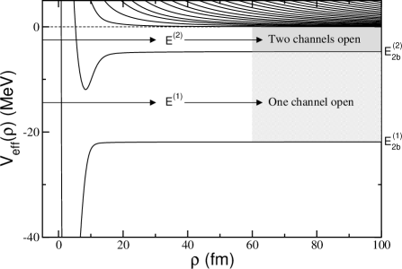
Figure 1: Typical effective adiabatic potentials for a three-body system where two two-body bound states are present. The two lowest adiabatic potentials go asymptotically to the binding energies $E_{2b}^{(1)}$ and $E_{2b}^{(2)}$ of the two-body bound states. For a given three-body energy $E$, when $E_{2b}^{(1)}<E<E_{2b}^{(2)}$ only one channel is open, while when $E_{2b}^{(2)}<E<0$ both channels are open.

A typical behavior of the adiabatic potentials is shown in Fig.1. They correspond to a three-body system where two of the two-body subsystems have a bound state. This is reflected in the fact that the two lowest effective adiabatic potentials go asymptotically to the binding energies $E_{2b}^{(1)}$ and $E_{2b}^{(2)}$ of each bound two-body system. The angular eigenfunctions associated to these two adiabatic potentials have the general asymptotic form nie01 :

$$\Phi_{n}^{JM}(\rho,\Omega)\stackrel{{\scriptstyle\rho\rightarrow\infty}}{{\rightarrow}}\rho^{3/2}\left[\psi_{n}^{j_{x}}(\bm{x})\otimes\left[Y_{\ell_{y}}(\Omega_{y})\otimes\chi_{s_{y}}\right]^{j_{y}}\right]^{JM},$$ (12)

where for this particular case $n=1,2$ and we have now made explicit the quantum numbers. The wave function $\psi_{n}^{j_{x}}(\bm{x})$, normalized to 1 in the $\bm{x}$-Jacobi coordinate, describes the bound two-body system associated to the effective potential $V_{eff}^{(n)}$, whose angular momentum is $j_{x}$. Asymptotically it tends to the bound state wave function of the corresponding two-body subsystem. The spin function $\chi_{s_{y}}$ describes the spin of the third particle, which couples to the orbital angular momentum $\ell_{y}$ (associated to the Jacobi coordinate $\bm{y}$) to give total angular momentum $j_{y}$. Finally, $j_{x}$ and $j_{y}$ couple to the total angular momentum $J$ with projection $M$ of the three-body system.

The analytic form given in Eq.(12) for the asymptotic expression of the angular eigenfunction $\Phi_{n}^{JM}(\Omega,\rho)$ makes evident that it describes an asymptotic spatial distribution for the three particles corresponding to two of them forming a bound state, described by $\psi_{n}^{j_{x}}(\bm{x})$, and a free third particle moving in the continuum. In other words, the effective adiabatic potentials associated to angular eigenfunctions with the asymptotic form of Eq.(12) are the ones describing the possible incoming and outgoing channels of a process where a particle hits a bound state formed by the other two.

In Fig.1 the different regions defined by the energy of the incident particles are depicted. All the three-body energies $E$ such that $E_{2b}^{(1)}<E<E_{2b}^{(2)}$ (like $E^{(1)}$ in the figure) correspond to processes where only one channel is open. Only the elastic collision between the third particle and the bound two-body state with energy $E_{2b}^{(1)}$ is possible. When the three-body energy increases up to the region $E_{2b}^{(2)}<E<0$ ($E^{(2)}$ in the figure) a second channel is open. Two different collisions are now possible, the one where a particle hits the bound state with binding energy $E_{2b}^{(1)}$, and the one where a particle hits the state with binding energy $E_{2b}^{(2)}$. In the same way, each of these reactions has two possible outgoing channels, corresponding to the two allowed bound two-body states and the third particle in the continuum. In particular, in this energy range the rearrangement process is open. When $E>0$ the breakup channels are also open. They are described by the remaining infinitely many adiabatic potentials. Processes with breakup channels open will be investigated in a forthcoming work.

Therefore, for processes where $n_{0}$ channels are open, the full three-body wave function has actually $n_{0}$ different components. We shall denote them by $\Psi_{i}$, corresponding to the process with incident channel $i$. Each of the three-body functions $\Psi_{i}$ is then expanded as in Eq.(4), but the radial functions need now an additional index $i$ ($i\leq n_{0}$) indicating the incident channel to which they correspond:

$$\Psi_{i}=\frac{1}{\rho^{5/2}}\sum_{n=1}^{n_{A}}f_{ni}(\rho)\Phi_{n}(\rho,\Omega).$$ (13)

For each open channel $i$ ($i=1,2,\cdots,n_{0}$) the corresponding radial wave functions $f_{ni}(\rho)$ satisfy the set of radial equations of Eq.(5), and Eq.(9) can be generalized to

$$\left(\begin{array}[]{ccc}\hat{\cal H}_{11}-E&\cdots&\hat{\cal H}_{1n_{A}}\\ \hat{\cal H}_{21}&\cdots&\hat{\cal H}_{2n_{A}}\\ \vdots&\vdots&\vdots\\ \hat{\cal H}_{n_{A}1}&\cdots&\hat{\cal H}_{n_{A}n_{A}}-E\end{array}\right)\left(\begin{array}[]{cccc}f_{11}&f_{12}&\cdots&f_{1n_{0}}\\ f_{21}&f_{22}&\cdots&f_{2n_{0}}\\ \vdots&\vdots&\vdots&\vdots\\ f_{n_{A}1}&f_{n_{A}2}&\cdots&f_{n_{A}n_{0}}\end{array}\right)=0,$$ (14)

which describes the full process. The full three-body wave function is now given by:

$$\Psi=\left(\begin{array}[]{c}\Psi_{1}\\ \Psi_{2}\\ \vdots\\ \Psi_{n_{0}}\end{array}\right)=\frac{1}{\rho^{5/2}}\left(\begin{array}[]{cccc}f_{11}&f_{21}&\cdots&f_{n_{A}1}\\ f_{12}&f_{22}&\cdots&f_{n_{A}2}\\ \vdots&\vdots&\vdots&\vdots\\ f_{1n_{0}}&f_{2n_{0}}&\cdots&f_{n_{A}n_{0}}\end{array}\right)\left(\begin{array}[]{c}\Phi_{1}\\ \Phi_{2}\\ \vdots\\ \Phi_{n_{A}}\end{array}\right)$$ (15)

II.2 Asymptotics: ${\cal K}$-matrix and ${\cal S}$-matrix

For scattering states and energies below the breakup threshold ($E<0$), the Eqs.(14) decouple asymptotically, and for a given incident channel $i$ ($i=1,\cdots,n_{0}$) the only equations surviving are the ones of the form:

$$(\hat{\cal H}_{nn}-E)f_{ni}(\rho)=0\hskip 28.45274pt(n=1,\cdots,n_{A}),$$ (16)

which, by use of Eq.(6), can be written as:

$$\left(-\frac{\hbar^{2}}{2m}\frac{d^{2}}{d\rho^{2}}+V_{eff}^{(n)}(\rho)-E\right)f_{ni}(\rho)=0,$$ (17)

where $V_{eff}^{(n)}$ is given by Eq.(11).

When $n$ corresponds to a closed channel, the radial wave functions $f_{ni}$ vanish asymptotically. When $n$ corresponds to an open channel, the asymptotic behavior of $f_{ni}$ is dictated by the asymptotics of the corresponding adiabatic potential $V_{eff}^{(n)}$. A careful analysis of the large distance behavior of the $\lambda_{n}(\rho)$ and $Q_{nn}(\rho)$ functions in the case of bound two-body subsystems can be found in Ref. nie01 . In particular, Eqs.(91) and (93) of that reference allow to rewrite the above equation for the case $n\leq n_{0}$ as:

$$\left[\frac{d^{2}}{d\rho^{2}}+(k_{y}^{(n)})^{2}-\frac{\ell_{y}(\ell_{y}+1)}{\rho^{2}}\right]f_{ni}(\rho)=0$$ (18)

where

$$k_{y}^{(n)}=\sqrt{\frac{2m}{\hbar^{2}}(E-E_{2b}^{(n)})},$$ (19)

$E_{2b}^{(n)}$ is the binding energy of the bound two-body system associated to the open channel $n$, and $\ell_{y}$ is the orbital angular momentum associated to the Jacobi coordinate $\bm{y}$, which amounts to the relative orbital angular momentum between the projectile and the two-body bound target.

From Eq.(18) it is now clear that the asymptotic behavior of the $f_{ni}$ functions ($n,i\leq n_{0}$) is given by:

$$f_{ni}(\rho)\rightarrow\sqrt{k_{y}^{(n)}}\rho\left(A_{in}^{(K)}j_{\ell_{y}}(k_{y}^{(n)}\rho)+B_{in}^{(K)}\eta_{\ell_{y}}(k_{y}^{(n)}\rho)\right)$$ (20)

where $j_{\ell_{y}}$ and $\eta_{\ell_{y}}$ are the usual regular and irregular spherical Bessel functions, respectively. The superscript $(K)$ indicates that, with this particular choice, the coefficients $A_{in}^{(K)}$ and $B_{in}^{(K)}$ will permit to extract the ${\cal K}$-matrix. Conversely, using the spherical Hankel functions in Eq.(20) the coefficients will form the ${\cal S}$-matrix and the superscript $(S)$ will be used (see below).

Therefore, asymptotically, the matrix containing the radial wave functions in Eq.(15) reduces to the $n_{0}\times n_{0}$ matrix $A^{(K)}J+B^{(K)}Y$, where $A^{(K)}$ and $B^{(K)}$ are $n_{0}\times n_{0}$ matrices whose components are the $A_{ij}^{(K)}$ and $B_{ij}^{(K)}$ coefficients of Eq.(20), and $J$ and $Y$ are two $n_{0}\times n_{0}$ diagonal matrices with diagonal terms $\left(\sqrt{k_{y}^{(i)}}\rho j_{\ell_{y}}(k_{y}^{(i)}\rho)\right)$ and $\left(\sqrt{k_{y}^{(i)}}\rho\eta_{\ell_{y}}(k_{y}^{(i)}\rho)\right)$, respectively. Thus, the asymptotic behavior of the full three-body wave function (15) can be finally written as:

$$\Psi\rightarrow A^{(K)}F_{\rho}^{(K)}+B^{(K)}G_{\rho}^{(K)},$$ (21)

where $F_{\rho}^{(K)}$ and $G_{\rho}^{(K)}$ are column vectors with $n_{0}$ terms of the form $\left(\sqrt{k_{y}^{(n)}}j_{\ell_{y}}(k_{y}^{(n)}\rho)\Phi_{n}/\rho^{3/2}\right)$ and $\left(\sqrt{k_{y}^{(n)}}\eta_{\ell_{y}}(k_{y}^{(n)}\rho)\Phi_{n}/\rho^{3/2}\right)$, respectively.

From Eq.(21) we then have that for a given incident channel $i$ the asymptotic form of the corresponding three-body wave function (13) takes the form:

$$\Psi_{i}\rightarrow\sum_{n=1}^{n_{0}}\left(A_{in}^{(K)}F_{\rho,n}^{(K)}+B_{in}^{(K)}G_{\rho,n}^{(K)}\right)$$ (22)

where

$$F_{\rho,n}^{(K)} \!\!\!\!=\!\!\!\! \sqrt{k_{y}^{(n)}}j_{\ell_{y}}(k_{y}^{(n)}\rho)\left[\psi_{n}^{j_{x}}\otimes\left[Y_{\ell_{y}}(\Omega_{y})\otimes\chi_{s_{y}}\right]^{j_{y}}\right]^{JM}$$

$$G_{\rho,n}^{(K)} \!\!\!\!=\!\!\!\! \sqrt{k_{y}^{(n)}}\eta_{\ell_{y}}(k_{y}^{(n)}\rho)\left[\psi_{n}^{j_{x}}\otimes\left[Y_{\ell_{y}}(\Omega_{y})\otimes\chi_{s_{y}}\right]^{j_{y}}\right]^{JM}$$ (23)

and where we have made use of Eq.(12), which relates the angular eigenfunction $\Phi_{n}^{JM}$ and the two-body wave function $\psi_{n}^{j_{x}}$. When two or three identical particles are present in the system, these functions should be correctly symmetrized or antisymmetrized depending on whether they are either bosons or fermions.

From Eq.(21) we can now easily write:

$$\Psi\rightarrow A^{(K)}\left(F_{\rho}^{(K)}-{\cal K}G_{\rho}^{(K)}\right),$$ (24)

where

$${\cal K}=-{A^{(K)}}^{-1}B^{(K)}$$ (25)

is the ${\cal K}$-matrix of the reaction, whose dimension is $n_{0}\times n_{0}$ (with $n_{0}$ being the number of open channels).

The discussion in this subsection could have also been made by replacing $j_{\ell_{y}}$ and $\eta_{\ell_{y}}$ in Eq.(20) by the spherical Hankel functions $h_{\ell_{y}}^{(2)}$ and $h_{\ell_{y}}^{(1)}$, respectively. This would then lead to:

$$\Psi\rightarrow A^{(S)}F_{\rho}^{(S)}+B^{(S)}G_{\rho}^{(S)},$$ (26)

where now $F_{\rho}^{(S)}$ and $G_{\rho}^{(S)}$ are column vectors with $n_{0}$ terms of the form $\left(\sqrt{k_{y}^{(n)}}h_{\ell_{y}}^{(2)}(k_{y}^{(n)}\rho)\Phi_{n}/\rho^{3/2}\right)$ and $\left(\sqrt{k_{y}^{(n)}}h_{\ell_{y}}^{(1)}(k_{y}^{(n)}\rho)\Phi_{n}/\rho^{3/2}\right)$, respectively. We can then write:

$$\Psi\rightarrow A^{(S)}\left(F_{\rho}^{(S)}+{\cal S}G_{\rho}^{(S)}\right),$$ (27)

where

$${\cal S}={A^{(S)}}^{-1}B^{(S)}$$ (28)

is the so called ${\cal S}$-matrix of the reaction. The ${\cal S}$ and ${\cal K}$ matrices are related through the well known simple expression:

$${\cal S}=(1+i{\cal K})(1-i{\cal K})^{-1}.$$ (29)

It is important to keep in mind that while $A^{(K)}$, $B^{(K)}$, and ${\cal K}$ are real, the matrices $A^{(S)}$, $B^{(S)}$, and ${\cal S}$ are in general complex.

III Second order integral relations

In Ref.bar09 the applicability of the HA expansion to extract phase shifts for 1+2 reactions when only the elastic channel is open has been discussed. In that reference it was found that, when increasing the number of adiabatic channels $n_{A}$ included in the calculation as much as possible, the difference between the computed phase shift and the exact value remains significant. As mentioned in the Introduction, this is related to the fact that the asymptotic structure of the system has to be describe in terms of spherical Bessel functions depending on $k_{y}y$, where $y$ is the modulus of the Jacobi coordinate between the center of mass of the outgoing bound two-body system and the third particle. Instead, the asymptotic behavior using the HA basis is given in terms of spherical Bessel functions depending on $k_{y}\rho$. Since the equivalence between $k_{y}y$ and $k_{y}\rho$ is not matched for any finite value of $\rho$, the correct boundary condition is only achieved at $\rho\approx\infty$ and $n_{A}\rightarrow\infty$.

For a general multichannel process the adiabatic expansion obviously shows the same deficiency. The correct asymptotic wave function is given by Eq.(21), but where $F_{\rho}^{(K)}$ and $G_{\rho}^{(K)}$ in Eq.(23) have to be replaced by $F^{(K)}$ and $G^{(K)}$, which are column vectors whose $n$-th element is

$$F_{n}^{(K)} \!\!\!\!=\!\!\!\! \sqrt{k_{y}^{(n)}}j_{\ell_{y}}(k_{y}^{(n)}y_{n})\left[\psi_{n}^{j_{x}}\otimes\left[Y_{\ell_{y}}(\Omega_{y})\otimes\chi_{s_{y}}\right]^{j_{y}}\right]^{JM}$$

$$G_{n}^{(K)} \!\!\!\!=\!\!\!\! \sqrt{k_{y}^{(n)}}\eta_{\ell_{y}}(k_{y}^{(n)}y_{n})\left[\psi_{n}^{j_{x}}\otimes\left[Y_{\ell_{y}}(\Omega_{y})\otimes\chi_{s_{y}}\right]^{j_{y}}\right]^{JM}.$$ (30)

In these expressions $y_{n}$ refers to the modulus of the Jacobi coordinate describing the center of mass of the bound two-body system $\psi_{n}^{j_{x}}$ and the third particle.

It is important to recall that the Bessel functions $\eta_{\ell}$ are irregular at the origin, which creates difficulties from the numerical point of view. It is then convenient to regularize such function, in such a way that $G_{n}^{(K)}$ given in Eq.(30) has to be replaced by:

$$\widetilde{G}_{n}^{(K)}=\left(1-e^{-\gamma y_{n}}\right)^{\ell_{y}+1}G_{n}^{(K)}$$ (31)

where $\gamma$ is a non linear parameter. The results are stable for values of $\gamma$ within a small range around $\gamma\sim 1/r_{0}$, with $r_{0}$ the range of the potential.

For simplicity in the notation, from now on, we shall refer to the matrices $\{F^{(K)},\widetilde{G}^{(K)}\}$ as $\{F,G\}$, in such a way that we can write the asymptotic behavior of the wave function as:

$$\Psi\rightarrow AF+BG,$$ (32)

and ${\cal K}=-A^{-1}B$.

The vectors $F$ and $G$ satisfy the following normalization condition:

$$-\frac{2m}{\hbar^{2}}\left[\langle F|\hat{\cal H}-E|G\rangle-\langle G|\hat{\cal H}-E|F\rangle^{T}\right]=\mathbbm{I}.$$ (33)

where $\mathbbm{I}$ is the identity matrix. In Eq.(33) we have introduced a notation to be used from now on in which the overlap of two vectors is a matrix whose elements are, for example, $(\langle F|\hat{\cal H}-E|G\rangle)_{ij}=\langle F_{i}|\hat{\cal H}-E|G_{j}\rangle$. The normalization condition allows to extract a first order estimate of the matrices $A$ and $B$ from the scattering wave function $\Psi$ as

$$B^{1^{st}} = -\frac{2m}{\hbar^{2}}\left[\langle F|\hat{\cal H}-E|\Psi\rangle^{T}-\langle\Psi|\hat{\cal H}-E|F\rangle\right]$$ (34)

$$A^{1^{st}} = -\frac{2m}{\hbar^{2}}\left[\langle\Psi|\hat{\cal H}-E|G\rangle-\langle G|\hat{\cal H}-E|\Psi\rangle^{T}\right].$$ (35)

Clearly, when $\Psi$ is an exact solution of $(\hat{\cal H}-E)\Psi=0$, the above expressions reduce to the the following integral relations:

$$B = \frac{2m}{\hbar^{2}}\langle\Psi|\hat{\cal H}-E|F\rangle$$

$$A = -\frac{2m}{\hbar^{2}}\langle\Psi|\hat{\cal H}-E|G\rangle.$$ (36)

Explicitly, each matrix element $B_{ij}$ and $A_{ij}$ is given by:

$$B_{ij} = \frac{2m}{\hbar^{2}}\langle\Psi_{i}|\hat{\cal H}-E|F_{j}\rangle$$ (37)

$$A_{ij} = -\frac{2m}{\hbar^{2}}\langle\Psi_{i}|\hat{\cal H}-E|G_{j}\rangle,$$ (38)

which can be seen as the extension to multichannel scattering of the expressions valid for the single channel case. Now the same formula applies for each possible incoming channel described by $\Psi_{i}$ and each possible outgoing channel whose asymptotic analytic form is given by a linear combination of $F_{j}$ and $G_{j}$.

As demonstrated in Refs. bar09 ; kiev10 for a single channel process, the relation ${\cal K}=-A^{-1}B$ computed using Eqs.(37) and (38) can be considered accurate up to second order when a trial wave function $\Psi_{t}$ is used. Moreover the two integral relations of Eqs.(37) and (38) can be directly derived from the Kohn Variational Principle. As shown in Appendix A, the matrix form of of KVP, necessary to describe a multichannel process, establishes that each matrix element of $A^{-1}B^{2^{nd}}$ is a functional given by

$$A^{-1}B^{2^{nd}}=A^{-1}B+\frac{2m}{\hbar^{2}}A^{-1}\langle\Psi_{t}|\hat{\cal H}-E|\Psi_{t}\rangle(A^{-1})^{T}\;,$$ (39)

which is stationary with respect to variations of the wave function. Taking into account the general asymptotic behavior in Eq.(32), we can write the full trial wave function schematically as:

$$\Psi_{t}=\Psi_{c}+AF+BG,$$ (40)

with $\Psi_{c}\rightarrow 0$ as $\rho\rightarrow\infty$. Furthermore $\Psi_{c}$ can be expanded in terms of a (square integrable) complete basis $\{b_{i},i=1,\cdots,m\}$:

$$\Psi_{c}=\left(\begin{array}[]{c}\Psi_{c,1}\\ \Psi_{c,2}\\ \vdots\\ \Psi_{c,n_{0}}\end{array}\right)=\frac{1}{\rho^{5/2}}\left(\begin{array}[]{cccc}c_{11}&c_{12}&\cdots&c_{1m}\\ c_{21}&c_{22}&\cdots&c_{2m}\\ \vdots&\vdots&\vdots&\vdots\\ c_{n_{0}1}&c_{n_{0}2}&\cdots&c_{n_{0}m}\end{array}\right)\left(\begin{array}[]{c}b_{1}\\ b_{2}\\ \vdots\\ b_{m}\end{array}\right),$$ (41)

The variation of the functional with respect to the linear parameters $c_{ij}$ and with respect to the matrix elements of $A^{-1}B$ leads to:

$$\langle\Psi_{c}|\hat{\cal H}-E|\Psi_{t}\rangle = 0$$

$$\langle G|\hat{\cal H}-E|\Psi_{t}\rangle = 0$$ (42)

When $\Psi$ is replaced by $\Psi_{t}$, the second expression above and Eq.(35) result:

$$A=-\frac{2m}{\hbar^{2}}\langle\Psi_{t}|\hat{\cal H}-E|G\rangle.$$ (43)

Replacing now Eq.(40) into (39), and making use of the Eqs.(42), we also get:

$$B^{2^{nd}}=B^{1^{st}}+\frac{2m}{\hbar^{2}}\langle F|\hat{\cal H}-E|\Psi_{t}\rangle^{T},$$ (44)

and, taking into account that $B^{1^{st}}$ is given by Eq.(34) we can then obtain the final result:

$$B^{2^{nd}} = \frac{2m}{\hbar^{2}}\langle\Psi_{t}|\hat{\cal H}-E|F\rangle$$

$$A = -\frac{2m}{\hbar^{2}}\langle\Psi_{t}|\hat{\cal H}-E|G\rangle,$$ (45)

which according to Eqs.(25) and (29) permit to obtain the second order estimate of the ${\cal K}$-matrix or the ${\cal S}$-matrix, ${\cal K}^{2^{nd}}$ or ${\cal S}^{2^{nd}}$, respectively.

In practical cases, application of the integral relations given in Eq.(45) require the calculation of each individual matrix element $A_{ij}$ and $B_{ij}$, which relate each possible incoming channel $i$ described by $\Psi_{i}$, with each possible outgoing asymptotics given by $F_{j}$ and $G_{j}$. Details about the calculation of these matrix elements are given in appendix B, in particular for the case of two-body potentials projecting on the partial waves.

The integral relations of Eq.(45) depend on the short range structure of the scattering wave function $\Psi_{t}$ as $F$ and $G$ are asymptotically solutions of $({\cal H}-E)F,G=0$. This property allows for different applications of the integral relations, as discussed in Ref. kiev10 . In the present work the interest is given in the study of the pattern of convergence of ${\cal K}^{2^{nd}}$ in terms of the number of equations $n_{A}$ considered in the description of $\Psi_{t}$ using the HA expansion. As we will see, increasing $n_{A}$, both matrices $A$ and $B^{2^{nd}}$ slightly change, showing individually a very slow rate of convergence. Conversely, its rate ${\cal K}^{2^{nd}}=-A^{-1}B^{2^{nd}}$ shows a pattern of convergence similar to that one observed in a bound state calculation.

IV Results

IV.1 Test of the method: A model 1+2 collision

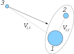
Figure 2: Scheme of the model reaction used to test the integral relations. The light projectile 3 hits the dimer made by particles 1 and 2. Particle 1 is infinitely heavy and particles 2 and 3 do not interact.

To test the method we have chosen a 1+2 reaction where the target dimer is made by an infinitely heavy particle and a light one, and where we consider a projectile interacting only with the heavy particle (see Fig.2). In the collision particle 2 does not play any role, and the process is equivalent to a two-body reaction between particles 3 and 1. Therefore the results obtained through the three-body calculation and the integral relations can be easily tested by means of a simple two-body calculation.

In particular, we consider a two-body target made by two spin-zero bosons with masses $0.5m$ and $10^{12}m$ (with $m=938.69461$ MeV) interacting via a simple central potential given by

$$V_{12}(r)=-80\;e^{-r^{2}/1.6^{3}}$$ (46)

where $r$ is given in fm and the strength in MeV. This system has only one $s$-wave bound state with binding energy $-6.2757$ MeV.

The projectile, which is chosen to have a mass of $0.51m$, does not interact with particle 2, while it does it with particle 1 through the gaussian potential:

$$V_{13}(r)=-30\;e^{-r^{2}/1.6^{2}},$$ (47)

where again $r$ is in fm and the strength in MeV. This potential is not able to bind particles 1 and 3. Finally, as described above, $V_{23}=0$.

We have chosen an incident energy of $3$ MeV, which implies a total three-body energy of $-3.2757$ MeV. We are then below the threshold for breakup of the two-body target, and only the elastic channel is open. Therefore, $B$ and $A$ in Eq.(45) are just numbers, and they are such that $\tan\delta_{\ell}=-B/A$ (note that the definition of $B$ in here and in bar09 ; kiev10 have opposite sign).

Table 1: Partial wave phase shifts $\delta_{\ell}$ for different values of $n_{A}$ (number of adiabatic terms used in the expansion (4)). In the last row, the result using a two-body calculation is shown.

$n_{A}$	$\delta_{s}$	$\delta_{p}$	$\delta_{d}$
1	40.554	0.6658	0.0136
2	38.988	0.6892	0.0113
3	38.642	0.6921	0.0121
5	38.693	0.6911	0.0119
8	38.702	0.6918	0.0118
10	38.701	0.6918	0.0118
two-body	38.699	0.6917	0.0117

We have computed the phase shift for this reaction for relative $s$, $p$, and $d$ waves between the projectile and the target. The convergence of the expansion (4) is shown in table 1, where we show the phase shift for the different partial waves and for different values of $n_{A}$, which is the number of adiabatic terms included in the calculation. As we can see, inclusion of 8 to 10 adiabatic potentials is enough to reach convergence for the three partial waves. Furthermore, the converged result agrees with the phase shift obtained from the two-body calculation describing the collision between particles 3 and 1.

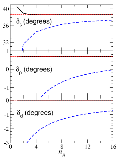
Figure 3: (color online) Phase-shift for $s$, $p$, and $d$ partial waves for the model reaction in section  IV.1 as a function of the number of adiabatic terms included in the calculation. The solid line is the result obtained through the integral relations, and the thick dashed curve has been obtained from the asymptotic expression (20). The thin dashed line is the result obtained from a two-body calculation.

The efficiency of using the integral relations in Eq.(45) is made evident in Fig. 3, where we show the partial wave phase shifts $\delta_{\ell}$ as a function of $n_{A}$. The solid line gives the results obtained from the integral relations (given in table 1), and the thick dashed line shows the results extracted by direct comparison of the computed asymptotic radial wave functions and the analytic expression in Eq. (20). The thin dashed line indicates the phase shifts obtained from a two-body calculation. As we can immediately see in the figure, the pattern of convergence of the phase shifts obtained from Eq.(20) (thick dashed curves) is very slow. A simple extrapolation of these curves up to the correct value permits to foresee that the number of adiabatic terms needed to obtain accurate values of $\delta_{\ell}$ is far larger than the one needed when the integral relations are used. In fact, at the scale of the figure, the calculations with the integral relations are already for $n_{A}=4$ indistinguishable from the correct result (see also table 1).

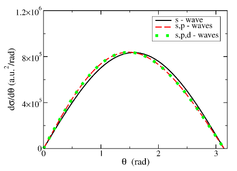
Figure 4: (color online) Cumulative contributions to the differential cross section as a function of the scattering angle $\theta$ for the model collision in section IV.1.

As seen in table 1, the $d$-wave phase shift is already rather small and therefore, at the considered energy, the cross section contributions from higher angular partial waves is negligible. In Fig. 4 the differential cross section of the process with cumulative inclusion of one (solid), two (dashed), and three (dot-dashed) partial waves is shown. As can be seen, $s$-, $p$ and $d$-partial waves are enough to obtain a converged cross section of the process. In fact, the partial waves beyond the $s$-wave have a modest contribution, and the total cross section approaches quite a lot the characteristic $\sin\theta$ function of the $s$-waves.

IV.2 A realistic case: The ⁴He -⁴He₂ collision

In this section we discuss an interesting simple physical case, but technically similar to the model case described in the previous section. This is the collision of a ⁴He atom into the weakly bound ⁴He₂ dimer. The helium dimer has a single $s$-wave bound state, and as soon as the incident energy is below the dimer breakup threshold, again only the elastic channel is open.

The two-body helium-helium interaction is chosen to be the simple effective gaussian potential given in nil98 . This is enough for our purpose of illustrating how this kind of processes can be easily described by use of the integral relations. This potential is built to reproduce the $s$-wave scattering length (189.054 a.u.) and effective range (13.843 a.u.) of the LM2M2 interaction azi91 , and it is given by:

$$V_{2B}(r)=-1.227\;e^{-r^{2}/10.03^{2}}$$ (48)

where $r$ is given in a.u. and the strength is in K. This potential leads to a bound 0^{+ 4}He₂ dimer with a binding energy $E_{d}=-1.2959$ mK, a scattering length $a=189.947$ a.u., and an effective range of 13.846 a.u.. Simple representations of the atom-atom potentials are often used to describe reactions in the ultracold regime (see for example Refs. incao08 ; stecher09 ). In this regime the process is largely independent of the shape of the potential and can be characterized only by the scattering length.

With this interaction the helium trimer has two bound states at $-150.0$ mK and $-2.467$ mK. These states have been obtained using the gaussian potential active only in $s$-waves. Increasing the number of partial waves up to $\ell_{x}=\ell_{y}=8$ results in a very small change for the ground and excited state binding energies, which become now $150.4$ mK and $-2.472$ mK, respectively. In fact, more than 99% of the norm of the bound state wave functions is provided by the lowest adiabatic term, whose corresponding adiabatic potential is close to identical in both calculations. Accordingly, in the following we restrict the calculations to include only the $\ell_{x}=0$ channel.

When the LM2M2 potential is used, these two states are found to have binding energies $-126.4$ mK and $-2.265$ mK, respectively bar01 . As we can see, the ground state is not very well reproduced when the gaussian version of the potential is used. In this very deep state, the three atoms are close to each other and the correct structure can not be described with the simplified potential. Conversely, the excited state which has the characteristic of an Efimov state has an structure in which the third atom orbits very far from the bound state of the other two. This particular structure is well described by the attractive gaussian potential.

Table 2: Partial wave phase shifts $\delta_{\ell}$ are given showing convergence of these values with the number $n_{A}$ of adiabatic potential used in the calculation. The last row shows the result when the Hyperspherical Harmonic method kiev08 is used.

$n_{A}$	$\delta_{s}$	$\delta_{p}$	$\delta_{d}$	$\delta_{f}$
1	-39.72	-13.19	2.01	-0.27
2	-40.30	-13.13	2.11	-0.28
4	-40.43	-13.11	2.13	-0.28
8	-40.50	-13.11	2.14	-0.28
18	-40.54	-13.11	2.14	-0.28
22	-40.54	-13.11	2.14	-0.28
HH-calculation	-40.55	—	—	—

In order to study the convergence properties of the HA expansion for a $1+2$ collision, we have chosen an incident energy of $0.5$ mK (or a three-body energy $E=-0.7959$ mK). The phase shifts for the different partial waves have been computed as in the previous subsection. The results are shown in table 2 for $s$, $p$, $d$, and $f$ waves. A good convergence is obtained already after inclusion of about 10 adiabatic terms, except for $s$-waves, where about 18 are needed. The last row in the table shows the phase shift obtained for an $s$-wave collision when the Hyperspherical Harmonic method is used. The two methods are in close agreement.

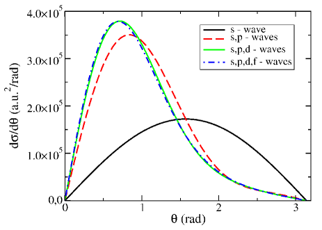
Figure 5: (color online) The same as in Fig.4 for the ⁴He -⁴He₂ collision. With four partial waves the convergence is fairly good.

At this particular energy we have calculated the differential cross section. Fig. 5 shows the cumulative contributions of the $s$, $p$, $d$ and $f$ partial waves. We observe that the $p$-wave contribution is rather important and produces a deviation from the $\sin\theta$ shape. Moreover, four partial waves are needed to reach a good convergence.

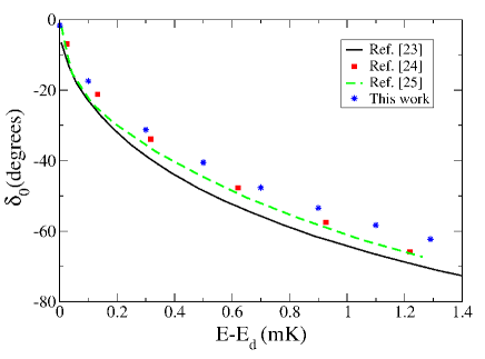
Figure 6: (color online)$s$-wave phase shift $\delta_{s}$ as a function of the incident energy for the ⁴He -⁴He₂ collision. The stars are the results obtained in the present work. The solid curve, the squares, and dashed curve correspond to the results given in sun08 , rou03 , and mot01 , respectively.

In Fig. 6 we show the computed $s$-wave phase shift as a function of the incident energy ($E-E_{d}$). Our results are given by the stars. For comparison we also show the results reported in sun08 , rou03 , and mot01 (solid curve, squares, and dashed curve, respectively). As we can see, the phase shifts obtained in this work are a few degrees above the ones obtained in the previous calculations, where the ⁴He -⁴He interaction is treated more in detail. In fact the reason for this discrepancy is the hard core repulsion present in the ⁴He -⁴He interactions used in sun08 ; rou03 ; mot01 . For the same reason the atom-dimer scattering length $a_{a-d}$ obtained with the gaussian potential used in this work, $a_{a-d}=166$ a.u., differs from the typical values of around $a_{a-d}=220$ a.u. ($\approx 116$ Å) obtained when hard core potentials are used rou03 ; kol04 .

IV.3 A multichannel collision: The ⁴He-⁴He-⁶Li system

In this subsection a reaction where more than one channel is open is discussed. To this aim, we have chosen a process involving two helium and one lithium atoms. The cross section for this kind of reactions is the necessary ingredient to obtain the recombination rate for such three-body systems. As quoted in suno09 , where the three-body recombination for cold helium-helium-alkali-metal systems is investigated, such collision processes are important in ultracold gas experiments using buffer-gas cooling, since it might limit the lifetimes of the trapped atoms.

To describe this three-body system we take the same helium-helium interaction as in the previous section, which leads to a 0^{+ 4}He₂ dimer with a binding energy of $-1.2959$ mK. The lithium-helium interaction is also chosen to have a gaussian shape, and it is taken to be:

$$V_{(^{6}{\rm Li}-^{4}{\rm He})}(r)=-0.27368\;e^{-r^{2}/20.14^{2}},$$ (49)

where $r$ is in a.u. and the strength is in K. The parameters have been adjusted to give a scattering length of $-173.5$ a.u. and an effective range of $26.475$ a.u. in agreement with the values obtained in kle99 ($a=-173.8$ a.u. and $r_{e}$=26.483 a.u.), where the more sophisticated KTTY potential is used. This potential leads to a 0⁺ bound ⁶Li-⁴He system with a binding energy of $-1.4225$ mK.

The adiabatic potentials obtained for the ⁴He-⁴He-⁶Li three-body system follow the same pattern as the potentials in Fig.1, where $E_{2b}^{(1)}$ corresponds now to the binding energy of the ⁶Li-⁴He dimer ($-1.4225$ mK) and $E_{2b}^{(2)}$ corresponds to the binding energy of the ⁴He₂ dimer ($-1.2959$ mK). The three-body system presents one bound state at $E=-58.12$ mK.

Thus, as soon as the three-body energy lies in the same region as $E^{(2)}$ in the figure, two different channels are open. One of them corresponds to a bound ⁶Li-⁴He dimer and the second ⁴He atom in the continuum (we shall refer to it as channel 1), and the other one corresponds to the bound ⁴He₂ dimer and the ⁶Li atom in the continuum (we shall refer to it as channel 2). In other words, when taking channel 1 as the incoming channel we are considering a process were the ⁴He atom hits a bound ⁶Li-⁴He dimer, while when choosing channel 2 as the incoming channel we are then considering the process of a ⁶Li atom hitting a ⁴He₂ dimer. For each of the two possible incoming channels we have two different outgoing channels, the elastic one and a rearrangement process where the projectile is captured by one of the constituents of the dimer, while the second dimer constituent is released.

The existence of two open channels implies that the ${\cal K}$-matrix (or the ${\cal S}$-matrix) is a 2$\times$2 matrix, that can be obtained through the 2$\times$2 matrices $A$ and $B^{2^{nd}}$ in Eq.(45). Each of the four terms in $A$ and $B^{2^{nd}}$ can be obtained as in Eqs.(38) and (37) where $\Psi_{i}$ is the trial three-body wave function for the incoming channel $i$. $F_{j}$ and $G_{j}$ are the asymptotic functions given in Eqs.(30) for the outgoing channel $j$. These functions have to be symmetrized when the outgoing channel is 1, since the helium atom in the dimer is identical to the one moving in the continuum. For outgoing channel 2 this is not necessary, since the dimer wave function in (30) is already properly symmetrized. In practice, the symmetrization gives out a factor of $\sqrt{2}$ in Eqs.(37) and (38) when $j$=1. The calculation of each of these terms is formally identical to the case with only the elastic channel open.

Table 3: ${\cal K}$-matrix elements are given as a function of the number of adiabatic potentials used in the calculation ($n_{A}$).

$n_{A}$	${\cal K}_{11}$	${\cal K}_{12}$	${\cal K}_{21}$	${\cal K}_{22}$
2	-2.460	-0.650	-0.648	-1.411
3	-2.765	-0.821	-0.801	-1.496
4	-2.691	-0.775	-0.776	-1.468
6	-2.699	-0.781	-0.781	-1.471
8	-2.702	-0.783	-0.783	-1.471
10	-2.710	-0.787	-0.787	-1.473
14	-2.714	-0.790	-0.789	-1.474
18	-2.712	-0.791	-0.790	-1.474

In the calculation here we have chosen a three-body energy of $-0.7959$ mK, which represents an incident energy of $0.6266$ mK when channel 1 is the incoming channel, and $0.5$ mK when channel 2 is the incoming channel. For simplicity we restrict in this section to relative $s$-waves between the projectile and the dimer target. The computed result for the four terms of the ${\cal K}$-matrix are shown in table 3 for different values of $n_{A}$. As seen in the table, again a reduced amount of adiabatic terms permits to reach a reasonable convergence in the ${\cal K}$-matrix.

From the computed ${\cal K}$-matrix we can now easily obtain the ${\cal S}$-matrix by means of Eq.(29). This leads to ${\cal S}_{11}=-0.673-0.663i$, ${\cal S}_{12}={\cal S}_{21}=-0.285+0.162i$, and ${\cal S}_{22}=-0.224-0.918i$. The square of these elements, $|{\cal S}_{ij}|^{2}$, indicates the probability for the process with incoming channel $i$ to end up in channel $j$. In this particular case we get $|S_{11}|^{2}=|S_{22}|^{2}=0.892$ and $|S_{12}|^{2}=|S_{21}|^{2}=0.108$.

It is important to note that the matrices $A$ and $B^{2^{nd}}$ are not unique. A different definition of the normalization of the asymptotic states would result into new $A$ and $B^{2^{nd}}$ matrices which would obviously lead to the same ${\cal K}$-matrix. In particular, $A$ and $B^{2^{nd}}$ do not fulfill the property of being symmetric, but they lead to a ${\cal K}$-matrix with the correct hermitian condition. Moreover, using Eq.(29), the computed ${\cal S}$-matrix automatically satisfies the unitarity condition ${\cal S}^{\dagger}{\cal S}=\mathbbm{I}$.

V Summary and conclusions

In this work we have discussed the general form of the integral relations that were introduced in bar09 ; kiev10 . These relations are derived from the Kohn Variational Principle and they permit to exploit the particularities of the adiabatic expansion method to describe scattering states. In particular, in bar09 ; kiev10 it was shown that the convergence of the computed scattering phase shifts in terms of the adiabatic terms included in the calculation is rather fast. The convergence pattern results to be similar to the one of a bound state calculation. The reason for this success is that when using the integral relations only the internal part of the wave function is needed, and an accurate calculation of it requires a smaller amount of adiabatic terms than when computing the wave function in the asymptotic region.

The applications given in bar09 ; kiev10 were limited to processes involving only relative $s$-waves and with only one channel open. In this work we have explicitly derived the integral relations from the KVP in the case of multichannel reactions and we have computed phase-shifts up to $f$-waves. Furthermore, we have used a vectorial notation for the wave function such that all the possible channels are simultaneously represented. With this notation the coefficients weighting the regular and irregular part of the asymptotic wave function are $n_{0}\times n_{0}$ matrices (with $n_{0}$ being the number of open channels) and each term of these two matrices is obtained from an integral relation. Finally, the ${\cal K}$-matrix for a given process is obtained as the product of two $n_{0}\times n_{0}$ matrices.

Although the method derived is completely general, in this work we have restricted ourselves to describe $1+2$ reactions with projectile energy below the breakup threshold in three outgoing particles. Therefore, only elastic, inelastic, and rearrangement processes are possible.

To test the method when including relatives partial waves higher than zero, we have first used a toy model such that the three-body reaction is fully equivalent to a two-body process. In this way the correct phase shift can be easily computed through a simple two-body calculation. We have found a slow convergence of the phase shifts when extracted from the asymptotic part of the radial wave functions. Conversely, the rate $A^{-1}B$ converges much faster and the result stabilize with a rather small number of adiabatic channels. The convergence is equally fast for all the partial waves, and around 10 adiabatic terms are enough to reach a good convergence. Furthermore, the phase shifts obtained with the two-body calculations are well reproduced.

As the next step, we have analyzed a more physical case, in particular the ⁴He -⁴He₂ collision. Since we have considered energies below the ⁴He₂ breakup threshold, in this reaction only the elastic channel is open. This is a process technically analogous to the previous schematic case for which the method has been proved to work. In fact, a similar pattern of convergence is found for the different partial waves included in the calculation. Inclusion of partial waves with $\ell$ up to 3 are needed to obtain a converged cross section for the process. For $s$-waves the computed phase shift reproduces the one obtained with the Hyperspherical Harmonic expansion method.

Finally, we have considered a process with two open channels. We have chosen a three-body system made by two ⁴He and one ⁶Li atoms, where two different dimers, ⁴He₂ and ⁴He -⁶Li, are possible. We have therefore simultaneously investigated the collision between a ⁴He atom and a ⁴He -⁶Li dimer, and the one between a ⁶Li atom and a ⁴He₂ dimer. For both reactions two possible outgoing channels (elastic and rearrangement) are permitted. We have then used the method to obtain the $2\times 2$ ${\cal K}$-matrix. Again, we have found a fast convergence of the four terms in ${\cal K}$. Furthermore, the computed ${\cal K}$-matrix satisfies the required hermitian condition, as well as the fact of leading to a unitary ${\cal S}$-matrix.

Summarizing, we have shown that the integral relations can be easily applied to reactions involving non-zero partial waves and with more then one channel open. Also in this case, the hyperspherical adiabatic expansion method is a highly efficient tool that permits to obtain scattering wave functions. The ${\cal K}$-matrix, and therefore also the ${\cal S}$-matrix, converges rather fast. Also, since the hyperspherical adiabatic expansion method permits to identify every single incoming and outgoing open channel with a single adiabatic term, the dimension of the matrices to be computed is rather modest, typically of the same size as the number of open channels in the reaction.

Appendix A Matrix form of the Kohn Variational Principle

This derivation is completely analogous to the derivation presented in Ref. koh48 . The only difference is that, in order to represent each possible incoming channel, we use the vectorial notation for the wave functions as introduced in the present work, where the total wave function $\Psi$ has the form given in Eq.(15).

We start by taking the matrix given by:

$$I\equiv\langle\Psi|\hat{\cal H}-E|\Psi\rangle$$ (50)

which vanishes when $\Psi$ is the exact wave function. We then introduce a test wave function $\Psi_{t}=\Psi+\delta\Psi$ so that its radial wave functions verify:

$$f_{ni}^{t}(0)=0$$ (51)

$$f_{ni}^{t}(\rho\to\infty)\rightarrow\sqrt{k_{y}^{(n)}}\rho\left(A_{in}j_{\ell_{y}}(k_{y}^{(n)}\rho)+B^{t}_{in}\eta_{\ell_{y}}(k_{y}^{(n)}\rho)\right).$$

We can then write $f_{ni}^{t}=f_{ni}+\delta f_{ni}$, where $\delta f_{ni}$ satisfies that

$$\delta f_{ni}(\rho)\to\sqrt{k_{y}^{(n)}}\rho\;\eta_{\ell_{y}}(k_{y}^{(n)}\rho)\;\delta B_{in}.$$ (52)

The matrix in Eq.(50), evaluated at the test wave function, is:

$$I_{t}=\delta I=\langle\Psi_{t}|\hat{\cal H}-E|\Psi_{t}\rangle$$ (53)

Using now that the exact wave function verifies that $(\hat{\cal H}-E)|\Psi\rangle=0$, and keeping only the first order terms, the matrix above can be written as:

$$\delta I=\langle\Psi|\hat{\cal H}-E|\delta\Psi\rangle-\langle\delta\Psi|\hat{\cal H}-E|\Psi\rangle^{T}$$ (54)

Using the expansion of $\Psi$ given in Eq. (13) and the analytical expression of the operator $\hat{\cal H}$ from Eq. (2), it can be seen that each matrix element of $\delta I$ takes the form:

$$\delta I_{ij} = \frac{\hbar^{2}}{2m}\sum_{n}\int_{0}^{\infty}d\rho\frac{d}{d\rho}\left(\frac{df_{ni}}{d\rho}\delta f_{nj}-\frac{d(\delta f_{nj})}{d\rho}f_{ni}\right)$$ (55)

$$- \frac{\hbar^{2}}{m}\sum_{n}\int_{0}^{\infty}d\rho\frac{d}{d\rho}\left(P_{ij}(\rho)f_{ni}\delta f_{nj}\right),$$

where $P_{ij}(\rho)$ are the coupling terms appearing in Eq. (7), and given in Eq.(8), which vanish when $\rho$ tends to zero or to infinity. Therefore the last term in the previous expression vanishes, and, since $f_{ni}(0)=0$, we get:

$$\delta I_{ij}=\frac{\hbar^{2}}{2m}\sum_{n}\left[\frac{df_{ni}}{d\rho}\delta f_{nj}-\frac{d(\delta f_{nj})}{d\rho}f_{ni}\right]_{\rho=\infty}$$ (56)

which, using Eq.(20) and Eq.(52), leads to:

$$\delta I_{ij}=-\frac{\hbar^{2}}{2m}\sum_{n}A_{in}\delta B_{jn}=-\frac{\hbar^{2}}{2m}\left\{A\delta B^{T}\right\}_{ij},$$ (57)

or, in a more compact way:

$$\delta\left(I+\frac{\hbar^{2}}{2m}AB^{T}\right)=0.$$ (58)

Since for the exact wave function $\Psi$ we have that $I=0$, we finally get:

$$\frac{\hbar^{2}}{2m}AB^{T}=I_{t}+\frac{\hbar^{2}}{2m}AB^{T}_{t},$$ (59)

which becomes a variational principle for $AB^{T}$. Therefore, given a test wave function $\Psi_{t}$, we obtain a second order correction for $AB^{T}$ as:

$$A(B^{2^{nd}})^{T}=AB^{T}+\frac{2m}{\hbar^{2}}\langle\Psi_{t}|\hat{\cal H}-E|\Psi_{t}\rangle$$ (60)

If we now multiply from the left by $A^{-1}$ and from the right by $(A^{-1})^{T}$, and make use of the fact that the ${\cal K}$-matrix is symmetric, i.e. $A^{-1}B=B^{T}(A^{-1})^{T}$, we then finally get the expression given in Eq.(39).

Appendix B Calculation of the integrals in $A$ and $B$

In this appendix we give details of the calculation of the integrals $A$ and $B$, in particular when using two-body potentials projecting on partial waves. To this aim let us start from the general expression for $A$ and $B$ in Eq.(45), and write the ${\cal L}$ operator in its explicit form

$${\cal L}=\frac{2m}{\hbar^{2}}(\hat{{\cal H}}-E)=\frac{2m}{\hbar^{2}}\Big{(}-\frac{\hbar^{2}}{2m}\bigtriangledown^{2}_{\bm{y_{1}}}$$ (61)

$$-\frac{\hbar^{2}}{2m}\bigtriangledown^{2}_{\bm{x_{1}}}+\hat{V}_{1}(x_{1})+\hat{V}_{2}(x_{2})+\hat{V}_{3}(x_{3})-E_{d}-E_{0}\Big{)}$$

where $E_{d}$ is the binding energy of the dimer and $E_{0}$ is the incident energy of the projectile. The Jacobi coordinates $(\bm{x}_{1},\bm{y}_{1})$ are defined such that $\bm{x}_{1}$ connects the two particles in the dimer (particles 2 and 3). The coordinates $x_{2}$ and $x_{3}$ are related to the distances between particles 1 and 3, and between particles 1 and 2, respectively.

Using $F$ and $G$ as defined in (30) we can rewrite Eq.(45) as:

$$B^{2^{nd}} = \frac{2m}{\hbar^{2}}<\Psi|\hat{V}_{2}(x_{2})+\hat{V}_{3}(x_{3})|F(\bm{x}_{1},\bm{y}_{1})>$$ (62)

$$A = -\frac{2m}{\hbar^{2}}<\Psi|\hat{V}_{2}(x_{2})+\hat{V}_{3}(x_{3})|{\widetilde{G}}(\bm{x}_{1},\bm{y}_{1})>+I_{\bigtriangledown}$$

where

$$I_{\bigtriangledown}=-<\Psi|\bigtriangledown^{2}_{\bm{y_{1}}}-k_{y_{1}}^{2}|{\widetilde{G}}(x_{1},y_{1})>,$$ (63)

and where $\widetilde{G}$ refers to the regularized function (31).

If we call $B^{2^{nd}}=I_{B}$ and $A=I_{A}+I_{\bigtriangledown}$, we have that, after substitution of Eq.(30), the integrals in (62) can be written as well as:

$$I_{A,B}=\frac{2m}{\hbar^{2}}\sum_{i=2,3}\int d\rho\rho^{5}d\Omega_{i}\Psi(\rho,\Omega_{i})\hat{V}_{i}(x_{i})$$ (64)

$$g_{A,B}^{\ell_{y_{1}}}(y_{1},k_{y_{1}})\left[\psi_{\ell_{x_{1}}}(\bm{x_{1}})\otimes Y_{\ell_{y_{1}}}(\Omega_{y_{1}})\right]^{LM_{L}}$$

where

$$g_{B}^{\ell_{y}}(y,k_{y}) = j_{\ell_{y}}(k_{y}y)$$ (65)

$$g_{A}^{\ell_{y}}(y,k_{y}) = -\eta_{\ell_{y}}(k_{y}y)\left(1-e^{\gamma y}\right)^{\ell_{y}+1},$$

and where for simplicity in the notation we have assumed that the particles have zero spin. The corresponding expressions in this appendix for particles with spin will follow immediately by coupling the orbital part in the expressions above to the corresponding spin part.

If the potential operator is given as a sum of projectors on partial waves, we have that:

$$\hat{V}_{i}(x_{i})=\sum_{\ell_{x_{i}}m_{\ell_{x_{i}}}}V_{\ell_{x_{i}}}(x_{i})|\ell_{x_{i}}m_{\ell_{x_{i}}}\rangle\langle\ell_{x_{i}}m_{\ell_{x_{i}}}|,$$ (66)

where $V_{\ell_{x_{i}}}$ represents the interaction between particles $j$ and $k$ when they are in a relative partial wave with angular momentum $\ell_{x_{i}}$.

If we also consider Eq.(4) and expand the angular functions $\Phi_{n}(\rho,\Omega)$ in terms of the hyperspherical harmonics ($\Phi_{n}(\rho,\Omega)^{LM}=\sum_{K\ell_{x}\ell_{y}}C_{K\ell_{x}\ell_{y}L}^{(n)}(\rho)\mathcal{Y}^{KLM}_{\ell_{x}\ell_{y}}(\Omega)$), we can then obtain the following expression for the potential operator acting over the three-body wave function:

$$\langle\Psi|\hat{V}(x)=\frac{1}{\rho^{5/2}}\sum_{n}f_{n}(\rho)\sum_{K\ell_{x}\ell_{y}}\sum_{\tilde{K}\tilde{\ell}_{x}\tilde{\ell}_{y}}C_{\tilde{K}\tilde{\ell}_{x}\tilde{\ell}_{y}L}^{(n)}$$ (67)

$$\Big{\langle}\mathcal{Y}^{\tilde{K}LM}_{\tilde{\ell}_{x}\tilde{\ell}_{y}}|V_{\ell_{x}}(x)|\mathcal{Y}^{KLM}_{\ell_{x}\ell_{y}}\Big{\rangle}\Big{\langle}\mathcal{Y}^{KLM}_{\ell_{x}\ell_{y}}|.$$

Expanding now the hyperspherical harmonics in terms of the Jacobi polynomials $P_{\nu}^{\ell_{x}+1/2,\ell_{y}+1/2}$ ($K=2\nu+\ell_{x}+\ell_{y}$) with normalization coefficients $N^{\ell_{x}\ell_{y}}_{K}$ (see nie01 for details), we have that the the integrals $I_{A}$ and $I_{B}$ can then be explicitly written as:

$$I_{A,B} =\sum_{i=2,3}\int d\rho\rho^{5}(\sin\alpha_{i})^{2}(\cos\alpha_{i})^{2}d\alpha_{i}\frac{1}{\rho^{5/2}}$$

$$\sum_{n}f_{n}(\rho)\sum_{K\ell_{x}\ell_{y}}\sum_{\tilde{K}\tilde{\ell}_{x}\tilde{\ell}_{y}}C_{K\ell_{x}\ell_{y}L}^{(n)}N^{\tilde{\ell}_{x}\tilde{\ell}_{y}}_{\tilde{K}}(\sin\alpha_{i})^{\tilde{\ell}_{x}}(\cos\alpha_{i})^{\tilde{\ell}_{y}}$$

$$P_{\nu}^{\tilde{\ell}_{x}+1/2,\tilde{\ell}_{y}+1/2}(2\cos\alpha_{i})\Big{\langle}\mathcal{Y}^{\tilde{K}LM}_{\tilde{\ell}_{x}\tilde{\ell}_{y}}|V_{\ell_{x}}(x_{i})|\mathcal{Y}^{KLM}_{\ell_{x}\ell_{y}}\Big{\rangle}$$

$$R_{i1}^{\tilde{\ell}_{x_{i}}\tilde{\ell}_{y_{i}},\ell_{x_{1}}\ell_{y_{1}}}\left[\phi_{d}^{\ell_{x_{1}}}(x_{1})g_{A,B}^{\ell_{y_{1}}}(k_{y_{1}},y_{1})\right]$$

where $\phi_{d}^{\ell_{x_{1}}}$ is the radial part of the dimer wave function $\psi_{\ell_{x_{1}}}(\bm{x_{1}})$.

It is important to note that in Eqs.(62) and (64) the potential operators and the functions $F$ and $\widetilde{G}$ are written in a different Jacobi set. Therefore, when computing the integrals one has to rotate the whole integrand into the same Jacobi set. This is made in the expression above by the function $R_{ij}$, which is a rotation function defined as:

$$R_{ij}^{\ell_{x_{i}}\ell_{y_{i}},\ell_{x_{j}}\ell_{y_{j}}}\left[W_{\ell_{x_{j}}\ell_{y_{j}}}(x_{j},y_{j})\right]=$$ (69)

$$\int d\Omega_{x_{i}}d\Omega_{y_{i}}\left[Y_{\ell_{x_{i}}}^{*}(\Omega_{x_{i}})\otimes Y_{\ell_{y_{i}}}^{*}(\Omega_{y_{i}})\right]^{LM_{L}}$$

$$W_{\ell_{x_{j}}\ell_{y_{j}}}(x_{j},y_{j})\left[Y_{\ell_{x_{j}}}(\Omega_{x_{j}})\otimes Y_{\ell_{y_{j}}}(\Omega_{y_{j}})\right]^{LM_{L}}$$

which rotates any function $W_{\ell_{x_{j}}\ell_{y_{j}}}(x_{j},y_{j})$ written in terms of the coordinates and angular momenta defined in the Jacobi set $j$ into the coordinates and angular momenta corresponding to the Jacobi set $i$.

As already mentioned, $V_{\ell}(x)$ is the total two-body interaction when the two particles are in a relative partial wave with angular momentum $\ell_{x}$. In general, for particles with spin, the partial waves are identified by the quantum numbers $\{\ell_{x},s_{x},j_{x}\}$, where $s_{x}$ is the coupling of the spins of the two particles, which in turn couples to $\ell_{x}$ to give the total two-body angular momentum $j_{x}$. In this case the matrix element $\Big{\langle}\mathcal{Y}^{\tilde{K}LM}_{\tilde{\ell}_{x}\tilde{\ell}_{y}}|V_{\ell_{x}}(x)|\mathcal{Y}^{KLM}_{\ell_{x}\ell_{y}}\Big{\rangle}$ in Eqs.(67) or (B) has to be replaced by:

$$\Big{\langle}\left[\mathcal{Y}^{\tilde{K}L}_{\tilde{\ell}_{x}\tilde{\ell}_{y}}\otimes\chi_{s_{x},s_{y}}^{S}\right]^{JM}\left|V_{\ell_{x}s_{x}j_{x}}(x)\right|\left[\mathcal{Y}^{KL}_{\ell_{x}\ell_{y}}\otimes\chi_{s_{x},s_{y}}^{S}\right]^{JM}\Big{\rangle},$$ (70)

where $s_{y}$ is the spin of the third particle, $\chi_{s_{x},s_{y}}^{S}$ is three-body spin wave function and $J,M$ are the total three-body angular momentum and its projection. In general, the partial wave two-body potential $V_{\ell_{x}s_{x}j_{x}}(x)$ could consist in a sum of central, spin-orbit, spin-spin and tensor potentials. Therefore, in this case, calculation of the matrix element in (70) implies calculation of the matrix element of the corresponding spin-spin, spin-orbit, and tensor operators. In the simplest case with only a central potential and particles with zero spin the matrix elements of the potential operator reduce to:

$$\Big{\langle}\mathcal{Y}^{\tilde{K}LM}_{\tilde{\ell}_{x}\tilde{\ell}_{y}}|V_{\ell_{x}}(x)|\mathcal{Y}^{KLM}_{\ell_{x}\ell_{y}}\Big{\rangle}=V_{\ell_{x}}(x)\delta_{\ell_{x},\tilde{\ell}_{x}}\delta_{\ell_{y},\tilde{\ell}_{y}}\delta_{K,\tilde{K}},$$ (71)

simplifying the expression (B).

- (1) W. Glöckle et al., Phys. Rep. 274, 107 (1996).
- (2) A. Deltuva and A.C. Fonseca, Phys. Rev. C 75, 014005 (2007).
- (3) A. Kievsky, M. Viviani and S. Rosati, Phys. Rev. C 64, 024002 (2001).
- (4) A. Kievsky, S. Rosati, M. Viviani, L.E. Marcucci, L. Girlanda, J. Phys. G 35, 063101 (2008).
- (5) A. Kievsky et al., Phys. Rev. C 58, 3085 (1998).
- (6) R. Lazauskas, J. Carbonell, A.C. Fonseca, M. Viviani, A. Kievsky, and S. Rosati, Phys. Rev. C 71, 034004 (2005).
- (7) E.A. Kolganova, A.K. Motovilov and W. Sandhas, Phys. Part. Nuc. 40, 206 (2009).
- (8) P. Barletta and A. Kievsky, Phys. Rev. A 64, 042514 (2001).
- (9) E. Nielsen, D.V. Fedorov, A.S. Jensen, and E. Garrido, Phys. Rep. 347, 373 (2001).
- (10) D. Blume, Ch.H. Greene and B.D. Esry, J. Chem. Phys. 113, 2145 (2000).
- (11) H. Suno and B.D. Esry, Phys. Rev. A 78, 062701 (2008).
- (12) Ch.H. Greene, Phys. Today 63, 40 (2010).
- (13) P. Barletta and A. Kievsky, Few-Body Syst. 45, 25 (2009).
- (14) P. Barletta, C. Romero-Redondo, A. Kievsky, M. Viviani, E. Garrido, Phys. Rev. Lett 103, 090402 (2009).
- (15) F.E. Harris, Phys. Rev. Lett. 19, 173 (1967).
- (16) A.R. Holt and B. Santoso, J. Phys. B 5, 497 (1972).
- (17) Y. Wang and B.D. Esry, Phys. Rev. Lett 102, 133201 (2009).
- (18) A. Kievsky, M. Viviani, P. Barletta, C. Romero-Redondo, E. Garrido, Phys. Rev. C 81, 034002 (2010).
- (19) E. Nielsen, D. V. Fedorov and A.S. Jensen, J. Phys. B 31, 4085 (1998).
- (20) Aziz R.A. and Slaman M.J., J. Chem. Phys. 94, 8047 (1991).
- (21) J.P. D’Incao, B.D. Esry and Ch.H. Greene, Phys. Rev. A 77, 052709 (2008).
- (22) J. von Stecher and Ch.H. Greene, Phys. Rev. A 80, 022504 (2009).
- (23) H. Suno and B.D. Esry, Phys. Rev A 78, 062701 (2008).
- (24) V. Roudnev, Chem. Phys. Lett. 367, 95 (2003).
- (25) A.K. Motovilov, W. Sandhas, S.A. Sofianos, and E. A. Kolganova, Eur. Phys. J. D 13, 33 (2001).
- (26) E.A. Kolganova, A.K. Motovilov, and W. Sandhas, Phys. Rev. A 70, 052711 (2004).
- (27) H. Suno and B.D. Esry, Phys. Rev A 80, 062702 (2009).
- (28) U. Kleinekathöfer, M. Lewerenz and M. Mladenović, Phys. Rev. Lett. 83, 4717 (1999).
- (29) W. Kohn, Phys. Rev. 74, 1763 (1948).