A high-resolution three-dimensional model of the solar photosphere derived from Hinode observations

A new three-dimensional model of the solar photosphere is presented in this paper and made publicly available to the community. This model has the peculiarity that it has been obtained by inverting spectro-polarimetric observations, rather than from numerical radiation hydrodynamical simulations. The data used here are from the spectro-polarimeter onboard the Hinode satellite, which routinely delivers Stokes $I$, $Q$, $U$ and $V$ profiles in the 6302 Å spectral region with excellent quality, stability and spatial resolution (approximately 0.3”). With such spatial resolution, the major granular components are well resolved, which implies that the derived model needs no micro- or macro-turbulence to properly fit the widths of the observed spectral lines. Not only this model fits the observed data used for its construction, but it can also fit previous solar atlas observations satisfactorily.

1 Introduction

The controversial debate sparked in recent years regarding the chemical abundances of the Sun and other stars, and the profound consequences that the proposed revision would have in many areas of astrophysics, has bluntly put forward an alarming weakness in the very foundations of our field. In particular, this issue has revealed the pivotal importance of the choice of a suitable model atmosphere in the process of abundance determination. Traditional one-dimensional (1D) models of the solar atmosphere were produced empirically by adjusting their parameters to reproduce more or less adequately a number of observables, including spectral lines and continua. Some of the most widely used empirical 1D models are the Harvard-Smithsonian Reference Atmosphere (HSRA, see Gingerich et al. 1971), or those of Holweger & Mueller (1974), Vernazza et al. (1981), Fontenla et al. (1993), etc.

A new generation of three-dimensional (3D) models, developed theoretically ab initio from radiation hydrodynamical simulations was used in a series of papers to propose a revision of the solar chemical composition leading to a significantly lower metalicity (see, e.g., Grevesse et al. 2007 and references therein). Of particular importance has been the issue of the oxygen abundance raised by Asplund et al. (2004), prompting what some authors have dubbed the solar oxygen crisis (Ayres et al. 2006) and followed by controversy on whether the proposed revision should be adopted or not (e.g., Bahcall et al. 2005; Socas-Navarro & Norton 2007; Centeno & Socas-Navarro 2008; Basu & Antia 2008; Ayres 2008; Scott et al. 2009). To add even more confusion, another theoretical 3D model was used by Caffau et al. (2008) to derive the solar oxygen abundance, resulting in higher values than those of Asplund et al. (2004).

Ayres et al. (2006) points out that the relative merits by which one measures the success of a 3D theoretical model and those of an empirical 1D one are certainly different. They suggest that while 3D is obviously to be preferred over 1D, an empirical model is more suited than a theoretical one for abundance determinations and it is not clear how these two factors balance out in the trade off.

The path taken in this work is an attempt to combine the best of both approaches by deriving a 3D model from observations. This is possible now for two reasons mainly:1)we have instrumentation with the capability of providing detailed spectra with sufficient spatial resolution to resove the granular motions in the solar photosphere; and 2)because the analysis techniques (e.g., inversions) are mature enough that it is computationally affordable to undertake a project that involves the detailed study of a very large set of profiles.

Nonwhitstanding the focus of the present discussion on chemical abundance determinations, an empirical 3D model is also of potential usefulness in a wide range of investigations. Noteworthy examples are aiding in the development and verification of theoretical ab initio models, predicting the expected shapes of continua and lines and, since in this case it also includes the photospheric magnetic field, their Zeeman polarization signatures as well.

The model presented here is publicly available and may be downloaded both as an IDL savefile or in raw binary format from the following URL:

ftp://download:data@ftp.iac.es/

The files are licensed under the GPLv3 general public license which explicitly grants permission to copy, modify (with proper credit to the original source and explanation of the modifications) and redistribute the software.

2 Observations and data reduction

The dataset used in this work was acquired starting at UT 19:32:10 on 2007 September 24 with the spectro-polarimeter (SP) of the solar optical telescope (SOT) onboard the Hinode satellite (Kosugi et al. 2007; Ichimoto et al. 2008; Shimizu et al. 2008; Suematsu et al. 2008; Tsuneta et al. 2008). The observed field of view was very close to disk center, at heliocentric coordinates (-16, -6) arc-seconds. The slit stepping projected on the solar disk was of 0.15” and its length of 162” with a cadence of 13 s (exposure time was 12.8 s). A total of 1024 slit positions were recorded, resulting in a total field of view of 151”$\times$162” (although only a smaller sub-field will be analyzed in detail here, as explained in Sect. 3 below).

As usual, the spectral coverage of the Hinode SP has 112 wavelength samples with a pixel sampling of 21.4 mÅ  and spanning the range between 6300.89 and 6303.27 Å. The absolute wavelength calibration was obtained by comparing the average spectrum to the Kitt Peak Fourier Transform Spectrometer (FTS) disk center intensity atlas of Neckel & Labs (1984). With this exposure time, the signal-to-noise ratio in the data, measured as the standard deviation of the Stokes Q, U and V profiles in the continuum, is of 1.2$\times$10^-3 in units of the continuum intensity. All of the Stokes parameters exhibit approximately the same amount of noise.

All the data were first processed from Level 0 to Level 1 using the standard Hinode SOT/SP data reduction pipeline. The resulting Level 1 data were then subject to a number of additional steps, as follows:

• Remove wavelength offset in the slit stepping direction: The absolute wavelength calibration was obtained for the average spectrum. However, if one computes the line minimum position for each $(x,y)$ point (with $x$ being the slit stepping direction and $y$ the direction along the slit), average along the $y$-direction and examine its variation with $x$, a fluctuating pattern appears. The $y$-averaged line center varies by as much as 11 pixels (from minimum to maximum) in the $x$ direction. This variation is measured consistently in both Fe i lines at 6301.5 and 6302.5 Å (the same value is obtained for both lines, with the maximum difference over the whole range being 0.02 pixels). To remove this undesirable effect, the line center displacement averaged over the two lines and the $y$-direction is subtracted by reinterpolating the four Stokes profiles at each spatial position. As mentioned above this is done over the full original field of view of 1024$\times$1024 pixels to ensure that we have as much statistics as possible in the spatial average along the slit.

• Remove pointing jumps in the slit direction: Visual inspection of the continuum maps shows some locations with obvious local discontinuities, caused by the slit moving a few pixels up or down in the $y$-direction. This glitch occurs relatively infrequently but has been corrected by comparing each pixel with its surroundings in the $x$-direction (3 pixels to the left and 3 pixels to the right) and testing if shifting the slit by up to 10 pixels up or down would improve continuity in the continuum map. The optimal continuity shift found in this manner is then averaged along the $y$-direction (again taking the full 1024 pixels to maximize statistics) and applied to the data. The results of this procedure may be seen in the example shown in Fig. 1.

• Following Danilovic et al. (2008), a parasitic stray light contamination of 5% is removed from all the intensity spectra before normalizing all the dataset to the average continuum intensity over the entire field of view.

After all data processing, a few flatfield artifacts still remain visible in the continuum images. However, the smaller subfield selected for further analysis below has been selected to avoid the affected areas. The resulting rms granulation contrast in the region is 7.7% of the mean continuum value.

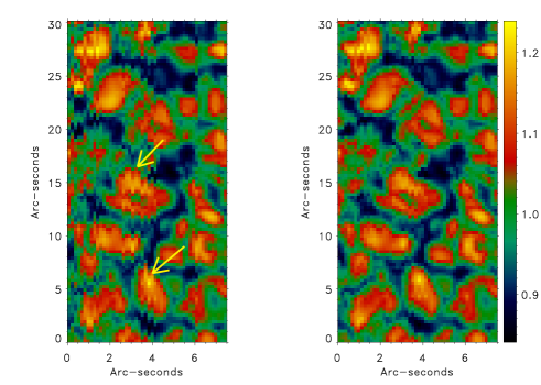
Figure 1: Detail of the continuum intensity in the observed field of view showing some glitches due to the sudden displacement of the frame along the slit direction (the arrows point to some of the most obvious examples). Left panel: Original image. Right panel: Corrected as explained in the text.

3 Analysis

For practical reasons, a smaller subfield of view of 200$\times$200 pixels has been selected for further analysis. This size is large enough to include abundant statistics on granulation and quiet Sun fields (including both network and internetwork) and at the same time small enough to allow a full inversion of each spatial point individually in a reasonable time span using a supercomputer. Figure 2 shows continuum intensity and a synthetic magnetogram (constructed simply as the absolute value of the circular polarization signal integrated over a 100 mÅ  range in the blue lobe of both lines) of the original full field of view and the subfield selected for inversion.

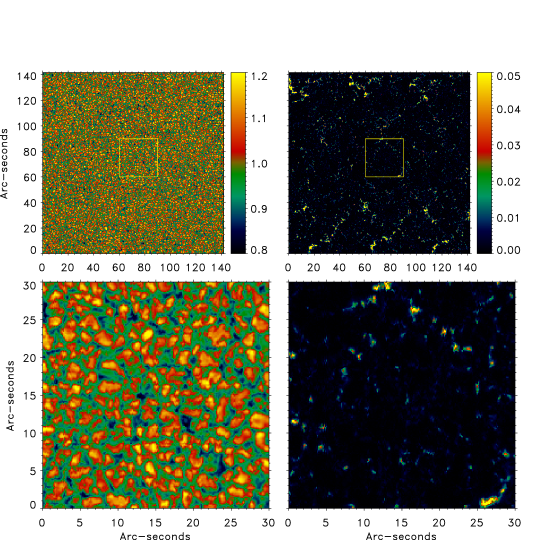
Figure 2: Full field of view (upper panels) and subfield selected for inversions (lower panels). Left: Continuum image. Right: Synthetic magnetogram, saturated at 5% of the average continuum intensity. The selected subfield avoids some flatfield artifacts that are visible as horizontal segments in the upper left panel.

The inversions were carried out with the code NICOLE (Socas-Navarro et al. 2010), which is an improved implementation of the original NLTE inversion code of Socas-Navarro et al. (2000). It makes use of response functions similarly to the popular LTE code SIR of Ruiz Cobo & del Toro Iniesta (1992), but has some features that are important for our purposes here. NICOLE is supported by a very wide variety of platforms and has built-in MPI parallelization, which makes the use of supercomputers rather simple and straightforward. Moreover, it has NLTE capabilities, including an option that is used for part of this work (see Sect. 3.1) in which it is possible to supply a (fixed) set of departure coefficients for the upper and lower levels of the spectral lines.

The calculations presented in this paper have been performed using the LaPalma supercomputer of the Instituto de Astrofísica de Canarias which harbors 512 64-bit processors, running at a speed of 2.2 GHz. A typical run, including the various passes described below, requires about 6 hours on 50 CPUs.

The observed spectral region contains two prominent Fe i lines (at 6301.5 and 6302.5 Å) whose profile shapes are fitted by the inversion code to find the optimal depth stratification of the atmospheric variables. These lines are well described with a LTE treatment (the effects of NLTE corrections will be analyzed in Sect. 3.1 below). The atomic parameters are taken from the VAL-D database (Piskunov et al. 1995), except for the transition probabilities. For the 6301.5 Å  line we use the laboratory measurements of Bard et al. (1991).

Unfortunately, no similar measurements exist for the 6302.5 Å  line and we derived it empirically in the following manner. We first inverted the 6301.5 Å  line in the FTS atlas mentioned above. With the model thus obtained we synthesized the 6302.5 Å  line adjusting the $\log(gf)$ parameter until a satisfactory fit to the observations was attained. Collisional broadening is treated with the formalism of Anstee & O’Mara (1995) with the parameters $\alpha$ and $\sigma$ obtained using the code of Barklem et al. (1998). The atomic parameters used are given in Table 1 ($r_{0}$ denotes de Böhr radius).

Table 1: Spectral line data

$$\begin{array}[]{ccccccc}\hline\cr\vskip 3.0pt plus 1.0pt minus 1.0pt\cr\lambda\ (\mbox{\AA})&Excitation&log(gf)&Term&Term&\sigma&\alpha\\ &pot.\ (eV)&&(lower)&(upper)&(r_{0}^{2})&\\ \vskip 3.0pt plus 1.0pt minus 1.0pt\cr\hline\cr\vskip 3.0pt plus 1.0pt minus 1.0pt\cr 6301.5&3.654&-0.718&{}^{5}P_{2}&{}^{5}D_{2}&834.4&0.243\\ 6302.5&3.686&-1.160&{}^{5}P_{1}&{}^{5}D_{0}&850.2&0.239\\ \vskip 3.0pt plus 1.0pt minus 1.0pt\cr\hline\cr\end{array}$$

For each pixel in the 200$\times$200 subfield, the inversion procedure takes a starting guess model atmosphere and iteratively modifies it by adding a correction (which, in general, is depth-dependent) to it, seeking the best fit to the observations with the synthetic profiles computed from that modified model. The correction that is applied to the guess model at each iteration may be constant with height (depth-independent), linear with $\log(\tau_{5000})$ (the logarithm of the continuum optical depth at 5000 Å) or it can be constructed as a concatenation of linear segments spanning the whole depth range. In this last case, the number of segments to use may be set arbitrarily by the user. In this manner, depending on the amount of information available, we can decide how much detail of the depth stratification we wish to retrieve. One needs to reach a compromise to adjust the amount of freedom in the model to the information available in the data. Too much freedom results in degeneracies and leads to uniqueness issues and other complications. On the other hand, being too restrictive results in poor fits and not extracting all of the available information. Usually, some experimentation with a few test cases is very useful to determine a nearly optimal set of parameters.

The choice of freedom in each physical parameter of the model (temperature, magnetic field, velocities, etc) is made in practice by selecting the number of inversion nodes (Ruiz Cobo & del Toro Iniesta 1992), which are actually the free parameters in the code. Using one node we have a depth-independent correction for the entire atmosphere. With two nodes we produce a correction that scales linearly with $\log(\tau_{5000})$. Similarly, with three or more nodes we produce more complicated variations. Following the recommendation of Ruiz Cobo & del Toro Iniesta (1992), we proceed in two successive cycles to improve convergence. We start in the first cycle with a relatively small number of nodes to obtain a first approximation to the solution, fitting the overall shape of the profiles. We then increase the number of nodes to obtain a better solution allowing more freedom to fit more subtle properties, such as line asymmetries.

In addition to these cycles, NICOLE implements a multiple-initialization scheme in which the inversion (both cyles) is repeated a number of times randomizing the initial guess. The process is stopped when a good fit is achieved or when a preset maximum number of inversions have been done. The criterion to decide what we consider a good fit and the maximum number of inversions are both defined by the user. This is helpful when, as in this case, one is batch processing a large number of profiles to minimize the risk of the algorithm settling in a secondary minimum. The price to pay for the ensuing improvement in stability is, of course, more CPU time. In the calculations presented here, the stopping criteria are: a)a fit better than 1% of the profile on average or b)up to five inversion attempts.

As a starting guess we take the HSRA model. Two different approaches are taken depending on whether the profile to invert exhibits significant polarization or not. In the first case, which accounts for 34% of the profiles, we consider two atmospheres coexisting side-by-side in the pixel, one magnetic and the other non-magnetic. To determine the non-magnetic component, we start with a preliminary inversion of Stokes $I$ only (weights for $Q$, $U$ and $V$ are set to zero) without any magnetic field. In this inversion we allow for some micro-turbulent line broadening to improve the fit since it is unlikely that the external atmosphere will be entirely field-free. However, we do not invert for a magnetic field here since our main focus is the field in the second component which is the one that gives rise to the Stokes $Q$, $U$ and $V$ profiles. The resulting model and Stokes $I$ profile from this preliminary inversion are then taken as the (fixed) external non-magnetic atmosphere in a subsequent inversion in which the filling factor is a free parameter. In the case that the pixel considered does not exhibit Stokes signal we proceed with a simple one-component inversion. The number of nodes employed in both cases is shown in Table 2. As mentioned above, only the first (preliminary) inversion has microturbulence so that the code is able to handle the extra broadening due to the magnetic field. In the second and third inversions, where the magnetic field is taken into account, microturbulence is set to zero.

Table 2: Inversion nodes

$$\begin{array}[]{lccccccccc}\hline\cr\vskip 3.0pt plus 1.0pt minus 1.0pt\cr&\vline&&Magnetic\,pixel&&&&\vline&Non-magnetic\,pixel&\\ Physical&\vline&Inversion1&&\vline&Inversion2&&\vline&\\ Parameter&\vline&Cycle1&Cycle2&\vline&Cycle1&Cycle2&\vline&Cycle1&Cycle2\\ \vskip 3.0pt plus 1.0pt minus 1.0pt\cr\hline\cr\vskip 3.0pt plus 1.0pt minus 1.0pt\cr Temperature&&3&5&&2&3&&3&5\\ L.o.s.\,velocity&&1&3&&1&2&&2&3\\ Microturbulence&&1&1&&0&0&&0&0\\ B_{long}&&0&0&&1&2&&0&0\\ B_{x}&&0&0&&1&2&&0&0\\ B_{y}&&0&0&&1&2&&0&0\\ Filling\,factor&&0&0&&1&1&&0&0\\ \vskip 3.0pt plus 1.0pt minus 1.0pt\cr\hline\cr\end{array}$$

In the table, $B_{long}$ refers to the longitudinal (i.e., along the line-of-sight) component of the magnetic field, whereas $B_{x}$ and $B_{y}$ are the transverse components, projected on the plane of the sky. The $x$-direction is the field azimuth reference, defined by the plane of vibration of light with $Q$$>$0 and $U$=0 in the calibration pipeline. The synthetic Stokes spectra computed at each step of the iteration are convolved with the instrumental profile of the Hinode SP (Lites, private communication) to make sure that synthetic and observed profiles are comparable.

A final pass is performed restarting the inversion with a smoothed version of the result to fix a small percentage of pixels that did not converge properly. The smoothing is done with a 3$\times$3 median box, but excluding the central point (i.e., the pixel to be re-inverted).

A sample of the resulting cubes can be seen in Fig. 3 which shows horizontal (in $\tau_{5000}$) cuts of the temperature and line-of-sight velocity at three representative heights in the photosphere. For the two-component inversions (pixels with magnetic signal), an average of the internal and external atmospheres weighted with their respective filling factors is shown.

The figure shows the characteristic convective motions at the base of the photosphere (top panels), with hot granules upflowing and cool lanes downflowing. The flow structure does not change too much until we reach the upper photosphere (bottom panel) in which the granulation pattern starts to dissolve leaving structures that vaguely appear to be vertically oriented. Since there is no preferred direction in the field of view, such structures are likely the result of observing a very dynamic upper atmosphere through a vertical slit. The temperature stratification starts with the granulation at the bottom but at $\log(\tau_{5000})$$=-1$ is dominated by hot patches in the magnetic areas embedded in a more uniform non-magnetic background. Finally, at the $\log(\tau_{5000})$$=-2$ height we start to see reversed granulation, where the photospheric granules are now cooler and the lanes are hotter.

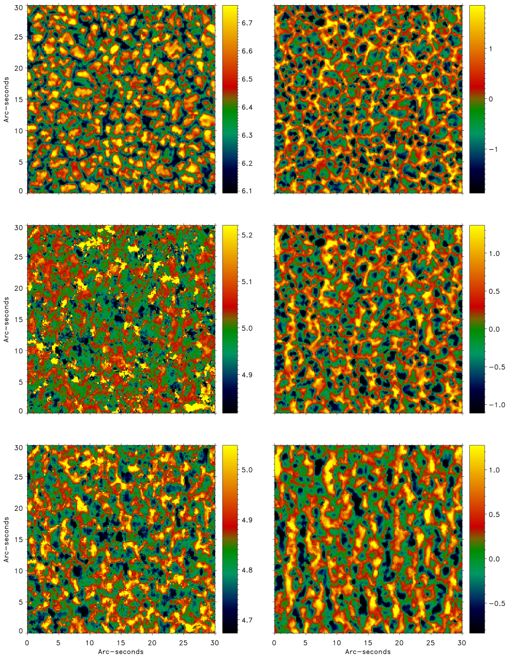
Figure 3: Horizontal cuts of the temperature (left) and line-of-sight velocity (right) at $\log(\tau_{5000})=0$ (top), $-1$ (middle) and $-2$ (bottom). Units are kK for temperature and km s^-1 for velocity. The astrophysical convention, where positive velocities indicate redshift (downflows), is adopted throughout this paper.

3.1 NLTE corrections

The Fe i lines used in this work are affected by (generally very small) NLTE effects (Shchukina & Trujillo Bueno 2001). Both the upper and lower levels of the transitions are slightly underpopulated with respect to their LTE values. This has virtually no effect on the source function, which goes with the ratio of the level populations, but produces a small overall decrease in the line opacity.

We introduce a correction for NLTE effects in the inversion scheme by using some departure coefficients computed by Shchukina & Trujillo Bueno (2001) in the 3D hydrodynamic model of Asplund et al. (2000, see also ). We take the run with $\log(\tau_{5000})$ of the departure coefficients for both levels of the 6301.5 and 6302.5 Å transitions computed by Shchukina & Trujillo Bueno (2001) in a typical granule and a typical lane in the 3D simulation. These values are then assigned to a particular granule and a lane pixel in the Hinode observations. For all other pixels we carry out a linear interpolation based on the continuum intensity. The departure coefficients obtained are kept fixed during the inversion, even though the atmospheric parameters change. While this method is not exact, it is a good approximation to correct for an effect that is already small anyway. A full NLTE solution for the Fe atom would be a tremendous undertaking and a full 3D inversion such as the one presented here would not be possible in practice due to the processing power required. With our approximation, the departure coefficients may be inconsistent with the starting guess atmosphere but as the inversion proceeds and approaches the solution, they become gradually more realistic.

4 Results

With the NLTE correction, the cores of the lines are fitted better and therefore the results for the upper layers are less noisy (see Fig. 4; compare bottom-left panel to that in Fig. 3). Figure 4 shows also the magnetic flux density in the region, revealing many internetwork field structures. The transverse flux density is more noisy because the Stokes $Q$ and $U$ signals are weaker than Stokes $V$ and correspondingly more difficult to detect. Nevertheless, we can see that a large fraction of the area harbors fields with a measureable horizontal component, in agreement with recent results such as those of Lites et al. (2008).

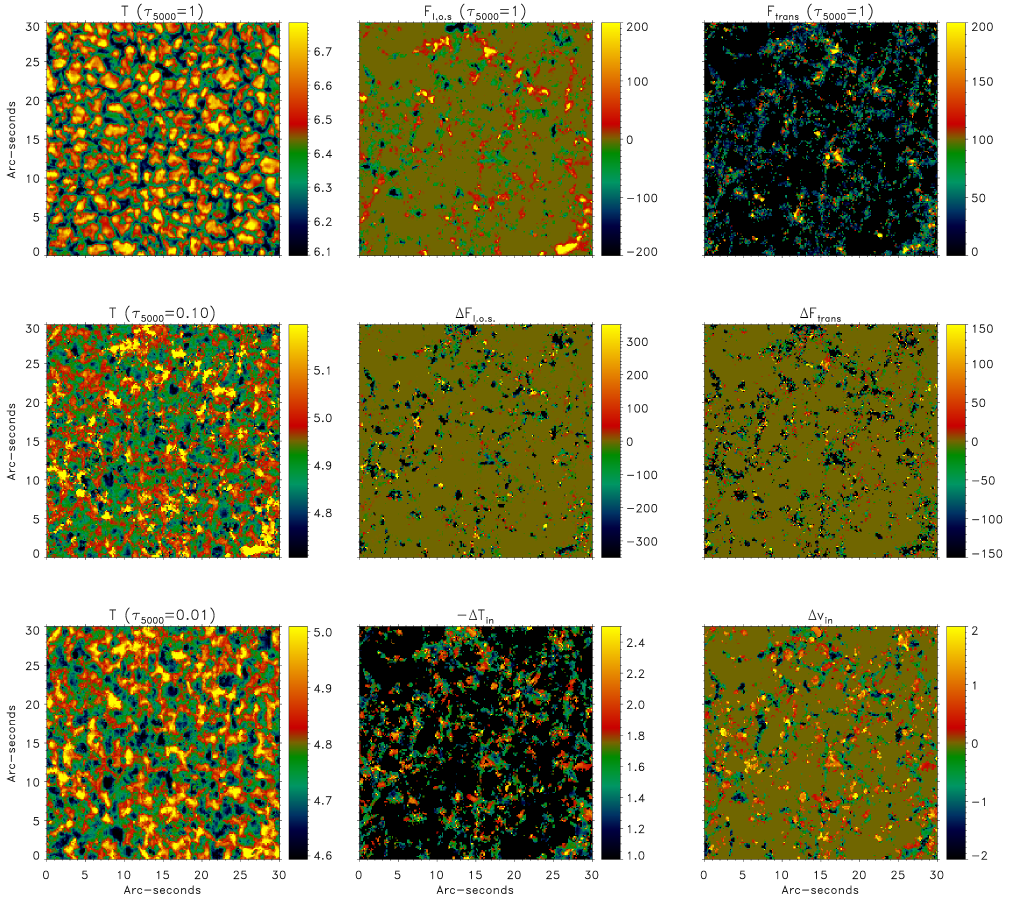
Figure 4: Horizontal (in the $\tau_{5000}$ depth scale) cuts of several interesting physical parameters in the multi-cube resulting from the inversion, including NLTE correction. The left column shows the temperature in kK at three different heights. The top row also shows the line-of-sight magnetic flux density (middle panel) in G and the transverse (on the plane of the sky) magnetic flux density (right panel) at the base of the photosphere. The middle row shows the variation of the flux density from $\log(\tau_{5000})$$=0$ to $\log(\tau_{5000})$$=-1$ (middle panel: line-of-sight component; right panel: transverse component). The bottom row shows the variation of the temperature in kK (middle panel) and the line-of-sight velocity in km s^-1 (right panel) from $\log(\tau_{5000})$$=0$ to $\log(\tau_{5000})$$=-1$ inside the magnetic atmosphere.

The magnetic field height gradient is mostly negative as one would expect. However, some concentratios show an increase of the field strength with height. Temperatures inside the magnetic atmospheres always decrease with height but there is a wide range of variation of $\sim$1 kK among various pixels. The mass flows may be upward or downward directed. However, the stronger flux elements are associated with downflows. If we consider pixels with a longitudinal magnetic flux stronger than 100 G, 84% harbor downflows and only 16% are upflowing. The external (non-magnetic) atmosphere is also undergoing downflows in those pixels.

Generally speaking, the fits to the individual profiles are good. Figure 5 shows the average intensity profile in the observed region and the average synthetic profile from the model. Notice that this is not actually a fit but an average of the 200$\times$200 individual fits.

We can also test the model against atlas observations. If we synthesize the profiles in the absence of macroturbulence and instrumental profile (i.e., with very high spectral resolution), we should obtain a profile very similar to that of an intensity atlas. In Fig. 6 we can see the comparison with the FTS atlas (Neckel & Labs 1984). Overall, the model reproduces the atlas observations with very high fidelity, including the line broadening. The absence of microturbulence does not represent any problem for obtaining realistic line shapes. This is not entirely surprising, since the observations have sufficient spatial resolution to resolve the granular components (granulation is the main contributor to the line broadening traditionally characterized by microturbulence in 1D models). It is, however, a noteworthy feature since the success in reproducing line widths without requiring any microturbulence has been remarked as a strong argument supporting theoretical 3D models derived in recent years.

Figure 5: Average intensity spectrum from the Hinode SP observed dataset (solid) and from the 3D model (dashed). Spectra are normalized to the continuum intensity ($I_{c}$).

Figure 6: FTS atlas intensity spectrum (solid) and average profile synthesized from the 3D model (dashed) without instrumental profile (i.e., with very high spectral resolution). The lines at 6302.00 and 6302.76 Å are telluric lines (absent in the Hinode data). Spectra are normalized to the continuum intensity ($I_{c}$).

When we compare the average temperature stratification of our model to others previously existing in the literature, we find that it is similar, although slightly cooler in the middle photosphere (some 100-200 K at $\log(\tau_{5000})$$=-1$) and warmer at the top ($\sim$150 K at $\log(\tau_{5000})$$=-3$). Figure 7 compares the horizontally averaged temperature to that of the Harvard-Smithsonian Reference Atmosphere (HSRA, Gingerich et al. 1971) and to the average temperature of Asplund et al. (2004). The HSRA is a semiempirical 1D model and one expects some differences with the one presented here because in principle the 1D model that fits a given spectral dataset is not necessarily the same as the average stratification of a 3D model that fits the same dataset. In other words, the HSRA already incorporates an empirical correction for 3D effects. The model of Asplund et al. (2004) is a 3D model but obtained from theoretical simulations. Compared to HSRA, it also produces an elbow around $\log(\tau_{5000})$$=-1$ but not as pronounced as our model. In the upper layers, on the other hand, both HSRA and the Asplund et al models are very similar in spite of the 1D vs 3D difference in approach and both are cooler than the present model.

Figure 7: Comparison of the average temperature stratification in our 3D model (solid line) to HSRA (dashed) and the average stratification of the Asplund et al. (2004) 3D model (dash-dotted).

The importance of 3D effects has been emphasized in recent work (e.g., Asplund et al. 2004) in the context of chemical abundance determinations. To assess the importance of 3D effects in our model we have compared the average emerging spectrum from what would be obtained if one first averages the atmospheric stratification and then compute the spectrum of such 1D average model. The results, displayed in Figure 8, are in this case rather small (but noticeable), with the main departure been at the core of the lines (i.e., affecting the upper atmospheric layers). The lines computed in 1D are also slightly narrower, which goes in the direction of compensating the change in equivalent width. In fact, the difference in equivalent width between the 1D and 3D profiles is at the 1.5% level.

Figure 8: Comparison of the average spectrum from the 3D model (solid) to the spectrum produced by the average model (dashed).

5 Uncertainties

It is important to estimate the errors and uncertainties in the derived model. Systematic errors may come from the normalization of the Hinode data since the observations are not photometrically calibrated. Instead, relative intensities to the disk-center average continuum have been employed, with the subsequent assumption that such disk-center average intensity is well reproduced by the HSRA model. The visible continuum is very sensitive to temperature variations, which has the advantage that it is relatively easy to determine the photospheric temperature. On the downside, a small error in the intensity calibration might have relatively large effects on the temperature determination. For instance, a 1% error in the continuum calibration results in a $\Delta$T of between 150 and 200 K (it is slightly different for granules and lanes). This example is particulary pessimistic, as we do not expect such a large error in the average intensity determination. Furthermore, the average temperature of our model at $\tau_{5000}=1$ (6441 K) is consistent with values from several other models existing in the literature, such as HSRA (6390 K) or those of Asplund et al. (2004, 6412 K), Holweger & Mueller (1974, 6530 K), Vernazza et al. (1981, 6424 K) and Fontenla et al. (1993, 6520 K).

5.1 Sensitivity range

Semi-empirical models derived from inversion of spectroscopic data, such as this one, are reliable only in the atmospheric region where the spectral lines exhibit some sensitivity to the physical parameters. A suitable way to explore this range is by using the so-called response functions (e.g., Ruiz Cobo & del Toro Iniesta 1994). Mathematically speaking, the response function of a given Stokes parameter at a given wavelength $I(\lambda)$ to perturbations in a given physical parameter at a certain height in the atmosphere $T(\tau)$ is expressed as:

$$R(\lambda,\tau)={dI(\lambda)\over dT(\tau)}\,.$$ (1)

Here we use the same nomenclature to refer to the discrete form (replacing the derivative with a ratio of finite increments) of Eq (1) which, albeit not entirely equivalent from the mathematical point of view, is very convenient in practical terms for our study. The most straightforward way to compute a response function is by brute force from its definition. We start with a reference atmosphere from which the emerging spectrum is known and then perturb this atmosphere, one point at a time, recompute the spectrum and calculate the ratio $\Delta I(\lambda)/\Delta T(\tau)$ (assuming that the perturbed variable is temperature at depth $\tau$). Response functions to temperature in a granule and an intergranular lane are displayed in Fig. 9.

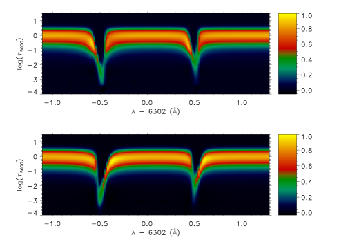
Figure 9: Normalized response functions $R(\lambda,\tau)$ to temperature in a granule (upper panel) and a lane (lower panel).

From the response functions we can already see that the sensitivity range of these two lines spans from roughly $\log(\tau_{5000})$$=0$ to $-3$, approximately. Let us go a step further and use this information to estimate the actual errors in the inversions. To this effect it is important to consider not only how sensitive the lines are but also how good a fit we have obtained. If we had only one wavelength, it is straightforward to see that the error in the determination of a given parameter (e.g., $T$ to fix ideas) may be approximated by $\Delta T=\Delta I/R$, where $\Delta I$ is the difference between the observed and the synthetic observable and $R$ is the response function.

Consider now a case with many wavelengths and assume for simplicity that the inversion result may be regarded as a weighted average of individual measurements of $T(\tau)$, one at each wavelength, all weighted by their individual response $R(\lambda,\tau)$. We can then use the expression for the variance of a weighted mean to obtain in our case:

$${1\over\Delta T(\tau)^{2}}=\sum_{\lambda}{R(\lambda,\tau)\over\Delta I(\lambda)}$$ (2)

Figure 10 shows the uncertainties in the temperature determination obtained using this expression in three different pixels of the field of view, which have been selected according to their continuum brightness to include a granule (bright point), an intergranular lane (dark point) and an average location. The residual discrepancy between the average observed and synthetic spectra is introduced in the equation as the $\Delta I(\lambda)$ function. The figure shows that extremely small errors ($\sim$10 K or smaller) are obtained for a fairly wide range of heights, between $\log(\tau_{5000})$$=0.5$ and -1.7, approximately. Up until $\log(\tau_{5000})$$=-2.5$ we can still have relatively small errors ($\sim$150 K) but above that height, measurements should be regarded as highly uncertain. Notice, however, that the dependence of the errors with the model atmosphere chosen is significant for the upper layers. The granule model is the one that has the error increasing more rapidly with height between $\log(\tau_{5000})$$=-2$ and $-3$. In the lane model the error increases more slowly. Finally, in the average atmosphere one can reach $\log(\tau_{5000})$$=-3.4$ with very small errors of $\sim$50 K.

Figure 10: Estimated uncertainty in the temperature stratification for three different model atmospheres. Solid line: Brightest continuum location in the field of view (a granule). Dashed line: Darkest continuum location in the field of view (a lane). Dotted line: A location having a brightness equal to the average of the whole region. Coordinates on the lower panel maps of Fig. 2 are (14.5,8.2) for the granule, (12.0,25.5) for the lane and (22.6,8.5) for the average brightness point.

5.2 Abundances

For the calculations in this work we have employed the solar chemical composition published by Grevesse & Sauval (1998). Since the spectral lines analyzed are from Fe transitions, this is the abundance value that will have a stronger impact on our results. The 7.50 value in Grevesse & Sauval (1998) seems to be very well established and, when NLTE effects are considered (Shchukina & Trujillo Bueno 2001), in good agreement with the meteoritic value. The rest of the elements are relevant only for the calculation of the background opacities.

To assess the impact of possible uncertainties in the abundances employed, the synthetic profile produced from the average model was inverted with different sets of abundances. A first test had the Fe abundance fixed and a constant scaling was applied to all other elements. The scaling factor ranged from 0.75 to 1.25. For the second test the Fe abundance was varied between 7.40 and 7.60, while the rest of the chemical composition was kept constant.

As expected, the only significant difference was found in the test where the Fe abundance was modified. Figure 11 shows the inversion with the reference value of 7.50 compared to the models obtained with the interval extremes (7.40 and 7.60, respectively). The changes are very small, mostly because the emerging intensity is extremely sensitive to temperature in this range. This means that a very small variation in the model temperature is able to compensate for significant variations in the line parameters. The upside of this conclusion is that semiempirical models such as the one presented here are rather robust and not very sensitive to uncertainties in line data, abundances, etc. Unfortunately, the downside is that abundance determinations are extremely sensitive to the model employed.

Figure 11: Models obtained when inverting the synthetic average spectrum with different values of the Fe abundance. The solid line is for the reference value of 7.50. The dashed lines are for 7.40 (lower curve) and 7.60 (upper curve).

6 Conclusions

The model presented here is novel in that it is three-dimensional in nature and has been obtained from real observations. It may hopefully serve as another platform for studies of chemical composition (in which more 3D models are urgently needed), to produce synthetic spectra (with or without polarization), analyze properties of the quiet Sun and their height variation or to learn about the physics of (magneto-)convection from direct comparison with numerical simulations.

This work may be improved upon by using new observations with even higher spatial resolution or more spectral features. Existing inversion codes such as NICOLE have the capability of incorporating lines from different elements and even to combine LTE and NLTE lines. It should be possible, in principle, to combine photospheric and chromospheric lines with the aim of producing a 3D model like this but spanning a much greater range of heights, all the way up to the middle chromosphere. The main limitation, however, is that we currently lack adequate instrumentation to produce such high-resolution multi-wavelength observations. Future planned ground-based telescopes such as the ATST (Keller et al. 2002) or the EST (Collados et al. 2010) or space-born observatories such as the plan B option of Solar-C (Hinode’s successor, still in early planning stages) would provide an enormous leap in our ability to acquire the necessary data.