Using Stellar Densities to Evaluate Transiting Exoplanetary Candidates

Abstract

One of the persistent complications in searches for transiting exoplanets is the low percentage of the detected candidates that ultimately prove to be planets, which significantly increases the load on the telescopes used for the follow-up observations to confirm or reject candidates. Several attempts have been made at creating techniques that can pare down candidate lists without the need of additional observations. Some of these techniques involve a detailed analysis of light curve characteristics; others estimate the stellar density or some proxy thereof. In this paper, we extend upon this second approach, exploring the use of independently-calculated stellar densities to identify the most promising transiting exoplanet candidates. We use a set of CoRoT candidates and the set of known transiting exoplanets to examine the potential of this approach. In particular, we note the possibilities inherent in the high-precision photometry from space missions, which can detect stellar asteroseismic pulsations from which accurate stellar densities can be extracted without additional observations.

1 Introduction

One of the principle goals of exoplanet searches using transits is the discovery of temperate terrestrial exoplanets. Their detection presents a tremendous challenge – particularly for the radial velocity observations that are typically used to confirm a transiting exoplanet candidate. Even the confirmation of transiting Hot Jupiters can confound observers, consuming and ultimately wasting telescope resources. Transit surverys typically identify 10-20 candidates for each planet (STARE, WASP (Pollacco et al., 2006), OGLE (Udalski et al., 2002a, b, c, 2003), HAT (Bakos et al., 2004)), although, in the case of CoRoT, the ratio of top priority candidates from that mission is closer to one-third or even one-half (Cabrera et al., 2009). This demonstrates the success of a decade-long effort to develop techniques to elminate transit candidates with further observations. Out-of-eclipse variations (Sirko & Pacyński, 2003), V-shaped vs. U-shaped transits (Pont et al., 2005), stellar density diagnostics (Seager & Mallén-Ornelas, 2003), and the Tingley-Sackett diagnostic (Tingley & Sackett, 2005), to name a few, have all contributed. Combined, these technique have enabled CoRoT’s relatively high success rate compared to, for example, the first OGLE run, which found 2 planets among 59 equally-prioritized candidates (Udalski et al., 2002a, b). Even so, many candidates defy easy characterization. CoRoT-7b (Léger et al., 2009), to use the lightest known transiting exoplanet as an example, required more than 100 observations with HARPS (Queloz et al., 2009), totalling over 70 hours of observing time. While the host star is fairly active in this case, thus complicating attempts to detect the radial velocity signal of the planet, the signal of CoRoT-7b was more than an order of magnitude larger than what one would expect for an Earth twin (3.3 m/s vs. 0.1 m/s). With the anticipated influx of candidates consistent with terrestrial exoplanets from both CoRoT and Kepler (and potentially future missions, such as PLATO), as well as from ground-based searches for transits across low-mass stars, any technique that could eliminate even a few terrestrial-class candidates would potentially save an enormous amount of valuable telescope resources.

One avenue of candidate screening that has not been fully explored is the density diagnostic first presented by Seager & Mallén-Ornelas (2003). Here, the authors demonstrated that it was possible to extract stellar densities by fitting the transit light curve with a simple trapezoid, which we will refer to in this paper as $\rho_{\rm SMO}$. At the time that paper was written, the required photometric measurements (5 mmag precision with 5 minute sampling covering two transits) was not at all typical for transit candidates – in fact, it was quite unusual. This paper was the first in what has turned into a long discussion on what exactly could be done with detailed analyses of transits. Tingley & Sackett (2005) proposed a technique to identify the best transit candidates in a sample using only transit periods, durations, and depths and included a discussion of the impact of unknown eccentricity on their technique. Barnes (2007) and Burke (2008) later expanded upon this secondary analysis to conclude that transits are more likely to occur in the elliptical orbits and this results in higher yields from transit surverys, respectively. Sozzetti et al. (2007) revisited one part of the Seager & Mallén-Ornelas (2003) derivation, stating that it was possible to obtain stellar densities from transit fits and that these could be used to aid in the derivation of stellar parameters from evolutionary tracks. Ford, Quinn & Veras (2008) showed that it was possible to estimate unknown eccentricites through an analysis of the transit shape; Kipping (2008) did something similar, deriving an entirely new equation that involved no potentially erroneous approximations. Yee & Gaudi (2008) worked to estimate period for transit candidates with but a single transit. Kipping (2010) compared the accuracy of different equations for transit duration, assessing the effect of incorrectly assuming circular orbits. Brown (2010) discussed the use of stellar densities from transits to restrict stellar radii, which are crucial in determining planetary radii.

In this paper, we combine and expand upon these ideas and propose a slightly different technique to identify good transit candidates: comparing densities calculated from transits to densities calculated by other, independent means, such as $J-K$ colors, spectra in combination with evolutionary tracks, and asteroseismology. It is our feeling that this will be of particular interest for shallow candidates discovered using ultra-high precision photometry from space-based mission such as CoRoT, Kepler and potential future missions such as PLATO for which the expected radial velocity signal would be weak and difficult to detect. To evaluate this technique, we use both the set of CoRoT candidates and the known transiting exoplanets to demonstrate that this diagnostic has the potential to be very effective in the pre-selection of the best candidates. To aid in this process, we derive a new equation for calculating stellar densities using other, more tangible transit parameters often available in papers that quote neither $a/R_{\star}$ nor the stellar density. This equation includes orbital parameters (eccentricity and angle of periastron), which make it possible to analyze the impact of an unknown orbital eccentricity on the measured stellar density. It is based on the equations in Sackett (1999) and Tingley & Sackett (2005) and may also be used as a consistency check of fitted transit parameters.

In $\S$ 2, we derive the equations that will be used for the analysis. In $\S$ 3, we discuss the independent density measures that compliment the stellar densities from transit parameters. In $\S$ 4, we apply these equations to those transiting exoplanets for which the necessary parameters have been published. In $\S$ 5, we examine the use of the $\rho_{\rm SMO}$ combined with the densities derived from $J-K$ colors on the CoRoT candidates. In $\S$ 6, we analyze the impact of eccentricity on this technique. Lastly, we discuss our conclusions in $\S$ 7.

2 Equations

Calculating the stellar densities from transit parameters is not difficult. The most straightforward way begins with the equation for the density of a spherical star:

$$\rho_{\star}=\frac{3M_{\star}}{4\pi R_{\star}^{3}}$$ (1)

where $\rho_{\star}$ is the density of the star and $M_{\star}$ is the mass of the star. Then, one can use Kepler’s 3rd law to substitute out $M_{\star}$, needing only the rather safe assumption that $M_{\star}\gg M_{p}$, obtaining an equation for the density of the star based on the transit parameter $a/R_{\star}$ ($\rho_{t1}$):

$$\rho_{t1}=\frac{3\pi}{GT^{2}}\left(\frac{a}{R_{\star}}\right)^{3}$$ (2)

where $G$ is the gravitational constant and $T$ is the orbital period of the planet (Seager & Mallén-Ornelas, 2003; Sozzetti et al., 2007). Despite the absense of parameters associated with orbital eccentricity, this equation does yield accurate stellar densities from transits of planets in elliptical orbits. Either the eccentricity and argument of the periastron are supplied from the analysis of the radial velocity observations and used during the transit fit or the radial velocity observations and the photometry are fit simultaneously.

It must be pointed out that $\rho_{t1}$ is distinctly different from $\rho_{\rm SMO}$, despite the fact that each are derived in the same article. $\rho_{t1}$ uses parameters extracted from a full transit fit with limb darkening to estimate the stellar density, while $\rho_{\rm SMO}$ uses a trapezoid fit to estimate the stellar density, neglecting limb darkening. Moreover, $\rho_{\rm SMO}$ assumes circular orbits, while $\rho_{t1}$ in principle takes into account eccentricity and the argument of the periastron.

It is possible to use $a/R_{\star}$ as a free parameter when fitting a transit, but many papers describing transit observations do not include it. Moreover, one cannot intuit whether the value makes sense from looking at a transit, which is clearly a problem in a few cases. Therefore, it is instructive and useful to derive equations for the stellar density and for $a/R_{\star}$ that depend on transit parameters that are tangible and more commonly published. Starting with Eq. 7 of Tingley & Sackett (2005) for the duration ($\tau_{14}$) of a planetary transit (itself derived from equations in Sackett (1999)):

$$\tau_{14}=2(R_{\star}+R_{p})\frac{\sqrt{1-e^{2}}}{1+e\sin\omega}\sqrt{1-\frac{a^{2}(1-e^{2})^{2}\cos^{2}i}{(R_{\star}+R_{p})^{2}(1+e\sin\omega)^{2}}}\left(\frac{T}{2\pi GM_{\star}}\right)^{\frac{1}{3}}$$ (3)

where $R_{p}$ is the radius of the planet, $e$ is the planet’s orbital eccentricity, $\omega$ is the argument of periastron, and $i$ is the orbital inclination. It assumes that the mass of the planet is negligible, the star-planet separation during transit is much greater than the stellar radius (which is not always the case), and the orbital velocity is constant during the transit. From inspection, it is evident that the right-hand side of above equation goes as $R_{*}M_{*}^{-1/3}$, which is proportional to $\rho_{*}^{-1/3}$. If we solve for $M_{*}^{1/3}/R_{*}$, cube everything and multiply by $4\pi/3$, we obtain another equation for the density ($\rho_{t2}$) of the parent star, based on more fundamental parameters than $a/R_{\star}$:

$$\rho_{t2}=\frac{3TQ^{3}}{\pi^{2}G\tau_{14}^{3}}\left(\frac{(1+k)^{2}-b^{2}}{1-e^{2}}\right)^{\frac{3}{2}}$$ (4)

where the ratio of the radii $k=R_{p}/R_{\star}$, the impact parameter $b=Qa\cos i/R_{\star}$ and

$$Q=\frac{1-e^{2}}{1+e\sin\omega},$$ (5)

which equals 1 for circular ($e=0$) orbits. One can also solve the same equation for $a/R_{\star}$, getting:

$$\frac{a}{R_{\star}}=\frac{TQ}{\pi\tau_{14}\sqrt{1-e^{2}}}\sqrt{(1+k)^{2}-b^{2}}.$$ (6)

Plugging this equation into Eq. 2 yields the same results as given in Eq. 4 . As this equation is invertible, transit durations can be calculated from $a/R_{\star}$ as well. This makes it possible to check the quality of a fit in cases where all of the pertinent parameters ($T$,$\tau_{14}$, $a/R_{\star}$, $b$, $k$, $e$, $\omega$) are given. Additionally and significantly, this equation makes it possible to evaluate the potential impact of an unknown orbital eccentricity on densities determined from transit parameters (referred to generically as transit densities or $\rho_{t}$ hereafter).

With these two equations in hand, we can assess if the assumption of $a\gg R_{\star}$ is an issue – indeed Kipping (2010) specifically calls into question the accuracy of this equation – but given the level of uncertainty in transit parameters, it ultimately make little discernable difference. HAT-P-7b has one of the smallest $a/R_{\star}$s, only 3.82 (Winn et al., 2009a). Even for this case, the impact on the density is very small: $\rho_{t1}=0.217$ and $\rho_{t2}=0.204$ – only 6%, which is approximately one-third the size of the measurement errors and not an atypical difference between $\rho_{t1}$ and $\rho_{t2}$ for the transiting exoplanets for which both values are available. However, planets may someday be discovered transiting very closely to evolved or very hot stars – for such cases, this assumption might very well prove problematic.

3 Independent Stellar Density Measures

In order to accomplish our stated goal of evaluating transit candidates by their stellar densities, it is necessary to have an independent measure of stellar density to compliment the transit density. In the following analyses, we pursue three different possibilities: 1) from published values of stellar radii and masses not based on transits, 2) from $J-K$ colors, and 3) from asteroseismology. As a group, these will hereafter be referred to as stellar densities.

3.1 Stellar Densities from Published Stellar Masses and Radii

It is a trivial matter to calculate stellar densities from the published stellar masses and radii (referred to hereafter as $\rho_{spec}$). These are generally derived from spectral analysis combined with modeled evolutionary tracks (see Sozzetti et al. (2007) for a detailed discussion). Spectral analysis yields a variety of information, such as temperature, metallacity, $\log g$ (where $g=GM_{*}/R_{*}^{2}$), which can then be used with either a true distance measure (generally from Hipparcos) or evolutionary tracks to obtain the stellar radii and densities, using $\rho_{*}/\rho_{\odot}=g_{*}/g_{\odot}R_{*}$. According to Sozzetti et al. (2007), it is possible to use $\log g$ to constrain the stellar parameters from the evolutionary tracks, but surface gravities from spectra generally are not very precise, leading to highly uncertain stellar radii. They then proposed using transit densities to improve the determination of stellar parameters. This would suggest that at least some groups have used the transit densities to help determine their stellar parameters; while it was not done before the TrES-2 paper (Sozzetti et al., 2007), it has in the intervening years become essentially universal. Therefore, we caution that for some published transiting exoplanets, this density ($\rho_{spec}$) may not be truly independent of the transit density.

3.2 Stellar Densities from $J-K$ colors

Allen’s Astrophysical Quantities (Cox, 2000) lists $J-K$ colors and stellar masses and radii as a function of spectral type for main sequence stars. While these values are very general, being independent of factors such as age and metallicity, they may offer a reasonable approximation of stellar density, at least for the purpose of identifying less-than-ideal candidates. The advantage of this measure is that $J-K$ colors are readily available for most stars from the 2MASS database (Skrutskie et al., 2006), which means that no additional observations or analysis are necessary – simply look up the $J-K$ color, then interpolate among the values from Allen’s Astrophysical Quantities to arrive at the density ($\rho_{JK}$) considering only main sequence stars. This is illustrated in Fig. 1, which plots the stellar density versus the $J-K$ color.

Apparently, this measure has several weaknesses. First, it assumes that all stars are main sequence stars. Obviously, this is not always the case; stars evolve, and once off the main sequence the resulting $J_{K}$ densities would be incorrect. Second, while $J-K$ is a very red color, stars residing in dust-rich environs can experience enough interstellar reddening to have a significant effect on their resulting density. For example, CoRoT-10b has color excess $E(J-K)=0.24$ (Bonomo et al., 2010), which leads to a difference in $\log(\rho_{\star}/\rho_{\odot})$ of about 0.5 dex – or a factor 1.6.

Figure 1: $J-K$ colors and spectral types vs. stellar density. This figure shows how the stellar density varies with $J-K$ color and spectral type for the main sequence. Diamonds show the actual values from Allen’s Astrophysical Quantities (Cox, 2000), while the line and asterisks show the interpolated values (a fourth-degree polynomial fit) used to calculate the $J-K$ stellar densities used in this paper.

Technically speaking, the 2MASS $J$ and $K$ colors are slightly different than the Bessel and Brett Bessel & Brett (1988) system used in Allen’s Astrophysical Quantities. Therefore, to be completely rigorous, a conversion from the one system to the other ought to be performed. However, such a conversion results in a very small change in stellar density – only a few hundreds of a solar density. Considering the magnitude of the generalizations involved in this density measure, this difference can be neglected.

3.3 Asteroseismic Densities

Another technique exists that can reliably obtain stellar densities, though we cannot exploit it yet in this work: asteroseismology. By measuring the frequencies of the acoustic modes and performing some model-fitting, it is possible to get a good measure of the stellar density from the average frequency spacing between these modes in the asymptotic region (Vandakurov, 1967; Tassoul, 1980). It is only in the last few years that these measurements have become possible, generally through the radial velocity fingerprint of these oscillations (e.g. Kjelsen, Bedding, & Christensen-Dalsgaard (2008)). Recently, however, circumstances have changed: the Kepler satellite mission has the capacity to obtain photometric time series with the necessary precision to reveal stellar oscillations, as would proposed missions in the future such as PLATO. This is potentially very interesting: the photometric precision necessary to discover transiting terrestrial exoplanets should also be sufficient to detect oscillations, thereby offering a sensitive density measure without additional observation.

4 Application to Known Transiting Exoplanets

We performed an extensive literature search to gather the transit parameters for as many transiting exoplanets as possible. Table 1 lists the planets and their periods, along with their corresponding $\rho_{t1}$ and $\rho_{t2}$ (calculated from the available transit parameters) and $\rho_{JK}$, when possible – some faint (or very crowded) candidates do not appear in the 2MASS database. Asteroseismic densities are much less common, however: only a single recent paper by Christensen-Dalsgaard et al. (2010) publishes asteroseismic densities ($\rho_{a}$), and then only for the three stars known to harbor exoplanets in the Kepler field before the mission began: HAT-P-7, HAT-P-11, and TrES-2 – the last two with preliminary stellar parameters only. These are also included in Table 1.

Fig. 2 shows the ratio of the transit densities and the stellar densities from masses and radii, with $\rho_{t1}$ on the top and $\rho_{t2}$ on the bottom. These figures demonstrate that, for nearly all of the candidates, the two values agree within the errors bars – even the eccentric ones. If anything, they agree far more than we would expect from the size of the error bars – evidence that the practice of using transit densities to constrain model fits of stellar parameters is widespread. Only four planets seem to have deviations greater than $1\sigma$ from a density ratio of one for either $\rho_{t1}/\rho_{spec}$ or $\rho_{t2}/\rho_{spec}$: HAT-P-7b, CoRoT-11b, CoRoT-7b and OGLE-TR-211b. The first case is resolved when the transit parameters are taken from the same reference as the stellar parameters (Pál et al., 2008), instead of a later paper (Winn et al., 2009a), which contains better photometry and consequently more precise transit parameters but does not repeat the spectral analysis of the parent star. This presents a clear case where the derived transit density influences the stellar parameters. The second offers no easy explanation and requires further study. The last two do not have sufficiently precise photometry for confident parameter estimation: CoRoT-7b has an extremely shallow transit and it has been further hypothesized that magnetic activity or transit timing variations may affect the shape of the transit (Léger et al., 2009) and OGLE-TR-211b has not been observed well enough – several different transits are spliced together to create the final light curve, introducing undefined uncertainties. This emphasizes the fact that good photometry without significant unknown systematics is essential for the use of this technique.

As can be seen in Fig. 3, the details of the distribution of the density ratios is interesting. The region is largely triangular, with a narrower distribution for deep transits and wider for shallower ones. This apparent dependency could arise from two causes: underestimations of $\rho_{t1}$ and $\rho_{t2}$ or overestimation of $\rho_{JK}$. It is unlikely that bad transit parameters are the source of this problem: while shallower transits would tend to have less precise transit parameters, the precision of the transit parameters for the CoRoT planets is more limited by uncertainties in the limb darkening parameters than photometric precision and they exhibit the same tendency. Therefore, we suspect that $\rho_{JK}$ is the source. Most of the planets – but of course not all – discovered are approximately Jupiter-sized. Therefore, some fraction of shallower transits correspond to larger (evolved) stars. The $\rho_{JK}$s derived are based on the assumption that the stars are still on the main sequence. If the $J-K$ colors accurately represent the densities of main sequence stars, some of the larger stars will be more evolved stars, rather than higher mass, explaining the presence of unexpectedly low density ratios, leading to the observed increase in the spread in density ratios as transit depth decreases. The numbers actually bear this out; the four exoplanets with the lowest density ratios (HAT-P-4b, HAT-P-13b, HD 149026b, and HD 17156b) have orbit stars with effective temperatures between 5650 and 6150 Kelvin, but $R\sim 1.5R_{\odot}$ and $\log g\sim 4.2$, when $\sim 4.5$ is more typical for main sequence stars with these temperatures – indeed, HD 149026b is classified as a subgiant.

Asteroseismic densities may be more accurate than $\rho_{JK}$, the few known examples exhibiting little scatter around the expected density ratio of unity. While the current sample is too small for conclusions, we note that additional observations are not necessary to obtain the asteroseismic density, only some analysis. Therefore, a comparison between asteroseismic densities and transit densities, when possible, should prove to be an extremely valuable diagnostic tool in evaluating transit candidates. This may be particularly useful for candidates for terrestrial exoplanets in multi-planet systems – some groups have hypothesized that terrestrial planets may favor low-eccentricity orbits to maintain stability, both with giant planets present (Pilat-Lohinger, 2009) and without (Mann, Gaidos, & Gaudi, 2010). This topic is still being debated, however, and does not address single planet systems al all.

Figure 2: The left-hand figure shows the density ratios for the known transiting exoplanets for which the necessary information is available. Density ratios are created using spectra ($\rho_{\star}$) and either $\rho_{t1}$ (top) or $\rho_{t2}$ (bottom). Notice how consistently these values are centered around 1, particularly for $\rho_{t1}$ – clear evidence of the widespread use these densities have in the final determination of stellar parameters. The right-hand figure reiterates this with a comparison of the density ratios calculated using $\rho_{t1}$ and $\rho_{t2}$ for the subset of transiting exoplanets for which all the necessary parameters are published. Note that the values for $\rho_{t1}$ and $\rho_{t2}$ are very similar in most cases, even for planets with high eccentricities, verifying that $\rho_{t2}$ is accurate. Those that appear to be outliers actually aren’t – the errors bars are large enough to include the anticipated result. Those that deviate from ratios of 1 but remain close to the overplotted line probably have problems obtaining the stellar parameters from the spectra (and models), while those that are displaced upwards and downwards typically have problems with the photometry.

Figure 3: $\rho_{transit}/\rho_{\star}$ vs. transit depth for known exoplanets. This figure shows the density ratios (in this case, $\rho_{t1}/\rho_{JK}$, when available, otherwise $\rho_{t2}/\rho_{JK}$) for all the known transiting exoplanets (squares) and for the three cases for which the asteroseismic density ($\rho_{t1}/\rho_{a}$ or $\rho_{t2}/\rho_{a}$ is known (diamonds)). The depth is approximated as the square of the planet-star radius ratio. The known exoplanets have density ratios distributed in a way that appears to be asymmetric relative to the ideal $\rho_{transit}/\rho_{\star}=1$ value, likely due to stellar evolution (shaded region). The limited sample of asteroseismic densities appears to be more reliable, agreeing well with the transit densities regardless of transit depth.

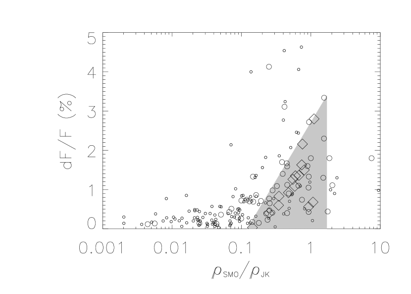
Figure 4: $\rho_{transit}/\rho_{\star}$ vs. transit depth plot for the CoRoT candidate list. Diamonds are the confirmed exoplanets, while large circles are the highest priority CoRoT candidates and small circles lower-priority CoRoT candidates. For these, $\rho_{\rm SMO}$ is the transit density estimated by the trapezoid method and $\rho_{JK}$ is the stellar density. The shaded region is the same as in Fig. 3. Notice how the CoRoT planets fall in the same shaded region. Also notice that the vast majority of candidates have very low density ratios, while very few have ratios higher than 1. This is because candidates in both giant stars and significantly blended stars will have low density ratios (Seager & Mallén-Ornelas, 2003), while only eccentricity or errors can increase density ratios. This demonstrates how effectively density ratios can be for screening transit candidates. It also shows that $\rho_{\rm SMO}$ is a reasonable proxy for $\rho_{t1}$ and $\rho_{t2}$.

Figure 5: Density Ratio vs. eccentricity and angle of periastron. This figure shows how the density ratio varies as a function of angle of periastron and eccentricity. The lines from outermost to innermost depict eccentricities going from 0.9 to 0 in steps of 0.1. Notice how the angle of periastron produces density ratios greater than 1 over a larger range of values than it does for ratios less than 1.

Figure 6: Density ratio vs. probability and eccentricity. This figure shows the probability of measuring a particular density ratio as a function of eccentricity. The lines from innermost to outermost depict eccentricities going from 0.9 to 0.1 in steps of 0.1. Notice how the probability that the density ratio is greater than 1 increases with eccentricity.

Figure 7: Density ratio probabilities vs. period. This figure shows the probability that a transiting planet with unknown $e$ and $\omega$ will produce a given density ratio for three different period regimes, using the observed distribution of exoplanet eccentricities. The dashed line is for planets with periods less than 5 days, while the dotted line is for planets with periods of 5 to 100 days and the solid line is for planets with periods longer than 100 days. Notice how the peak at a density ratio equal to one decreases as period increases, while the chance for extreme density ratios increases. Please note that the lines have been smoothed for clarity.

Figure 8: Density ratio probabilities vs. eccentricity. This figure shows the probability that a given eccentricity with an unknown periastron angle will have a transit density lower than the listed value. The eccentricity ranges from 0.1 to 0.9 in steps of 0.1. From this plot, it is clear that high eccentricities strongly favor transit densities greater than 1, while low-to-moderate eccentricities have a significant probability of producing comparatively low density ratios. Arbitrarily choosing a density ratio cut-off of $\geq 0.5$ would falsely de-prioritize $\sim$ 11% of transits with an eccentricity of 0.7, , $\sim$16% of transits with an eccentricity of 0.4 and no transits with an eccentricity less than about 0.22, while including relatively few astrophysical false positives. It should also be mentioned that low eccentricities $<0.3$ are more common, particularly for exoplanets with periods less than 5 days – which transit searches are most likely to find.

5 Application to CoRoT Candidates

The set of CoRoT candidates offers an excellent opportunity to test this technique. Many of these candidates are listed in papers describing the results of individual CoRoT runs – e.g. IRa02 (Carpano et al., 2009) and LRc01 (Cabrera et al., 2009) – but others are not yet published. Ideally, we would want to use transit densities calculated from detailed transit fits and compare them to densities from spectra, but this information is not currently available for more than a handfull of candidates. However, as part of the array of information used for ranking candidates, the CoRoT Science Team determines both $\rho_{\rm SMO}$ (derived from a trapezoid fitting that neglects limb darkening) and $\rho_{JK}$. Each of these techniques is somewhat less than ideal, but without spectral information for each candidate, it is impossible to use detailed transit fitting including limb darkening and stellar evolutionary tracks to get better densities. They are apparently sufficient, however, to test the potential of density for candidate evaluation. As can be seen in Fig. 4, these simple density measures work remarkably, perhaps even surprisingly, well. While not all of the planets line up along the line describing the density ratio $\rho_{\rm SMO}/\rho_{\star}=1$, most of the planets do however fall in or are very close to the same well-defined region as the planets shown in Fig. 3. We note that the follow-up process is incomplete and that some of the candidates in that region may in fact be unconfirmed planets.

It is also clear in this figure that the majority of candidates have very low density ratios. This can be primarily attributed to two causes beyond the limitations of $\rho_{\rm SMO}$: giant stars and blends, which are eclipsing binaries whose light is accompanied by a bright third star, causing deep eclipses to be diluted and thus appear like planetary transit. As already mentioned in Seager & Mallén-Ornelas (2003), both blends and giant stars will have unusually low values of $\rho_{\rm SMO}$ – the giants stars because their density is truly much lower than main sequence stars and the blends because the inclusion of the light of the third star leads the trapezoid fit to converge on a solution that is larger than the bright third star and with a higher impact parameter. This overestimation of the radius leads in turn to an underestimation of the stellar density of the third star of up to 50%.

The known planets in this figure support the hypothesis that the distribution of densities ratios is due more to the insufficiency of $\rho_{JK}$ than the transit densities. The precision of CoRoT data is extremely high, so the errors in the transit parameters are dominated by uncertainties in the limb darkening rather than limitations of the photometry. Indeed, despite the fact that $\rho_{\rm SMO}$ is built upon more risky assumptions than $\rho_{t1}$ and $\rho_{t2}$ and therefore presumably less reliable, the distribution of the $\rho_{\rm SMO}$ densities for the CoRoT planets are essentially indistinguiable from the distribution of the $\rho_{t1}$ and $\rho_{t2}$ densities for all exoplanets (including the CoRoT planets) – while the individual values are different, the distribution is not. The only exception is CoRoT-7b, for which the extracted transit parameters are likely distorted by magnetic activity or transit timing variations. This demonstrates that $\rho_{\rm SMO}$ is actually quite useful in and of itself (particularly for more central transits) given the errors inherent in the extracted transit parameters, which may or may not include impossible-to-define uncertainties in limb darkening coefficients.

6 Impact of Eccentricity on Densities from Transits

As the transit density is a function of the orbital eccentricity and angle of periastron, the danger in using this diagnostic blindly is the high probability of a significantly non-zero eccentricity – most planets have significant eccentricity, particularly among planets with periods greater than 5 days or so. To evaluate the value of this technique properly, it is necessary to evaluate the influence of non-zero eccentricities.

It is a relatively straightforward matter to use the equation for $\rho_{t2}$ (which directly includes eccentricity while the equation for $\rho_{t1}$ does not) to explore this dependency. By comparing the response of $\rho_{t2}$ as $e$ and $\omega$ are changed to $\rho_{t2}$ with $e=0$, we can observe the effect of unknown eccentricity on the $\rho_{t2}(e,\omega)/\rho_{t2}(e=0)$ density ratios. This is shown in Fig. 5. These can readily be converted into the probability of observing a particular density ratio as a function of $e$, if $\omega$ is unknown. This is shown in Fig. 6. Here, we see that, as eccentricity increases, the probability of observing a density ratio greater than 1 increases. This is the case because the probability that a transit occurs goes as the inverse of the star-planet separation, which therefore more likely that a transiting planet will transit when it is close to its parent star, rather than far away. The closer the planet is to its parent star, the higher its orbital velocity relative to its hypothetical $e=0$ velocity. Higher velocities lead to shorter transit durations and thus higher transit densities. The higher the eccentricity, the more pronounced this effect: 93.9% of all orbits with $e=0.9$ will produce a density ratio greater than 1. This can then be combined with the observed distribution of planet eccentricities as a function of period (Fig. 7), to give an idea of what fraction of planets with a given density ratio and period are planets. It is important to remember that this sample is comprised almost entirely of giant planets, however – the distribution of eccentricity as a function of period might be different for terrestrial planets.

One final consideration must be remarked upon: while density ratios larger than 1 are more common for planets of unknown eccentricities, very low density ratios will also occur, albeit rarely. These will exhibit very distinctive light curves that display very long, flat-bottomed transits. A density ration of 0.01 would result in an increase in the duration by a factor of $\sqrt[3]{1/0.1}=4.6$ over that expected for a circular orbit with the same period. Given that planets in circular orbits with periods of a year would have transit durations over 12 hours, such planets could have transit durations up to several days, but would stand out among false positives with similar density ratios. To the best of our knowledge, only eclipses of giant stars could produce similar events and these can be quickly identified with spectra due to their low surface gravity. For the interpretation of transit candidates, this means that cases with low $\rho_{t}/\rho_{JK}$ (or $\rho_{t}/\rho_{a}$, if available) should first be studied to see if the prospective parent star is a giant. If not, the probability that the candidate is a planet remains very low (see Fig. 8) and should thus be assigned a very low priority.

To apply this method, we recommend selecting a lower limit for the density ratio as a function of the period: only planets with periods $\gtrsim 100d$ are currently known to have a chance to have very extreme eccentricities; in fact, the maximim possible eccentricity dereases with period: $e\lesssim 0.35\log(T/1d)+0.24$ (based on figure 4 from Deeg et al. (2010)). Accordingly, no known ’hot’ planets ($T<5d$) have an eccentricity higher than 0.265. With this in mind, we can therefore conclude, per Fig. 8, that all candidates with density ratios lower than 0.45 can be strongly de-prioritized. Similar ’secure’ cut-offs could be established for candidates with longer periods, which could potentially possess larger eccentricities. Additionally, ’semi-secure’ cut-offs could be implemented, which would have small residual probabilities of falsely de-prioritizing very eccentric planets. However, should $\rho_{JK}$ be used to create the density ratio, it is perhaps better to be more circumspect given this density measure’s difficulties with evolved stars.

7 Conclusions

Ratios of densities derived from transit parameters over those from $J-K$ colors (or some other independent measure, such as asteroseismology) are a useful tool for the identification of transit exoplanets out of a much larger set of candidates. Even rudimentary density measures (trapezoidal and $J-K$ densities) appear to identify exoplanets effectively among the CoRoT candidates. More precise density measures from detailed transit fitting and stellar spectra will be even more effective; these, however, require additional spectral observations. Given data of sufficient quality, densities from asteroseismology might be even more effective, although at this time the sample of systems with transiting exoplanets and asteroseismic densities is too small to draw a definitive conclusion. Significant eccentricities will impact the measured density ratio in the absense of any knowledge of these orbital parameters; however, they will tend to increase the density ratios of discovered transiting exoplanets, while most false positives have density ratios lower than typical planets. It is important to remember that any tool can be misused; the one describe in this paper is no exception, but it does represent an improvement on other techniques currently used to prioritize transit candidates using transit parameters. Even a ’secure’ density cut-offs as described in the previous section may de-prioritize some true exoplanets due to any number of causes: extreme planet or star characteristics or otherwise inaccurately measured density ratios, for example. However, when used in conjunction with other techniques (ellipsoidal variations, presence of secondaries, etc.), density ratios can help identify the candidates which are most likely to be exoplanets and which are most likely to be false positives, increasing the efficiency of efforts to confirm or reject planet candidates.

Table 1.— Stellar densities (in ${\rm g\,cm}^{-3}$)
Planet	reference	$\rho_{t1}$	$\rho_{t2}$	$\rho_{JK}$	$\rho_{s}$	$\rho_{a}$
CoRoT-1b	Gillon et al. (2009a)	$0.87^{+0.40}_{-0.09}$		1.19	$1.21^{+0.42}_{-0.31}$
CoRoT-2b	Alonso et al. (2008)	$1.87^{+0.03}_{-0.03}$		1.57	$1.87^{+0.16}_{-0.16}$
CoRoT-3b	Deleuil et al. (2008)	$0.50^{+0.08}_{-0.07}$		1.21	$0.51^{+0.10}_{-0.09}$
CoRoT-4b	Aigrain et al. (2008)	$1.17^{+0.05}_{-0.01}$		1.25	$1.02^{+0.09}_{-0.03}$
CoRoT-5b	Rauer et al. (2009)	$0.87^{+0.08}_{-0.06}$		1.43	$0.85^{+0.09}_{-0.08}$
CoRoT-6b	Frilund et al. (2010)	$1.38^{+0.08}_{-0.12}$	$1.38^{+0.08}_{-0.07}$	1.43	$1.38^{+0.13}_{-0.12}$
CoRoT-7b	Léger et al. (2009)	$2.75^{+0.60}_{-0.57}$	$2.02^{+0.30}_{-0.27}$	1.61	$1.99^{+0.31}_{-0.26}$
CoRoT-8b	Bordé et al. (2010)	$2.67^{+0.19}_{-0.18}$	$2,23^{+0.15}_{-0.16}$	2.12	$2.72^{+0.26}_{-0.24}$
CoRoT-9b	Deeg et al. (2010)	$1.68^{+0.17}_{-0.16}$	$1.68^{+0.17}_{-0.16}$	1.43	$1.68^{+0.18}_{-0.17}$
CoRoT-10b	Bonomo et al. (2010)	$3.32^{+0.73}_{-0.64}$	$3.51^{+0.97}_{-0.86}$	2.54	$2.55^{+0.57}_{-0.45}$
CoRoT-11b	Gandolfi et al. (2010)	$0.69^{+0.02}_{-0.02}$	$0.67^{+0.03}_{-0.03}$	1.43	$1.13^{+0.18}_{-0.18}$
CoRoT-12b	Gillon et al. (2010)		$1.22^{+0.13}_{-0.14}$	1.43	$1.10^{+0.33}_{-0.25}$
CoRoT-13b	Cabrera et al. (2010)	$1.47^{+0.13}_{-0.13}$	$1.18^{+0.07}_{-0.07}$	1.26	$1.49^{+0.14}_{-0.13}$
CoRoT-14b	Tingley et al. (2010)	$0.90^{+0.17}_{-0.15}$	$0.85^{+0.12}_{-0.12}$	1.64	$0.09^{+0.22}_{-0.17}$
GJ 436b	Shporer et al. (2009a)		$6.81^{+0.78}_{-0.72}$	4.05	$7.00^{+1.04}_{-0.88}$
GJ 1214b	Charbonneau et al. (2009)		$23.9^{+2.1}_{-1.9}$	20.9	$23.6^{+4.6}_{-4.1}$
HAT-P-1b	Winn et al. (2007b)	$1.12^{+0.67}_{-0.73}$	$1.14^{+0.11}_{-0.10}$	1.15	$1.14^{+0.17}_{-0.15}$
HAT-P-2b	Pál et al. (2010)	$0.43^{+0.06}_{-0.05}$	$0.43^{+0.06}_{-0.06}$	0.80	$0.44^{+0.07}_{-0.06}$
HAT-P-3b	Torres et al. (2007)	$2.69^{+0.53}_{-0.53}$	$2.67^{+0.58}_{-0.53}$	1.60	$2.36^{+0.34}_{-0.37}$
HAT-P-4b	Kovács et al. (2007)	$0.434^{+0.002}_{-0.002}$	$0.446^{+0.039}_{-0.007}$	1.25	$0.44^{+0.07}_{-0.07}$
HAT-P-5b	Bakos et al. (2007)	$1.02^{+0.06}_{-0.07}$	$1.03^{+0.08}_{-0.08}$	1.34	$1.03^{+0.15}_{-0.13}$
HAT-P-6b	Noyes et al. (2008)	$0.57^{+0.04}_{-0.04}$	$0.58^{+0.05}_{-0.05}$	0.97	$0.59^{+0.08}_{-0.07}$
HAT-P-7b	Pál et al. (2008)	$0.29^{+0.06}_{-0.06}$	$0.32^{+0.08}_{-0.07}$	0.89	$0.33^{+0.07}_{-0.10}$	$0.2712\pm 0.0032$
	Winn et al. (2009a)	$0.20^{+0.07}_{-0.02}$	$0.22^{+0.07}_{-0.03}$	0.89	$0.33^{+0.07}_{-0.10}$
HAT-P-8b	Latham et al. (2009)	$0.54^{+0.07}_{-0.05}$	$0.51^{+0.09}_{-0.04}$	1.03	$0.46^{+0.06}_{-0.07}$
HAT-P-9b	Shporer et al. (2009b)	$0.77^{+0.08}_{-0.07}$	$0.78^{+0.06}_{-0.01}$	1.02	$0.79^{+0.16}_{-0.15}$
HAT-P-10b	Bakos et al. (2009a)	$2.31^{+0.14}_{-0.13}$	$2.28^{+0.16}_{-0.15}$		$2.38^{+0.21}_{-0.19}$
HAT-P-11b	Bakos et al. (2010)	$3.36^{+0.79}_{-0.77}$	$3.00^{+0.45}_{-0.10}$	1.79	$2.69^{+0.25}_{-0.23}$	$2.5127\pm 0.0009$
HAT-P-12b	Hartman et al. (2009)	$2.99^{+0.11}_{-0.13}$	$2.99^{+0.16}_{-0.12}$	2.10	$3.00^{+0.18}_{-0.22}$
HAT-P-13b	Bakos et al. (2009b)	$0.46^{+0.06}_{-0.05}$	$0.44^{+0.06}_{-0.06}$	1.31	$0.45^{+0.08}_{-0.07}$
HD 149026b	Carter et al. (2009)	$0.50^{+0.09}_{-0.07}$	$0.50^{+0.05}_{-0.04}$	1.15	$0.52^{+0.05}_{-0.04}$
HD 17156b	Winn et al. (2009e)	$0.45^{+0.20}_{-0.03}$	$0.50^{+0.16}_{-0.10}$	1.21	$0.59^{+0.09}_{-0.11}$
HD 189733b	Winn et al. (2007a)	$2.65^{+0.20}_{-0.200}$	$2.71^{+0.25}_{-0.24}$	1.67	$2.71^{+0.31}_{-0.27}$
HD 209458b	Southworth (2008)		$1.025^{+0.006}_{-0.006}$	1.10	$1.11^{+0.11}_{-0.11}$
HD 80606b	Hébrard et al. (2010)	$1.63^{+0.15}_{-0.15}$	$1.64^{+0.14}_{-0.14}$	1.40	$1.63^{+0.16}_{-0.14}$
Kepler-4b	Borucki et al. (2010)	$0.50^{+0.06}_{-0.06}$		1.21	$0.53^{+0.10}_{-0.08}$
Kepler-5b	Koch et al. (2010)	$0.33^{+0.02}_{-0.02}$		1.29	$0.34^{+0.04}_{-0.03}$
Kepler-6b	Dunham et al. (2010)	$0.63^{+0.03}_{-0.02}$		1.35	$0.63^{+0.05}_{-0.03}$
Kepler-7b	Latham et al. (2010)	$0.30^{+0.03}_{-0.02}$		1.15	$0.30^{+0.04}_{-0.04}$
Kepler-8b	Jenkins et al. (2010)	$0.52^{+0.05}_{-0.05}$		1.10	$0.52^{+0.08}_{-0.06}$
OGLE-TR-10b	Holman et al. (2007)		$1.08^{+0.11}_{-0.18}$		$1.19^{+0.25}_{-0.22}$
OGLE-TR-111	Winn, Holman & Fuentes (2007)		$1.97^{+0.28}_{-0.26}$		$2.00^{+0.16}_{-0.14}$
OGLE-TR-113	Pietrukowicz et al. (2010)		$2.52^{+0.70}_{-0.12}$		$2.35^{+0.66}_{-0.50}$
OGLE-TR-132	Gillon et al. (2007); Southworth (2008)		$0.71^{+0.22}_{-0.18}$		$0.74^{+0.15}_{-0.12}$
OGLE-TR-182	Pont et al. (2008)				$1.09^{+0.20}_{-0.46}$
OGLE-TR-211	Udalski et al. (2008)	$0.22^{+0.24}_{-0.05}$	$0.43^{+0.31}_{-0.05}$		$0.43^{+0.06}_{-0.13}$
OGLE-TR-56b	Santos et al. (2006); Southworth (2008)		$0.886^{+0.31}_{-0.25}$		$1.09^{+0.19}_{-0.16}$
OGLE2-TR-L9	Snellen et al. (2009)				$0.60^{+0.06}_{-0.05}$
TrES-1	Winn, Holman & Roussanova (2007)	$2.36^{+0.108}_{-0.123}$	$2.35^{+0.10}_{-0.10}$	1.58	$2.36^{+0.23}_{-0.21}$
TrES-2	Sozzetti et al. (2007)		$1.38^{+0.07}_{-0.06}$	1.40	$1.38^{+0.17}_{-0.16}$	1.3233 $\pm 0.0027$
TrES-3	Sozzetti et al. (2009)		$2.31^{+0.07}_{-0.06}$	1.45	$2.30^{+0.21}_{-0.17}$
TrES-4	Sozzetti et al. (2009)		$0.31^{+0.03}_{-0.03}$	1.00	$0.32^{+0.05}_{-0.05}$
WASP-1b	Charbonneau et al. (2007)	$0.50^{+0.03}_{-0.04}$		1.20	$0.53^{+0.12}_{-0.05}$
WASP-2b	Charbonneau et al. (2007)	$2.00^{+0.20}_{-0.19}$		1.67	$2.08^{+0.48}_{-0.25}$
WASP-3b	Pollacco et al. (2008)	$0.78^{+0.18}_{-0.07}$		0.96	$0.78^{+0.26}_{-0.11}$
WASP-4b	Gillon et al. (2009b)	$1.81^{+0.01}_{-0.02}$		1.50	$1.80^{+0.29}_{-0.25}$
WASP-5b	Gillon et al. (2009b)	$1.17^{+0.18}_{-0.12}$		1.32	$1.13^{+0.16}_{-0.14}$
WASP-6b	Gillon et al. (2009c)	$2.22^{+0.48}_{-0.12}$		1.52	$1.89^{+0.28}_{-0.23}$
WASP-7b	Hellier et al. (2009)	$0.96^{+0.03}_{-0.08}$		1.01	$0.96^{+0.13}_{-0.19}$
WASP-10b	Johnson et al. (2009)	$3.32^{+0.10}_{-0.08}$	$3.13^{+0.10}_{-0.07}$	1.85	$3.11^{+0.24}_{-0.19}$
WASP-11b	West et al. (2009a)	$2.69^{+0.03}_{-0.17}$		1.78	$2.68^{+0.50}_{-0.48}$
WASP-12b	Hebb et al. (2009)	$0.50^{+0.04}_{-0.04}$		1.12	$0.49^{+0.07}_{-0.06}$
WASP-13b	Skillen et al. (2009)	$0.59^{+0.15}_{-0.12}$		1.23	$0.60^{+0.19}_{-0.15}$
WASP-14b	Joshi et al. (2009)	$0.76^{+0.08}_{-0.08}$		0.98	$0.77^{+0.17}_{-0.13}$
WASP-15b	West et al. (2009b)	$0.52^{+0.05}_{-0.04}$		1.03	$0.52^{+0.10}_{-0.09}$
WASP-16b	Lister et al. (2009)	$1.70^{+0.15}_{-0.21}$		1.42	$1.70^{+0.34}_{-0.35}$
WASP-17b	Anderson et al. (2010)	$0.67^{+0.26}_{-0.33}$		1.03	$0.65^{+0.34}_{-0.22}$
WASP-18b	Southworth et al. (2009)	$0.97^{+0.07}_{-0.12}$		1.08	$0.97^{+0.13}_{-0.11}$
WASP-19b	Hebb et al. (2010)	$1.61^{+0.11}_{-0.11}$		1.50	$1.63^{+0.27}_{-0.26}$
XO-1b	Holman et al. (2006)	$1.76^{+0.04}_{-0.07}$		1.46	$1.77^{+0.09}_{-0.11}$
XO-2b	Fernandez et al. (2009)		$1.49^{+0.11}_{-0.05}$	1.51	$1.47^{+0.09}_{-0.12}$
XO-3b	Winn et al. (2008)	$0.63^{+0.05}_{-0.045}$	$0.66^{+0.09}_{-0.08}$	0.90	$0.66^{+0.14}_{-0.11}$
XO-4b	McCullough et al. (2008)		$0.51^{+0.04}_{-0.04}$	1.03	$0.49^{+0.05}_{-0.04}$
XO-5b	Pál et al. (2009)	$0.99^{+0.10}_{-0.07}$	$0.98^{+0.11}_{-0.10}$	0.99	$0.99^{+0.12}_{-0.11}$

References

- Aigrain et al. (2008) Aigrain, S. et al. 2008, A&A, 488, L43
- Alonso et al. (2008) Alonso, R. et al. 2008, A&A, 482, L21
- Anderson et al. (2010) Anderson, D. R. et al. 2010, ApJ, 709, 159
- Bakos et al. (2004) Bakos, G. Á. et al. 2004, PASP, 116, 266
- Bakos et al. (2007) Bakos, G. et al. 2007, ApJ, 671, L173
- Bakos et al. (2009a) Bakos, G. Á. et al. 2009a, ApJ, 696, 1950
- Bakos et al. (2009b) Bakos, G. Á. et al. 2009b, ApJ, 707, 446
- Bakos et al. (2010) Bakos, G. Á. et al. 2010, ApJ, 710, 1724
- Barnes (2007) Barnes, J. W. 2007, PASP, 119, 986
- Bessel & Brett (1988) Bessel, M. S. & Brett, J. M., PASP, 100, 1134
- Bonomo et al. (2010) Bonomo, A. S. et al. 2010, A&A, accepted
- Barbieri et al. (2009) Barbieri, M. et al. 2009, A&A, 503, 601
- Bordé et al. (2010) Bordé, P. et al. 2010, A&A, submitted
- Borucki et al. (2010) Borucki, W. J. et al. 2010, ApJ, 713, L126
- Bouchy et al. (2010) Bouchy, F. et al. 2010, A&A, accepted
- Brown (2010) Brown, T. M. 2010, ApJ, 709, 535
- Burke (2008) Burke, C. J. 2008, ApJ, 679, 1566
- Cabrera et al. (2009) Cabrera, J. et al. 2009, A&A, 506, 501
- Cabrera et al. (2010) Cabrera, J. et al. 2010, A&A, submitted
- Carpano et al. (2009) Carpano, S. et al. 2009. A&A, 506, 491
- Carter et al. (2009) Carter, J. C. et al. 2009, ApJ, 696, 241
- Charbonneau et al. (2007) Charbonneau, D. et al. 2007, ApJ, 658, 1322
- Charbonneau et al. (2009) Charbonneau, D. et al. 2009, Nature, 462, 891
- Christensen-Dalsgaard et al. (2010) Christensen-Dalsgaard, J. et al. 2010, ApJ, 713, L164
- Cox (2000) Cox, A. N. 2000, Allen’s Astrophysical Quantities (New York: Springer)
- Deeg et al. (2010) Deeg, H. J. et al. 2010, Nature, 464, 384
- Deleuil et al. (2008) Deleuil, M. et al. 2008, A&A, 491, 889
- Dunham et al. (2010) Dunham, E. W. et al. 2010, ApJ, 713, L136
- Fernandez et al. (2009) Fernandez, J. M. et al. 2009, AJ, 137, 4911
- Ford, Quinn & Veras (2008) Ford, E. B., Quinn, S. N., & Veras, D. 2008, ApJ, 678, 1407
- Frilund et al. (2010) Fridlund, M. et al. 2010, A&A, 512, 14
- Gillon et al. (2007) Gillon, M. et al. 2007, A&A, 466, 743
- Gillon et al. (2008) Gillon, M. et al. 2008, A&A, 485, 871
- Gillon et al. (2009a) Gillon, M. et al. 2009a, A&A, 506, 359
- Gillon et al. (2009b) Gillon, M. et al. 2009b, A&A, 496, 259
- Gillon et al. (2009c) Gilleon, M. et al. 2009c, A&A, 501, 785
- Gillon et al. (2010) Gillon, M. et al. 2010, A&A, accepted
- Gandolfi et al. (2010) Gandolfi, D. et al. 2010, A&A, accepted
- Hartman et al. (2009) Hartman, J. D. et al. 2009, ApJ, 706, 785
- Hebb et al. (2009) Hebb, L. et al. 2009, ApJ, 693, 1920
- Hebb et al. (2010) Hebb, L. et al. 2010, ApJ, 708, 224
- Hébrard et al. (2010) Hébrard, G. et al. 2010, A&Aaccepted, arXiv:1004.0790
- Hellier et al. (2009) Hellier, C. et al. 2009, ApJ, 690, L89
- Holman et al. (2006) Holman, M. J. et al. 2006, ApJ, 652, 1715
- Holman et al. (2007) Holman, M. J. et al. 2007, ApJ, 655, 1103
- Jenkins et al. (2010) Jenkins, J. M. et al. 2010, ApJ, submitted
- Kipping (2008) Kipping, D. M. 2008, MNRAS, 389, 1383
- Kipping (2010) Kipping, D. M. 2010, MNRAS, 407, 301
- Johnson et al. (2009) Johnson, J. A. et al. 2009, ApJ, 692, L100
- Joshi et al. (2009) Joshi, Y. C. et al. 2009, MNRAS, 392, 1532
- e.g. Kjelsen, Bedding, & Christensen-Dalsgaard (2008) Kjeldsen, H., Bedding, T. R., & Christensen-Dalsgaard, J. 2008, ApJ, 683, L175
- Koch et al. (2010) Koch, D. G. et al. 2010, ApJ, 713, L131
- Kovács et al. (2007) Kovács, G. et al. 2007, ApJ, 670, L41
- Léger et al. (2009) Léger, A. et al. 2009, A&A, 506, 287
- Latham et al. (2009) Latham, D. W. et al. 2009, ApJ, 704, 1107
- Latham et al. (2010) Latham, D. W. et al. 2010, ApJ, 713, L140
- Laughlin et al. (2009) Laughlin, G. et al. 2009, Nature, 457, 562
- Lister et al. (2009) Lister, T. A. et al. 2009, ApJ, 703, 752
- Mann, Gaidos, & Gaudi (2010) Mann, A. W., Gaidos, E., & Gaudi, S. B. 2010, ApJ, 719, 1454
- McCullough et al. (2008) McCullough, P. R. et al. 2008, ApJ, submitted
- Noyes et al. (2008) Noyes, R. W. et al. 2008, ApJ, 673, L79
- Pál et al. (2008) Pál, A. et al. 2008 ApJ, 680, 1450
- Pál et al. (2009) Pál , A. et al. 2009, ApJ, 700, 783
- Pál et al. (2010) Pál, A. et al. 2010, MNRAS, 401, 2665
- Pietrukowicz et al. (2010) Pietrukowicz, P. et al. 2010, A&A, 509, A4
- Pilat-Lohinger (2009) Pilat-Lohinger, E. 2009, IJAsB, 8, 175
- Pollacco et al. (2006) Pollacco, D. et al. 2008, PASP, 118, 1407
- Pollacco et al. (2008) Pollacco, D. et al. 2008, MNRAS, 385, 1576
- Pont et al. (2005) Pont, F. et al. 2005, A&A, 438, 1123
- Pont et al. (2008) Pont, F. et al. 2008, A&A, 487, 749
- Queloz et al. (2009) Queloz, D. et al. 2009, A&A, 506, 303
- Rauer et al. (2009) Rauer, H. et al. 2009, A&A, 506, 281
- Sackett (1999) Sackett, P. D. 1999, in Planets Outside the Solar System: Theory and Observations, ed. J. M. Mariotti & D. Alloin (NATO ASI Ser. C, 532; Dordrecht: Kluwer), 189
- Sirko & Pacyński (2003) Sirko, E. & Paczyński, B. 2003, ApJ, 592, 1217
- Santos et al. (2006) Santos, N. C. et al. 2006, A&A, 450, 825
- Seager & Mallén-Ornelas (2003) Seager, S. & Mallén-Ornelas, G. 2003, ApJ, 585, 1038
- Shporer et al. (2009a) Shporer, A. et al. 2009a, ApJ, 694, 1559
- Shporer et al. (2009b) Shporer, A. et al. 2009b, ApJ, 690, 1393
- Skillen et al. (2009) Skillen, I. et al. A&A, 502, 391
- Skrutskie et al. (2006) Skrutskie, M. F. et al. 2006, AJ, 131, 1163
- Smalley et al. (2010) Smalley, B. et al. 2010, A&A, submitted
- Snellen et al. (2009) Snellen, I. A. G. et al. 2009, A&A, 497, 545
- Southworth (2008) Southworth, J. 2008, MNRAS, 386, 1644
- Southworth et al. (2009) Southworth, J. et al. 2009, ApJ, 707, 167
- Sozzetti et al. (2007) Sozzetti, A. et al. 2007, ApJ, 664, 1190
- Sozzetti et al. (2009) Sozzetti, A. et al. 2009, ApJ, 691 1145
- Tassoul (1980) Tassoul, M. 1980, ApJS, 43, 469
- Tingley & Sackett (2005) Tingley, B. & Sackett, P. D. 2005, ApJ, 627, 1011
- Tingley et al. (2010) Tingley, B. et al. 2010, A&A, submitted
- Torres et al. (2007) Torres, G. et al. 2009, ApJ, 666, L121
- Udalski et al. (2002a) Udalski, A. et al. 2002, AcA, 52, 1
- Udalski et al. (2002b) Udalski, A. et al. 2002, AcA, 52, 115
- Udalski et al. (2002c) Udalski, A. et al. 2002, AcA, 52, 317
- Udalski et al. (2003) Udalski, A. et al. 2003, AcA, 53, 133
- Udalski et al. (2008) Udalski, A. et al. 2008, A&A, 482, 299
- Vandakurov (1967) Vandakurov, Yu. V. 1967, AZh, 44, 786 (Eng. Transl.: Sov. Astron., 11, 630)
- Weldrake et al. (2008) Weldrake, D. T. W. et al. 2008, ApJ, 675, 37
- West et al. (2009a) West, R. G. et al. 2009, A&A, 502, 395
- West et al. (2009b) West, R. G. et al. 2009, AJ, 137, 4834
- Winn et al. (2007a) Winn, J. N. et al. 2007a, AJ, 133, 1828
- Winn et al. (2007b) Winn, J. et al. 2007b, ApJ, 134, 1707
- Winn et al. (2008) Winn, J. N. et al. 2008, ApJ, 683, 1076
- Winn et al. (2009a) Winn, J. et al. 2009a, ApJ, 703, L99
- Winn et al. (2009b) Winn, J. et al. 2009b, ApJ, 703, 2091
- Winn et al. (2009c) Winn, J. et al. 2009c, ApJ, 693, 794
- Winn et al. (2009e) Winn, J. N. et al. 2009e, ApJ, 693, 794
- Winn, Holman & Fuentes (2007) Winn, J. N., Holman, M. J. & Fuentes, C. I. 2007, AJ, 133, 11
- Winn, Holman & Roussanova (2007) Winn, J. N., Holman, M. J. & Roussanova, A. 2007, ApJ, 657, 1098
- Yee & Gaudi (2008) Yee, J. C. & Gaudi, S. B. 2008, ApJ, 688, 616