22institutetext: Agenzia Spaziale Italiana Science Data Center, c/o ESRIN, via Galileo Galilei, Frascati, Italy
33institutetext: Agenzia Spaziale Italiana, Viale Liegi 26, Roma, Italy
44institutetext: Astroparticule et Cosmologie, CNRS (UMR7164), Université Denis Diderot Paris 7, Bâtiment Condorcet, 10 rue A. Domon et Léonie Duquet, Paris, France
55institutetext: Australia Telescope National Facility, CSIRO, P.O. Box 76, Epping, NSW 1710, Australia
66institutetext: CNRS, IRAP, 9 Av. colonel Roche, BP 44346, F-31028 Toulouse cedex 4, France
77institutetext: California Institute of Technology, Pasadena, California, U.S.A.
88institutetext: Centre of Mathematics for Applications, University of Oslo, Blindern, Oslo, Norway
99institutetext: DA-Design Oy, Keskuskatu 29, Jokioinen, Finland
1010institutetext: DTU Space, National Space Institute, Juliane Mariesvej 30, Copenhagen, Denmark
1111institutetext: Departamento de Física, Universidad de Oviedo, Avda. Calvo Sotelo s/n, Oviedo, Spain
1212institutetext: Departamento de Ingeniería de Comunicaciones, Universidad de Cantabria, Plaza de la Ciencia, 39005 Santander, Spain
1313institutetext: Departamento de Matemáticas, Estadística y Computación, Universidad de Cantabria, Avda. de los Castros s/n, Santander, Spain
1414institutetext: Department of Physics & Astronomy, University of British Columbia, 6224 Agricultural Road, Vancouver, British Columbia, Canada
1515institutetext: Department of Physics and Astronomy, University of Southern California, Los Angeles, California, U.S.A.
1616institutetext: Department of Physics, Gustaf Hällströmin katu 2a, University of Helsinki, Helsinki, Finland
1717institutetext: Department of Physics, University of California, Berkeley, California, U.S.A.
1818institutetext: Department of Physics, University of California, One Shields Avenue, Davis, California, U.S.A.
1919institutetext: Department of Physics, University of California, Santa Barbara, California, U.S.A.
2020institutetext: Dipartimento di Fisica G. Galilei, Università degli Studi di Padova, via Marzolo 8, 35131 Padova, Italy
2121institutetext: Dipartimento di Fisica, Università La Sapienza, P. le A. Moro 2, Roma, Italy
2222institutetext: Dipartimento di Fisica, Università degli Studi di Milano, Via Celoria, 16, Milano, Italy
2323institutetext: Dipartimento di Fisica, Università degli Studi di Trieste, via A. Valerio 2, Trieste, Italy
2424institutetext: Dipartimento di Fisica, Università di Ferrara, Via Saragat 1, 44122 Ferrara, Italy
2525institutetext: Dipartimento di Fisica, Università di Roma Tor Vergata, Via della Ricerca Scientifica, 1, Roma, Italy
2626institutetext: Dipartimento di Matematica, Università di Roma Tor Vergata, Via della Ricerca Scientifica, 1, Roma, Italy
2727institutetext: Dpto. Astrofísica, Universidad de La Laguna (ULL), E-38206 La Laguna, Tenerife, Spain
2828institutetext: European Space Agency, ESAC, Planck Science Office, Camino bajo del Castillo, s/n, Urbanización Villafranca del Castillo, Villanueva de la Ca nada, Madrid, Spain
2929institutetext: European Space Agency, ESOC, Robert-Bosch-Str. 5, Darmstadt, Germany
3030institutetext: European Space Agency, ESTEC, Keplerlaan 1, 2201 AZ Noordwijk, The Netherlands
3131institutetext: Haverford College Astronomy Department, 370 Lancaster Avenue, Haverford, Pennsylvania, U.S.A.
3232institutetext: Helsinki Institute of Physics, Gustaf Hällströmin katu 2, University of Helsinki, Helsinki, Finland
3333institutetext: INAF - Osservatorio Astrofisico di Arcetri, Largo Enrico Fermi 5, Firenze, Italy
3434institutetext: INAF - Osservatorio Astrofisico di Catania, Via S. Sofia 78, Catania, Italy
3535institutetext: INAF - Osservatorio Astronomico di Padova, Vicolo dell’Osservatorio 5, Padova, Italy
3636institutetext: INAF - Osservatorio Astronomico di Roma, via di Frascati 33, Monte Porzio Catone, Italy
3737institutetext: INAF - Osservatorio Astronomico di Trieste, Via G.B. Tiepolo 11, Trieste, Italy
3838institutetext: INAF/IASF Bologna, Via Gobetti 101, Bologna, Italy
3939institutetext: INAF/IASF Milano, Via E. Bassini 15, Milano, Italy
4040institutetext: ISDC Data Centre for Astrophysics, University of Geneva, ch. d’Ecogia 16, Versoix, Switzerland
4141institutetext: Infrared Processing and Analysis Center, California Institute of Technology, Pasadena, CA 91125, U.S.A.
4242institutetext: Institut d’Astrophysique Spatiale, CNRS (UMR8617) Université Paris-Sud 11, Bâtiment 121, Orsay, France
4343institutetext: Institut d’Astrophysique de Paris, CNRS UMR7095, Université Pierre & Marie Curie, 98 bis boulevard Arago, Paris, France
4444institutetext: Institute of Astronomy, University of Cambridge, Madingley Road, Cambridge CB3 0HA, U.K.
4545institutetext: Institute of Theoretical Astrophysics, University of Oslo, Blindern, Oslo, Norway
4646institutetext: Instituto de Astrofísica de Canarias, C/Vía Láctea s/n, La Laguna, Tenerife, Spain
4747institutetext: Instituto de Física de Cantabria (CSIC-Universidad de Cantabria), Avda. de los Castros s/n, Santander, Spain
4848institutetext: Istituto di Fisica del Plasma, CNR-ENEA-EURATOM Association, Via R. Cozzi 53, Milano, Italy
4949institutetext: Jet Propulsion Laboratory, California Institute of Technology, 4800 Oak Grove Drive, Pasadena, California, U.S.A.
5050institutetext: Jodrell Bank Centre for Astrophysics, Alan Turing Building, School of Physics and Astronomy, The University of Manchester, Oxford Road, Manchester, M13 9PL, U.K.
5151institutetext: LERMA, CNRS, Observatoire de Paris, 61 Avenue de l’Observatoire, Paris, France
5252institutetext: Lawrence Berkeley National Laboratory, Berkeley, California, U.S.A.
5353institutetext: Max-Planck-Institut für Astrophysik, Karl-Schwarzschild-Str. 1, 85741 Garching, Germany
5454institutetext: MilliLab, VTT Technical Research Centre of Finland, Tietotie 3, Espoo, Finland
5555institutetext: National Radio Astronomy Observatory, 520 Edgemont Road, Charlottesville VA 22903-2475, U.S.A.
5656institutetext: Nokia Corporation, Itämerenkatu 11-13, Helsinki, Finland
5757institutetext: SISSA, Astrophysics Sector, via Bonomea 265, 34136, Trieste, Italy
5858institutetext: School of Electrical and Electronic Engineering, The University of Manchester, Sackville Street Building, Manchester, M13 9PL, U.K.
5959institutetext: Space Sciences Laboratory, University of California, Berkeley, California, U.S.A.
6060institutetext: Spitzer Science Center, 1200 E. California Blvd., Pasadena, California, U.S.A.
6161institutetext: Thales Alenia Space Italia S.p.A., S.S. Padana Superiore 290, 20090 Vimodrone (MI), Italy
6262institutetext: Université de Toulouse, UPS-OMP, IRAP, F-31028 Toulouse cedex 4, France
6363institutetext: Warsaw University Observatory, Aleje Ujazdowskie 4, 00-478 Warszawa, Poland
Planck early results. III. First assessment of the Low Frequency Instrument in-flight performance
The scientific performance of the Planck Low Frequency Instrument (LFI) after one year of in-orbit operation is presented. We describe the main optical parameters and discuss photometric calibration, white noise sensitivity, and noise properties. A preliminary evaluation of the impact of the main systematic effects is presented. For each of the performance parameters, we outline the methods used to obtain them from the flight data and provide a comparison with pre-launch ground assessments, which are essentially confirmed in flight.
Key Words.:
Cosmology: cosmic background radiation, Cosmology: observations, Space Vehicles: instruments, Instrumentation: detectors1 Introduction
The Planck111Planck (http://www.esa.int/Planck) is a project of the European Space Agency (ESA) with instruments provided by two scientific consortia funded by ESA member states (in particular the lead countries France and Italy), with contributions from NASA (USA) and telescope reflectors provided by a collaboration between ESA and a scientific consortium led and funded by Denmark. mission was designed and developed to produce a full-sky survey of the cosmic microwave background (CMB) with unprecedented accuracy, both in temperature and polarisation. The need to control and remove astrophysical foregrounds with exquisite precision led to the requirement of intensive spectral coverage over a broad range. Planck features nine frequency bands, roughly logarithmically spaced, in the range 27-900 GHz. As an additional product, the nine Planck sky maps will provide the community with a variety of new astrophysical data in this rich and largely unexplored frequency domain.
Two complementary cryogenic instruments employing different technologies, the Low Frequency Instrument (LFI) and the High frequency Instrument (HFI), share the Planck focal plane (Bersanelli et al. 2010; Lamarre et al. 2010). The LFI is an array of coherent microwave receivers in Ka, Q, and V frequency bands. The instrument is based on state-of-the-art indium phosphide (InP) cryogenic high electron mobility transistor (HEMT) amplifiers, implemented in a differential system using blackbody loads as reference signals. The LFI front-end is cooled to K for optimal sensitivity, while the reference loads, connected with the HFI front-end unit, are cooled to K.
Following the successful launch of the Planck satellite (Kourou, 14 May 2009), the LFI instrument has been working flawlessly and has been operated according to the mission plan (Planck Collaboration 2011a). Starting on 4 June 2009, the LFI entered the calibration and performance verification (CPV) phase, dedicated to instrument testing and radiometer tuning, exploiting the different thermal configuration during cool-down (Gregorio et al. 2011). On 13 August 2009, the LFI instrument, together with HFI and the entire satellite system, was set in nominal observing mode and has been continuously surveying the sky since then. Details of the Planck mission and scanning strategy are given in Planck Collaboration (2011a).
In this paper we provide a description of the in-flight behaviour of Planck-LFI and an evaluation of its performance based on the first year of science operations. As planned since the early design phase, the LFI calibration strategy is based on a combination of ground and in-orbit measurements. Where possible, key instrument parameters have been measured both in pre-flight and in-orbit tests, and thus can be compared for self-consistency. Ground calibration results have been obtained in three main test campaigns, corresponding to three levels of instrument integration, i.e., at single radiometer level (Villa et al. 2010), at instrument level (Mennella et al. 2010), and during the Planck system-level campaign carried out at CSL222Centre Spatial de Liége. In the latter campaign (August 2008), the instruments were operated in conditions very similar to flight.
Planck is based on a novel concept of active cooling, which supports for the first time space-borne 0.1 K bolometers and 20 K HEMT amplifiers. Much of the complexity of the Planck payload comes from its cryo-chain and from the very demanding stability requirements set by the two instruments (Planck Collaboration 2011b). In particular, monitoring the performance and stability of the LFI InP amplifiers and phase switches provides ground-breaking technological insight on these devices in view of possible future projects. The performance analysis given in this paper refers to the first 12 months of data, and represents a first assessment of the instrument behaviour and systematics adequate to support the Planck early release compact source catalog (ERCSC; Planck Collaboration 2011c) and the early science papers (see Planck papers in this volume). In particular, no analysis of polarisation performance is given here. A complete characterisation of the LFI instrument behaviour, including a full discussion of systematic effects and trend analysis, will be provided with the January 2013 data release.
2 Instrument
2.1 Instrument configuration
The instrument (Fig. LABEL:fig_lfi_instrument) consists of a K focal plane unit hosting the corrugated feed horns, orthomode transducers (OMTs), and receiver front-end modules (FEMs). A set of 44 composite waveguides (D’Arcangelo et al. 2009) interfaced with the three V-groove radiators (Planck Collaboration 2011b) connects the front-end modules to the warm ( K) back-end unit (BEU), which contains further radio frequency amplification, detector diodes, and electronics for data acquisition and bias supply. Each LFI radiometer chain assembly (RCA) consists of two radiometers feeding two diode detectors (Fig. 1), for a total of 44 detectors. The 11 RCAs are labelled by numbers from 18 to 28 as outlined in the right panel of Fig. LABEL:fig_lfi_instrument.
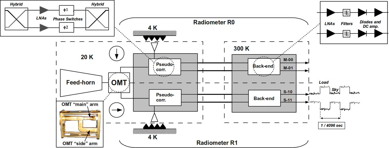
Figure 1 shows a schematic of a complete RCA. The feed horn is connected to an OMT, which splits the incoming radiation into two perpendicular linear polarisation components that propagate through two independent pseudo-correlation differential radiometers. These radiometers are labelled as M or S depending on the arm of the OMT they are connected to (“Main” or “Side”, see lower-left inset of Fig. 1).
In each radiometer, the sky signal coming from the OMT output is continuously compared with a stable 4 K blackbody reference load mounted on the external shield of the HFI 4 K box (Valenziano et al. 2009). After being summed by a first hybrid coupler, the two signals are amplified by dB. A phase shift alternating at 4096 Hz between 0∘ and 180∘ is applied in one of the two amplification chains. A second hybrid coupler separates back the sky and reference load components, which are further amplified and detected in the warm BEU. The output voltage ranges from V to V.
The output diodes are labelled with binary codes 00, 01 (for radiometer M) and 10, 11 (for radiometer S). The four outputs of each radiometric chain are referred to as M-00, M-01, S-10, S-11 (Fig. 1).
After detection, an analog circuit in the data acquisition electronics (DAE) removes a programmable offset to obtain a nearly null DC output voltage, and a programmable gain is applied to match the signal level to the ADC input range.
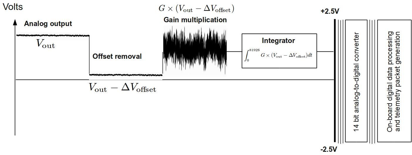
After the ADC, data are downsampled, requantised, compressed according to a scheme described in Herreros et al. (2009) and Maris et al. (2009), and assembled into telemetry packets. On the ground, telemetry packets are converted to volts, using the applied offset and gain factors, and split into sky and reference load time-ordered data (TOD).
2.2 Signal model
In the ideal case of a perflectly balanced radiometer, the differential power output for each of the four diodes can be written as follows (Seiffert et al. 2002; Mennella et al. 2003; Bersanelli et al. 2010):
| (1) |
where is the total gain, is the Boltzmann constant, is the bandwidth, and is the diode constant. and are the sky and reference load antenna temperatures at the inputs of the first hybrid, and is the receiver noise temperature. In this section we always refer to average quantities. We omit, for simplicity, angled brackets, i.e., , , etc.
The gain modulation factor, , is defined by
| (2) |
and is used to balance (in software) the temperature offset between the sky and reference load signals and minimise the residual 1/ noise in the differential datastream. In nominal operating conditions, the gain modulation factor is in the range , depending on channel. This parameter is calculated each pointing period333A pointing period is the amount of time during which the Planck telescope scans the same ring in the sky. from the average uncalibrated total power data using the relationship:
| (3) |
Details about the gain modulation factor calculation and its implementation in the scientific pipeline can be found in Mennella et al. (2003) and Zacchei et al. (2011).
The white noise spectral density at the output of each diode is essentially independent of the reference-load absolute temperature and is given by
| (4) |
If the front-end components are not perfectly balanced, then the separation of the sky and reference load signals after the second hybrid is not perfect and the outputs are mixed. First-order deviations in white noise sensitivity from the ideal behaviour are caused mainly by noise temperature and phase-switch amplitude mismatches. Following the notation used in Seiffert et al. (2002), we define , the imbalance in front end noise temperature, and and , the imbalance in signal attenuation in the two states of the phase switch. Equation 4 for the two diodes of a slightly imbalanced radiometer then becomes
| (5) |
which is identical for the two diodes apart from the sign of the term , representing the phase switch amplitude imbalance. This indicates that the isolation loss caused by this imbalance generates an anticorrelation between the white noise levels of the single-diode data streams.
For this reason, the LFI scientific data streams are obtained by averaging the voltage outputs from the two diodes in each radiometer:
| (6) |
where and are inverse-variance weights calculated from the data as discussed in Zacchei et al. (2011). This way, the diode-diode anti-correlation is cancelled, and the radiometer white noise becomes
| (7) |
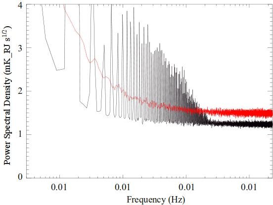
Figure 3 illustrates this anti-correlated noise for a representative LFI channel (LFI28M). In black we plot the amplitude spectral density (ASD) of the weighted sum of the diode pair corresponding to the radiometer. The sky signal is visible as a series of spikes at the satellite rotation frequency and harmonics. The 1/ and white noise levels are clearly visible, too. In red we show the ASD of the weighted difference of the same two diodes, a case in which (as expected) the sky signal is removed. In the difference signal the white noise is nearly 20% higher because of the anti-correlated noise in the output of two diodes. In fact, if the diodes were uncorrelated then the sum and difference of their ASD’s should show identical white noise levels.
While the effects of this correlated component and the proper propagation through the pipeline to maps could be calculated and corrected at the map level, we have found it more natural and effective to combine the diodes in the time domain, performing calibration and further processing on the combined time stream.
2.3 In-band response and centre frequency
The in-band receiver response has been thoroughly modelled and measured for all the LFI detectors during ground tests. The complete set of bandpass curves has been published in Zonca et al. (2009). From each curve we have derived the effective centre frequency according to
| (9) |
where is the receiver bandwidth and is the bandpass response. Table 1 gives the centre frequencies of the 22 LFI radiometers. For each radiometer, is calculated by weight-averaging the bandpass response of the two individual diodes with the same weights used to average detector timestreams. For simplicity and for historical reasons, we will continue to refer to the three channels as the 30, 44, and 70 GHz channels.
|
||||||||||||||||||||||||||||||||||||||||||||||||||||||||||||||
Colour corrections, , needed to derive the brightness temperature of a source with a power-law spectral index , are given in Table 2. The values are averaged for the 11 RCAs and for the three frequency channels. Details about the definition of colour corrections are provided in Zacchei et al. (2011).
| Spectral Index RCA 0.00 1.00 2.00 3.00 4.00 LFI18. 1.054 1.028 1.011 1.003 1.003 1.010 1.026 LFI19. 1.170 1.113 1.066 1.026 0.994 0.969 0.949 LFI20. 1.122 1.079 1.044 1.017 0.997 0.983 0.975 LFI21. 1.087 1.053 1.028 1.010 1.000 0.996 0.998 LFI22. 0.973 0.971 0.976 0.988 1.007 1.033 1.066 LFI23. 1.015 1.004 0.999 0.998 1.003 1.012 1.026 70 GHz average. 1.070 1.041 1.021 1.007 1.001 1.001 1.007 LFI24. 1.028 1.015 1.007 1.002 1.000 1.003 1.009 LFI25. 1.039 1.024 1.013 1.005 1.000 0.999 1.000 LFI26. 1.050 1.032 1.017 1.007 1.000 0.997 0.997 44 GHz average. 1.039 1.024 1.012 1.004 1.000 0.999 1.002 LFI27. 1.078 1.049 1.026 1.010 1.000 0.996 0.998 LFI28. 1.079 1.049 1.026 1.009 1.000 0.997 1.002 30 GHz average. 1.079 1.049 1.026 1.010 1.000 0.997 1.000 |
3 LFI operations
3.1 Cooldown and tuning
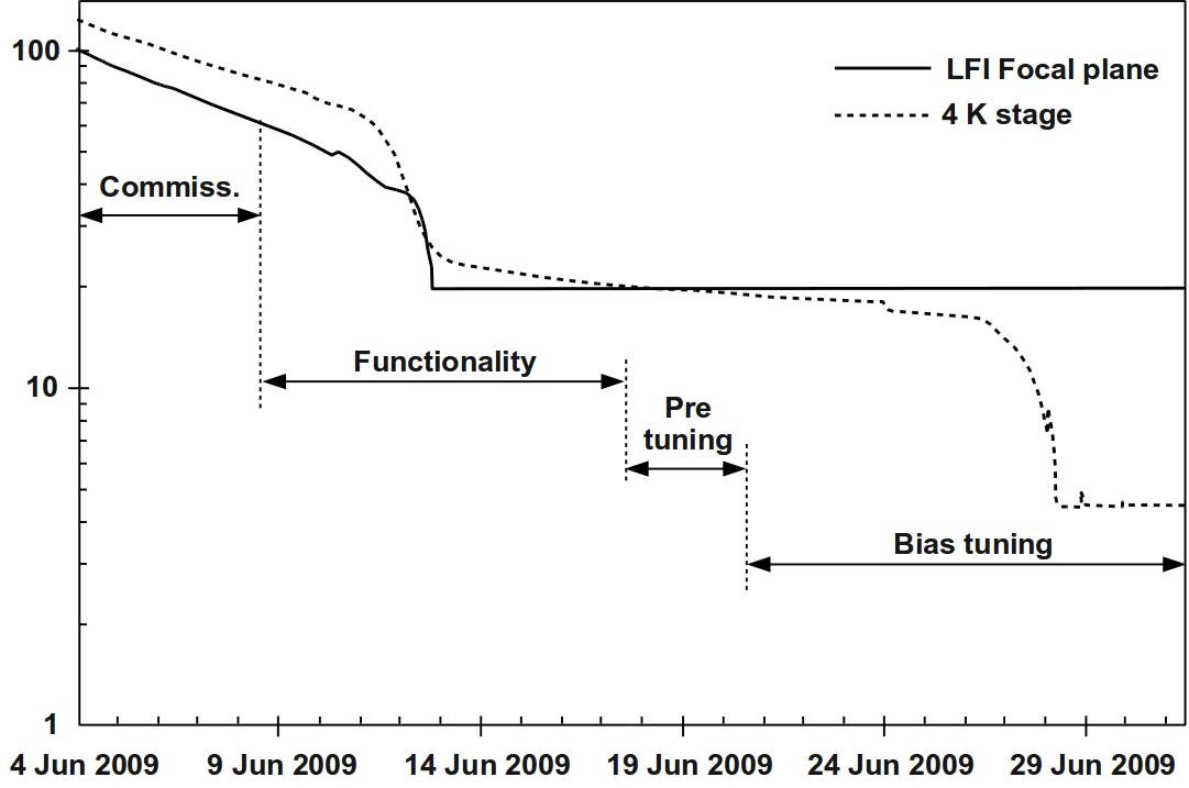
LFI operations began during the calibration, performance, and verification (CPV) phase of the mission. Functionality and tuning tests (Gregorio et al. 2011) were carried out, taking advantage of the varying temperature of the 4K-stage during cooldown (see Fig. 4).
For optimal scientific performance, the bias voltages of the front-end low noise amplifiers (LNAs) and phase switch currents must be carefully tuned. Although radiometer tuning was performed during ground tests (Cuttaia et al. 2009), the procedure was repeated in flight to account for possible changes in the electrical and thermal environment.
Phase switch bias currents (, ) of the 30 GHz and 44 GHz RCAs were tuned to optimise amplitude balance. This was done by exploring a two-dimensional bias surface around the optimal points found during ground tests. The results (repeated also at the end of the tuning campaign) confirmed the optimal points found before launch. The phase switches of the 70 GHz RCAs, instead, were set to the maximum biases (1 mA) and were not tuned. Ground tests showed that the rise time was sensitive to bias currents, and decreased as the current increased from 0.5 mA to 1 mA (Gregorio et al. 2011).
LNA biases were tuned by exploring a large volume in the bias space of each amplifier. The common drain voltage, , the gate voltage of the first stage, , and the gate voltage common to the remaining stages, , were sampled according to a “hyper matrix” (HYM) tuning strategy, in which several bias quadruplets were varied for each radiometer. This strategy increased considerably the sampled parameter space with respect to ground tuning tests (Cuttaia et al. 2009), and allowed us to fully characterise the radiometer performance in terms of noise temperature, isolation, and drain current balance.
To define the broad bias regions to be deeply sampled by the HYM tuning procedure, a pre-tuning phase was run with the instrument at 20 K and the reference loads at 20.4 K. The large imbalance between the sky and reference load signals provided us with enough voltage difference to estimate noise temperature.
During the HYM tuning phase, smaller bias volumes around the optimal pre-tuning points were sampled at four different temperatures (see Fig. 4) between 19.1 K and 4 K during the cooldown of the 4He-JT cooler, allowing us also to characterize the response linearity (Mennella et al. 2009). Drain voltages were also tuned for a limited subset of quadruplets, making the overall bias space six-dimensional.
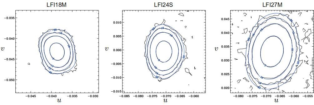
Figure 5 shows an example of “condensed noise temperature” maps. These are contour plots in the space for the LNAs of a given radiometer. Each point in the plot is the average of the best 20% noise temperature values determined by the quadruplets sharing that particular pair. The same approach was used to map isolation and drain currents.
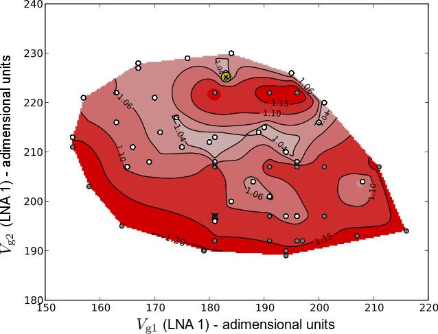
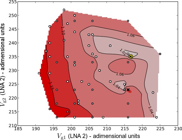
Noise temperature and isolation maps were calculated by fitting data using both a linear and a non-linear response model. Minor effects caused by non-linear response were observed, as expected, only for 30 and 44 GHz channels, confirming on-ground test results. As emphasized in Mennella et al. (2009), signal compression in 30 and 44 GHz receivers is relevant only if the input range is of the order of K. Therefore it can be completely neglected in normal operations and in flight calibration, where the sky dynamic range is mK. The optimal bias values found during tuning were close to those found during satellite-level tests on the ground, with maximum deviations of about 10%. Table 3 summarizes the improvements in noise temperature and isolation between the ground and flight tests.
| Min Median Max [%] [%] [%] . 0 4.2 12.5 . 1 6 115 |
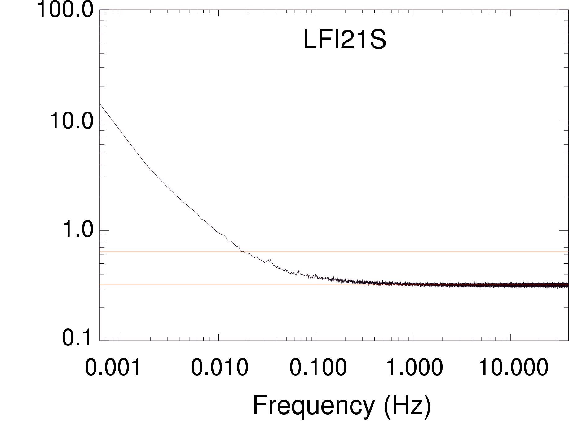
The only large change was in radiometer LFI21S, for which isolation improved from dB measured on ground to dB measured in flight. There was a corresponding improvement in white noise sensitivity (see Sect. 6.2).
After tuning, an unexpectedly high level of noise fluctuations was observed for the 44 GHz RCAs, using either the new flight bias settings or the old ground ones. Dedicated tests showed that this instability was correlated with the phase switch configuration of 70 GHz LFI23, and disappeared when the radiometers were biased with the optimal voltages found during the optimisation of the individual front-end modules before instrument integration (see Fig. 6). This interaction between RCAs belonging to different frequency channels was unexpected and deeply investigated during CPV. The root cause was never fully established, but the most likely explanation was a parasitic oscillation triggered by unexpected cross-talk in the warm electronics. Details about investigations performed in flight to understand and solve this problem are reported in Gregorio et al. (2011). The final bias setting (Davis et al. 2009), characterised by a slightly higher power consumption ( mW) but similar noise and isolation performance, eliminated the problem.
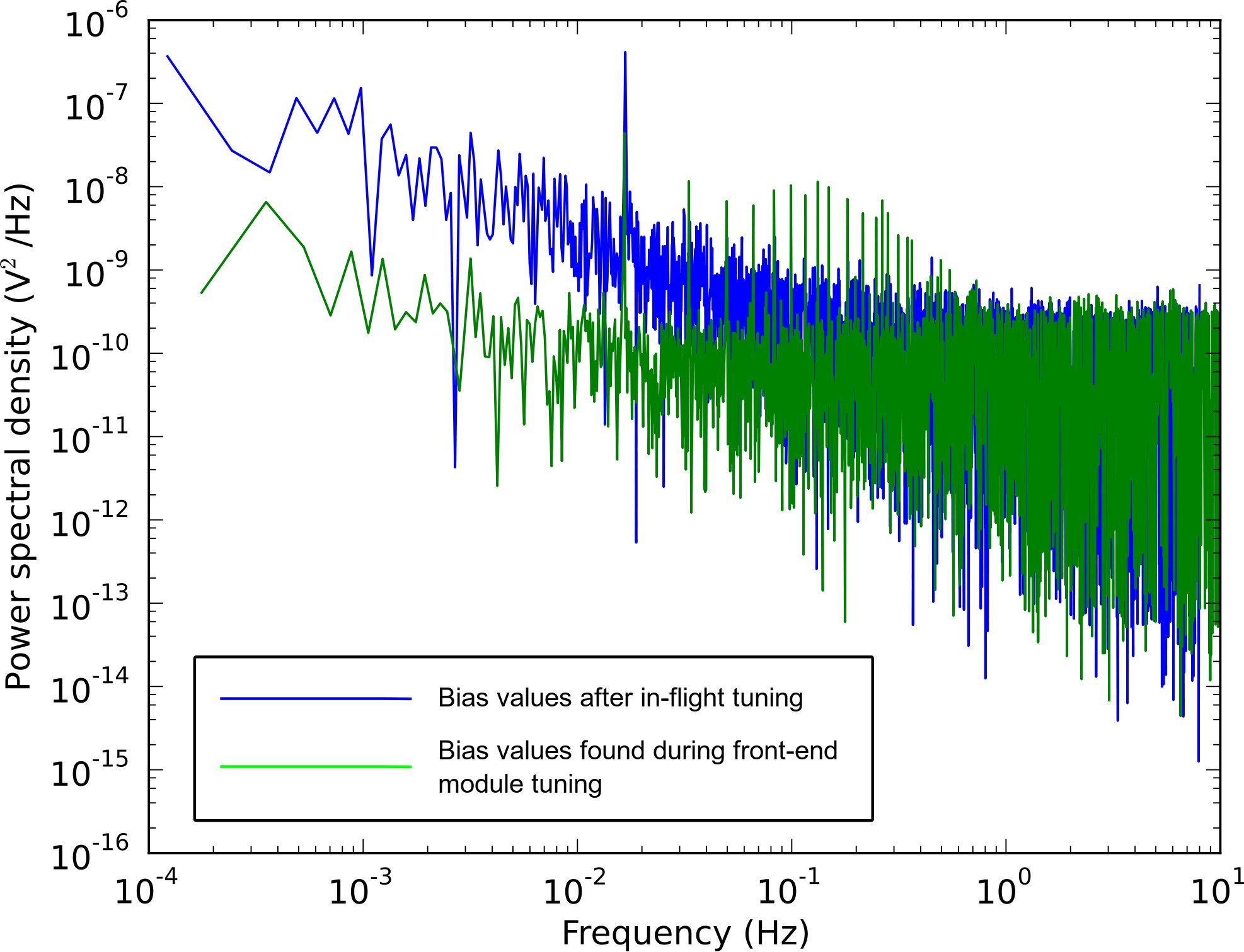
Table 4 summarises the bias settings chosen for the front-end amplifiers at the end of CPV. They have never been changed since the start of nominal operations.
| Radiometer RCA M S LFI18. Flighta Flight LFI19. Groundb Ground LFI20. Ground Ground LFI21. Ground Flight LFI22. Ground Ground LFI23. Ground Ground LFI24. FEMc FEM LFI25. FEM FEM LFI26. FEM FEM LFI27. Ground Ground LFI28. Ground Ground |
| aDetermined during in-flight tests. |
| bDetermined during satellite-level ground tests. |
| cDetermined during module-level ground tests. |
The last tuning step of the CPV phase configures the signal processing unit (SPU) data compressor for each of the 44 LFI channels (Maris et al. 2009) so that the data fit into the allocated telemetry bandwidth without significant loss of sensitivity (defined below) from quantisation errors produced by the lossy compressor. Quantisation errors appear as an additional white noise component that can be characterised as the ratio of the quantisation rms over the intrinsic rms of the signal before compression. The ratio can be monitored directly in-flight with the so-called “calibration channel”, a telemetry mode that provides 15 min of uncompressed data for each diode every day (Bersanelli et al. 2010).
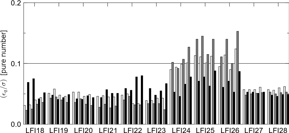
To limit the loss of sensitivity to less than 1%, we require in the differenced data (Maris et al. 2009). The results of the SPU calibration are summarized in Fig. 7 and Table 5. The requirement in the differenced data is satisfied by every channel.
|
||||||||||||||||||||||||||||||||||||||||||||||||||||||||||||||||||||
The stability of the SPU compressor is monitored daily by an automatic procedure that checks for variations of the telemetry and quantisation error and for near-saturation conditions. has changed little during the first year of operations. Typical variations are much less than 1%, with maximum variations around 1.7%.
3.2 Instrument response during cooldown
LFI observations began during the cooldown, even before tuning. Figure 8 shows some of the first differential, uncalibrated output from LFI28M-00.
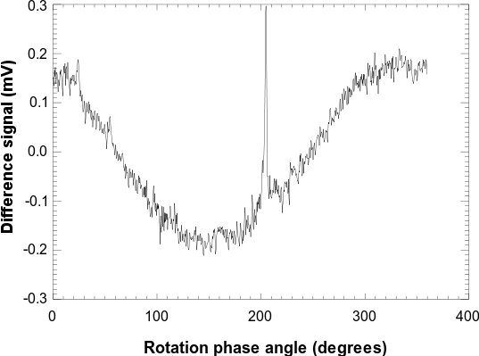
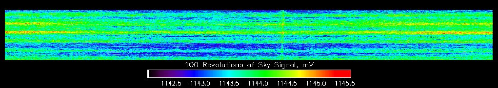
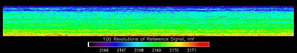
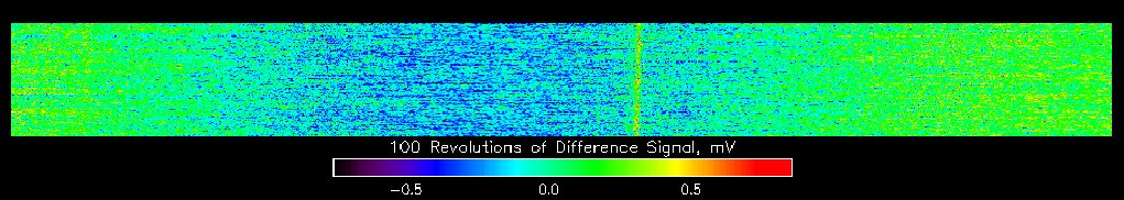
Figure 9 shows a “pseudo-map.” The horizontal axis is spin axis phase angle, the vertical axis is revolution number, and the color scale gives signal amplitude. The map shows the sky, reference, and difference data for 100 telescope revolutions on 14 June 2009. These are the same data that appear in the phase binned map in Fig. 8. In the sky signal, one can see the galaxy spike, a hint of the CMB dipole, and fluctuations slower than the pointing period given by noise fluctuations in the total power voltage output. In the reference load signal, one can see a significant gradient due to the rapid cooldown of the 4 K stage during this period, as well as the same fluctuations seen in the sky signal. In the difference signal, one can see that correlated fluctuations in the sky and reference data are cancelled. The mean value has been subtracted from each revolution in the difference map.
3.3 Operations after verification phase
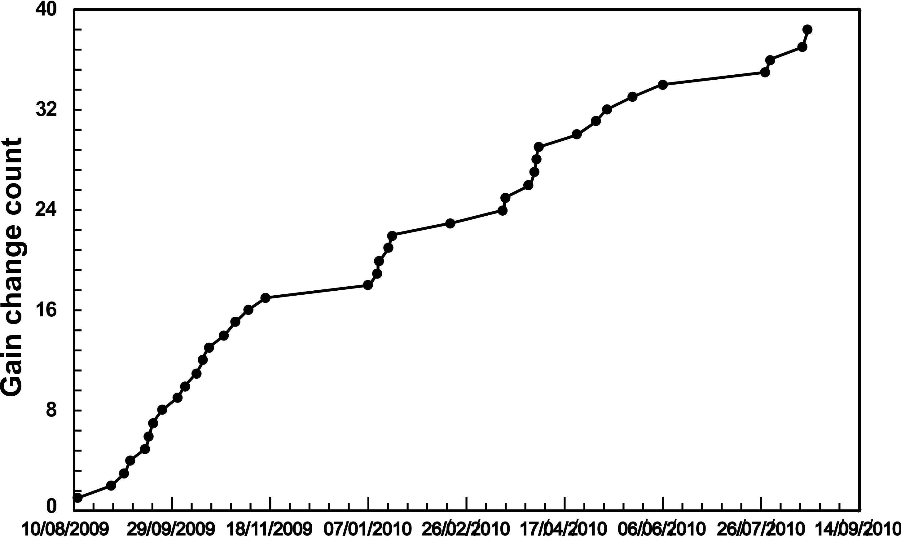
Since the beginning of nominal LFI operations, no instrument parameters have been changed, with one exception. Starting on 11 August 2009, occasional uncommanded jumps in output signal in a single channel were seen, sometimes causing saturation in the ADC and temporary loss of science data. These jumps were traced to single bit-flip changes in the DAE gain-setting circuit, presumably a result of single-event upsets (SEUs) from cosmic rays. Initially, science data were lost in saturated channels until the gain could be reset during the next downlink period. Starting in October 2009, an automatic procedure resets all gain values every min.
Figure 10 shows the cumulative number of gain change events as a function of time during the first year of operation. A total of 38 were seen through 30 September 2010, corresponding to an average rate of about one event every 11 days. Out of these 38 events, 13 saturated the ADC, leading to lost observation time from the corresponding detector, five did not saturate the ADC but the compression algorithm was not able to deal with the anomalous signal statistics, and 20 could be recovered simply by applying the correct gain after the event.
In most cases the gain increased, but occasionally it decreased. The bit flip occurs in different channels, on different bits, and the resulting value after the flip is not always the same. The most significant bit (controlling the second amplifier stage) never flips, suggesting that the component undergoing a possible single event upset (SEU) is the programmable gain amplifier in the first amplifier stage, an Analog Devices AD526SD/883B. The internal technology of the gain amplifiers in the two stages is different, therefore a different sensitivity to high energy events would not be too surprising. Nevertheless, investigation444Bibliographic research on Electronic Radiation Response Information Center (ERRIC), NASA GFSC Radhome; ESA radiation effect database revealed no information on SEU effects on AD526 devices. The event rate is too low to reveal a correlation between solar activity and cosmic ray fluxes as measured by the onboard space radiation environment monitor (SREM; Planck Collaboration (2011a)); however, a significant population of high energy cosmic rays, larger than expected before launch, has been observed by the HFI instrument (Planck HFI Core Team 2011).
3.4 Missing and usable data
Since the start of the mission, only a small percentage of the LFI science data have been lost or considered unusable for science. Table 6 gives the percentage of time lost to missing data, anomalies, and maneuvers for the period from 12 August 2009 to 7 June 2010.
The main source of missing data is telemetry packets where the arithmetic compression performed by the SPU is incorrect, causing a decompression error. There were 15 such packets in all LFI channels, with negligible scientific impact. For instance, for the entire 70 GHz frequency channel, there are just 101 lost seconds.
Anomalies include the DAE gain jumps described in Sect. 3.3, and other instabilities (see Sect. 5.1) that make the data unsuitable for science.
Spacecraft maneuvers, from routine repointings of the spin axis to stationkeeping maneuvers (see Planck Collaboration (2011a)) cause by far the largest fraction of discarded data so far; however, we expect these data to be fully recovered after additional analysis of the startracker and gyroscope data. If this expectation is met, and the performance of Planck remains as it has been, well over 99% of all observing time will be usable.
|
4 Beams and angular resolution
The most accurate measurements of the LFI main beams have been made with Jupiter, the most powerful unresolved (to Planck) celestial source in the LFI frequency range. Since the LFI feed horns point to different positions on the sky, they detect the signal at different times. Table 7 gives the dates of Jupiter observations in the Fall of 2009.
| RCA Operational Day Date 70 GHz 18, 23. 168–169 28 October–29 October 19, 22. 169–170 29 October–30 October 18, 23. 169–171 29 October–31 October 44 GHz 24. 170–171 30 October–31 October 25, 26. 163–165 23 October–25 October 30 GHz 27, 28. 170–172 30 October–1 November |
The first step in extraction of the beams was to remove -type noise from the data using the Madam destriping map-making code. Planets were masked during this process. Details of the Madam destriper and of the pipeline implemented to extract beams from planet measurements is reported in Zacchei et al. (2011).
To map the beam, each sample contained in the selected timelines was projected in the -plane perpendicular to the nominal line-of-sight (LOS) of the telescope (and at to the satellite spin axis). The and coordinates are defined in terms of the usual spherical coordinates :
| (10) |
To increase the signal-to-noise ratio, data were binned in an angular region of 2′ for the 70 GHz channels and 4′ for the 30 and 44 GHz channels. We recovered all beams down to dB from the peak. An elliptical Gaussian was fit to each beam for both M and S radiometers. The FWHM given in Table 8 is the square root of the product of the major axis and minor axis FWHMs of the individual beams, averaged between M and S radiometers. The uncertainties in Table 8 are the standard deviation of the mean of the statistical uncertainties of the fit. Although a small difference between the M and S beams caused by optics and receiver non-idealities can be expected, for the purpose of point-source extraction relevant for this paper the beams have been considered identical, as this effect is well within the statistical uncertainty.
The ellipticity and orientation of the beams are fundamental parameters. Exhaustive results and details on the determination of all LFI beam parameters will be presented in the future. For the purpose of this paper, Table 8 gives the typical FWHM and ellipticity averaged over each frequency channel.
Figure 11 shows three examples of measured beams compared with calculations performed with the GRASP9555http://www.ticra.com software. The calculated beams have been smeared appropriately to take into account satellite rotation and sampling. The effect of sampling is evident already at dB and cannot be neglected (the typical effect on FWHM is 2% at 70 GHz). In the comparison of measured and calculated beams, the peak of the simulated beam was aligned with the peak of the measured beam (calculated from a Gaussian elliptical fit). The electromagnetic model of the design telescope (Sandri et al. 2010) was used as a reference in the comparison. Ideal parameters have been assumed for the shape of the mirrors, the alignment of the telescope and focal plane unit, as well as for the pattern of the feed horns. The good agreement down to dB demonstrates that, to first order, the overall LFI optical system is performing as expected. Comparison with a more realistic telescope model, including the actual alignment, measured mirror shapes, and measured feedhorn patterns, will be considered in future work.
| FWHMa Uncertaintyb RCA [′] [′] Ellipticityc 70 GHz average. 13.01 1.27 LFI18 . 13.39 0.170 LFI19 . 13.01 0.174 LFI20 . 12.75 0.170 LFI21 . 12.74 0.156 LFI22 . 12.87 0.164 LFI23 . 13.27 0.171 44 GHz average. 27.92 1.26 LFI24. 22.98 0.652 LFI25. 30.46 1.075 LFI26. 30.31 1.131 30 GHz average. 32.65 1.38 LFI27. 32.65 1.266 LFI28. 32.66 1.287 |
| aThe square root of the product of the major axis and minor axis FWHMs of the individual RCA beams, averaged between M and S radiometers. |
| bThe standard deviation of the mean of the statistical uncertainties of the fit. Although a small difference between the M and S beams caused by optics and receiver non-idealities can be expected, for the purpose of point-source extraction relevant for this paper the beams are considered identical, as this effect is well within the statistical uncertainty. |
| cRatio of the major and minor axes of the fitted elliptical Gaussian. |
5 Stability and calibration
5.1 Stability
Thanks to its differential scheme, the LFI is insensitive to many effects in the total-power data caused by noise, thermal fluctuations, or electrical instabilities.
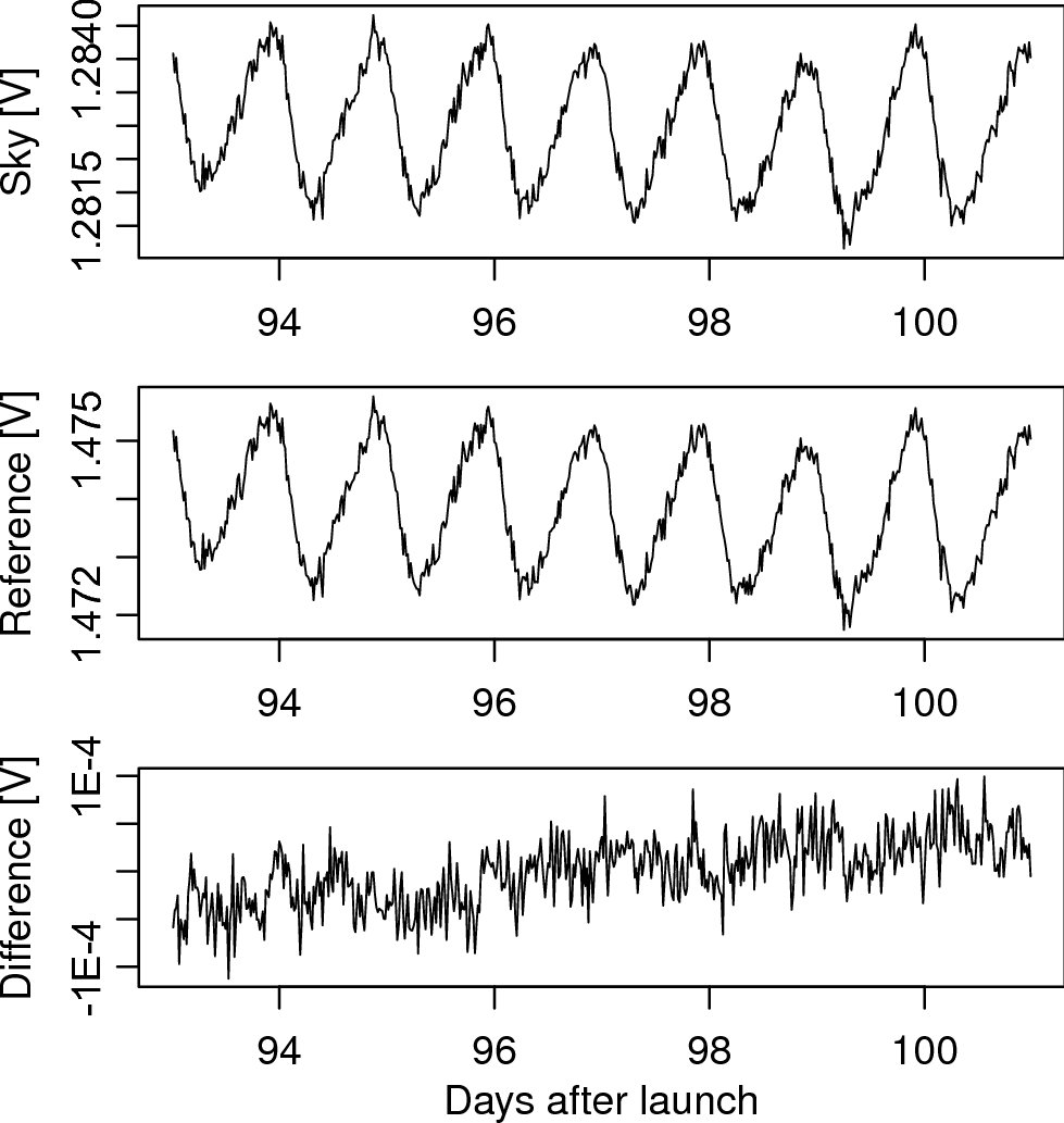
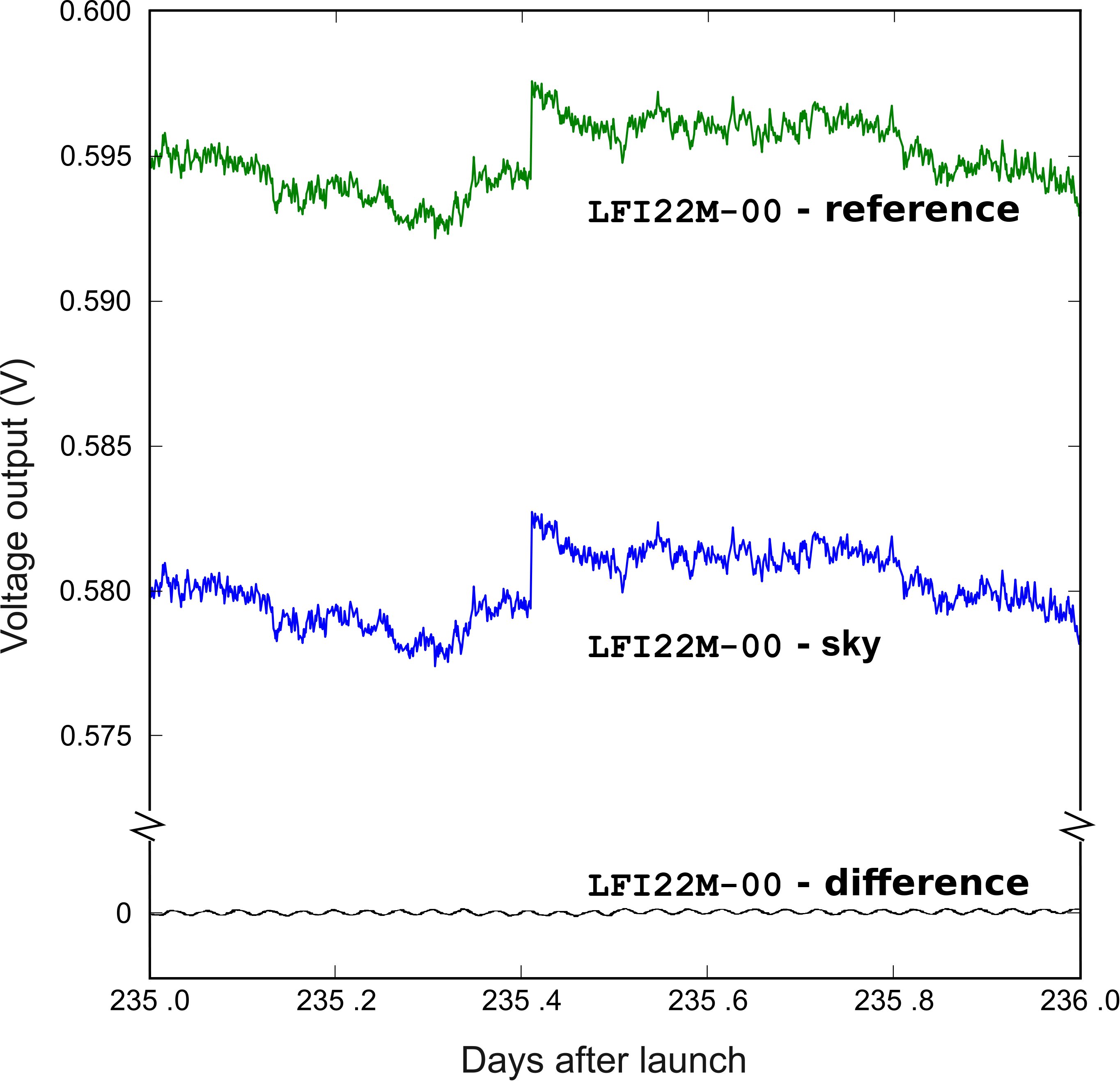
One effect detected during the first survey was the daily temperature fluctuation in the back-end unit induced by the transponder, which was turned on only for downlinks for the first 258 days of the mission (Planck Collaboration 2011b, §§ 2.4.1 and 5.1). Fig. 12 shows the effect of these fluctuations on the radiometeric output of LFI27M. As expected, the effect is highly correlated between the sky and reference load signals. In the difference, the variation is reduced by a factor , where is the gain modulation factor defined in Eq. (3).
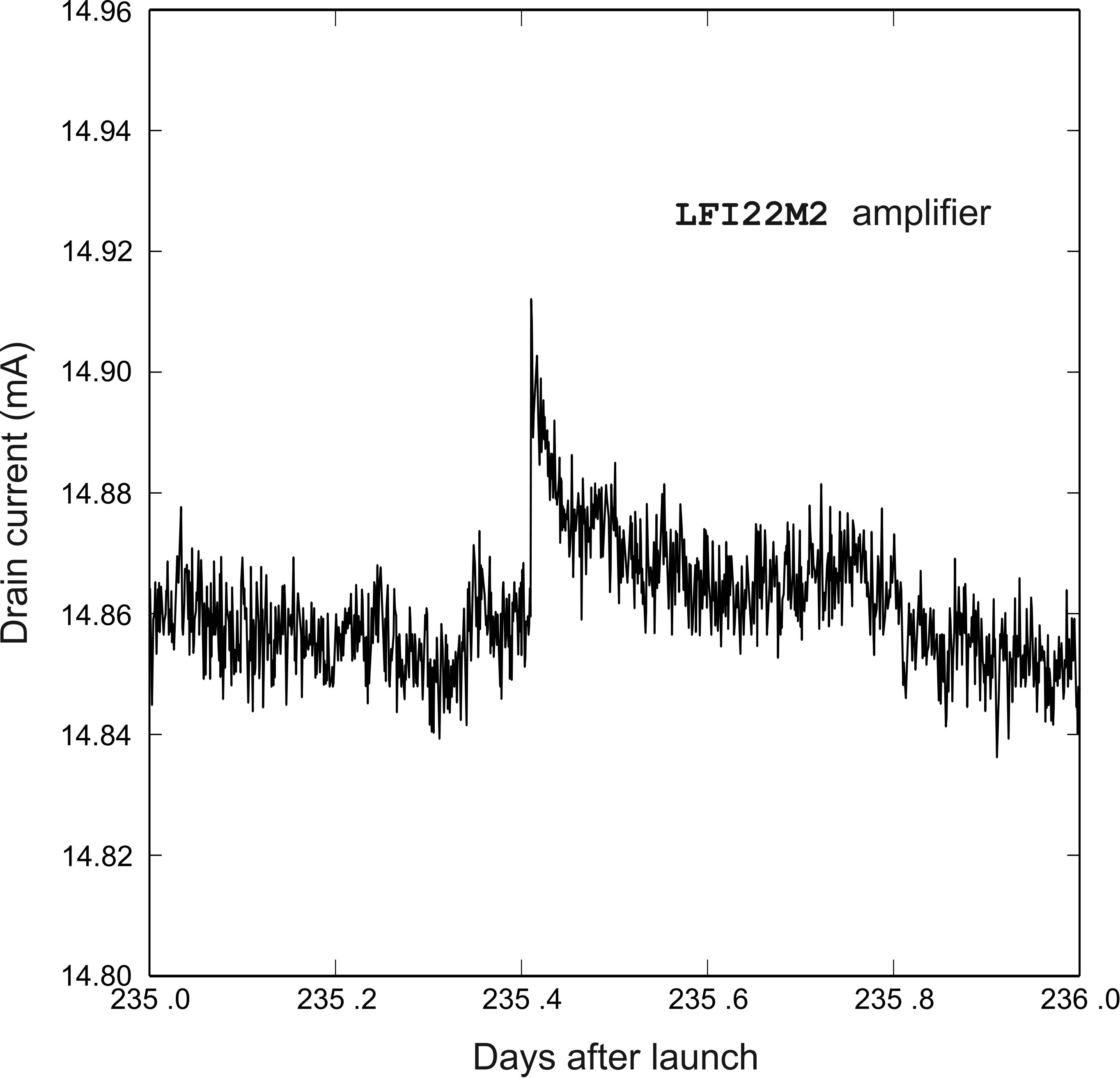
A particular class of signal fluctuations occasionally observed during operations is represented by electrical instabilities that appear as abrupt increases in the measured drain current of the front-end amplifiers with a variable relaxation time from few seconds to some hundreds of seconds. Typically, these events cause a change in both sky and reference load signals and disappear in the difference (see Fig. 13).
Because these effects are essentially common-mode, their residual on the differenced data is negligible, and the data are suitable for science production. In a few cases the residual fluctuation in the differential output was large enough (a few millikelvin in calibrated antenna temperature units) to be flagged, and the data are not used. The total amount of discarded data for all LFI channels until Operational Day 389 was about 2000 s per detector, or 0.008%.
 |
 |
A further peculiar effect appeared in the 44 GHz detectors, where single isolated samples, either on the sky or the reference voltage output, were far from the rest. Over a reference period of four months, 15 occurrences of single-sample spikes (out of 24 total anomaly events) were discarded, an insignificant loss of data.
5.2 Calibration
Photometric calibration, i.e., conversion from voltage to antenna temperature, is performed for each radiometer after total power data have been cleaned of 1 Hz frequency spikes (see § 7 and Zacchei et al. (2011)), and differenced.
Our calibrator is the well-known dipole signal induced by Earth and spacecraft motions with respect to the CMB rest frame. The largest calibration uncertainty comes from the presence of the Galaxy and of the CMB anisotropies in the measured signal. We therefore use an iterative calibration procedure in which the dipole is fit and subtracted, producing a sky map that is then subtracted from the original data to enhance the dipole signal for the next iteration. Typically, convergence is obtained after few tens of iterations.
The thin gray line in Fig. 14 shows the result of this iterative process for the radiometer LFI21M, pointing period by pointing period. In the most stable regions the gain values display relative variations of rms and peak-to-peak. In the most unstable region, where the spacecraft spin was nearly aligned with the dipole and the dipole signal was weak, the relative variations are r.m.s. and peak-to-peak. These variations reflect statistical uncertainties in the determination of the gain over a single pointing period, rather than actual changes in gain.
We can put a limit on the true intrinsic gain variations by looking at the variation of the total power voltage output (cf. § 5.1). The small variations in total power constrain intrinsic gain variations to be less than 1%.
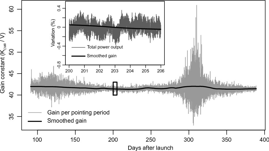
The gain solution based on individual pointing periods was therefore processed to improve its stability by implementing two running averages that have been further smoothed with wavelets: one with a 5-day window, used in the strong dipole regions, and the other with a 30-day window, used in the weak dipole regions. In particular cases, where a true known instrument gain change had to be traced666e.g., when the satellite started using the transponder always “on” which caused a change in the instrument warm unit temperature. we used a 5-day un-smoothed window. In Fig. 14 the the thick black line gives the smoothed gain curve; variations are now rms and peak-to-peak. The inset in the figures compares the smoothed gain and the relative gain variation obtained from Eq. (15), which represent true gain fluctuations in the instrument at the level of . In the current gain model implementation these changes are neglected, but they will be incuded in future versions of our analysis.
5.3 Calibration accuracy
Following COBE and WMAP (Kogut et al. 1996; Jarosik et al. 2011), our main calibrator is the dipole modulation in the CMB. In our current calibration model we use as calibration signal the sum of the solar dipole and the orbital dipole , which is the contribution from Planck orbital velocity around the Sun:
| (11) |
where is the angle between the spacecraft axis and the overall dipole axis (solar + orbital).
In Eq. (11), the absolute calibration uncertainty is dominated by the uncertainty in , which is known only to about 1%. The modulation of the orbital dipole by the Earth’s motion around the Sun is known with an uncertainty almost three orders of magnitude smaller; however, at least one complete Planck orbit is needed for its measurement. In the future, calibration based on the Earth orbital modulation will be significantly more accurate.
The accuracy of our current calibration can be estimated by taking into account two components: 1) the statistical uncertainty in the regions of weak dipole; and 2) the systematic uncertainty caused by neglecting gain fluctuations that occur on periods shorter than the smoothing window. Neglecting the contribution from the wavelet filters and assuming, for simplicity, that the smoothing is done using plain averages, we can write the statistical uncertainty as:
| (12) |
where is the overall number of pointings over the considered period and is the number of pointings for each smoothing region (5 or 30 days).
Table 9 lists the largest statistical uncertainties in four time windows (days 100–140, 280–320, 205–245, 349–389), the first two corresponding to minimum and the second two to maximum dipole response.
|
||||||||||||||||||||||||||||||||||||||||||||||||||
Our current calibration scheme neglects systematic gain variations caused by thermal fluctuations, which introduce spurious signal fluctuations on timescales ranging from 1 to 24 hours. Being much slower than the satellite spin period, these fluctuations are well-removed during map-making by the destriping algorithm (Keihänen et al. 2005, 2010; Zacchei et al. 2011), so that the rms systematic uncertainty per pixel in the final maps due to imperfect calibration is at sub-microkelvin levels (see § 7.2). However, we expect that a more accurate description of the gain variations over short timescales will improve our calibration accuracy even at the level of time ordered data. If we use the dipole signature to estimate an average value for the gain over long time periods (e.g., several months), we can write the gain versus time as
| (13) |
where is the relative gain variation.
The simplest and most direct measurement of gain changes is through the monitoring of the stability of the reference load total power voltage output, , where . The relative output voltage variation is:
If the fractional variations in the noise temperature and in the reference load signal are negligible compared to gain variations, then we have that:
| (15) |
Considering that is in the range 10–30 K and that the reference load temperature is about 4.5 K with fluctuations of mK, we have . Fluctuations in the noise temperature due to thermal changes can be estimated by assuming a coupling of 0.5 K K-1 and taking a typical temperature fluctuation of 1 mK in the front-end unit. We have , which implies that any variation in the total power signal that is larger than is due to actual changes in the gain.
Figure 15 shows two estimates for based on the temperature sensors in the radiometer back-end and on the relative variation of the reference load voltage output (black line).
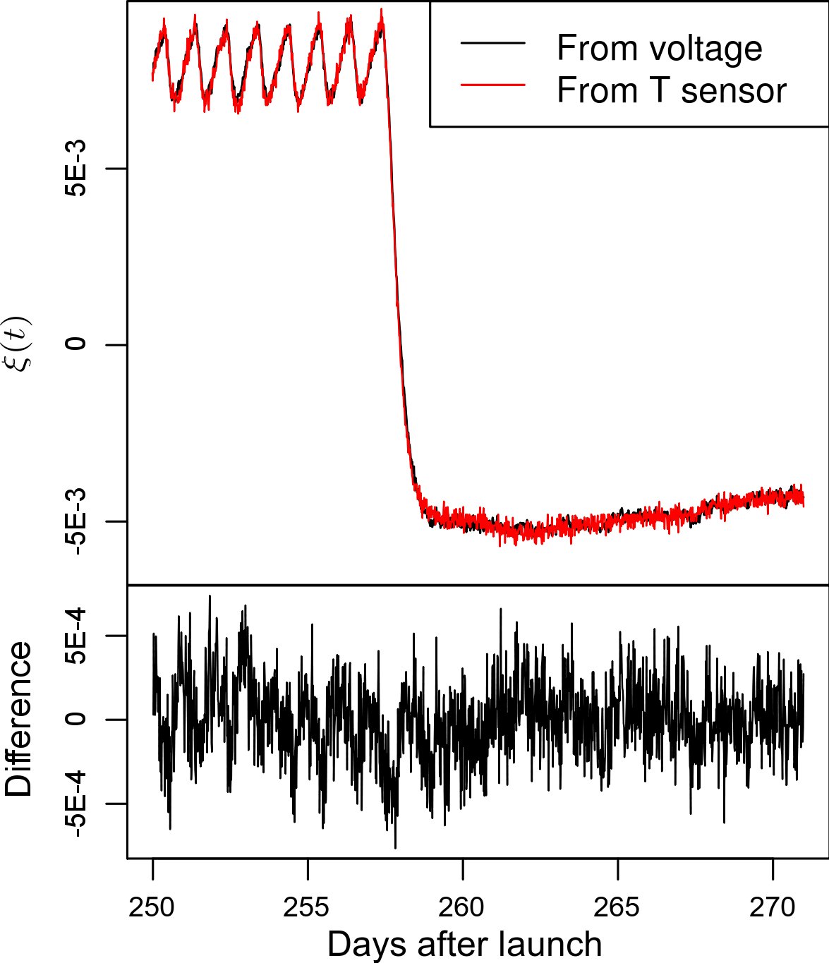
In future versions of the LFI gain model, we plan to use the iterative solution as a starting point and then trace gain changes down to short time scales both by using housekeeping information and by monitoring the relative variation of the total power radiometric output (Eq. (15)).
6 Noise properties
The noise characteristics of the LFI datastreams are closely reproduced by a simple (white + ) noise model:
| (16) |
where is the power spectrum and .
In this model, noise properties are characterised by three parameters, the white noise limit , the knee frequency777The frequency at which the and white noise contribute equally in power. , and the exponent of the component , also referred to as “slope.” In this section we show how the LFI noise has been characterised in flight, and we give noise performace estimates based on one year of operations.
6.1 Method
Noise properties have been calculated following two different and complementary approaches: 1) fitting Eq. (16) to time-ordered data for each radiometer; and 2) building normalised noise maps by differencing data from the first half of the pointing period with data from the second half of the pointing period to remove the sky signal (“jackknife” data sets).
6.1.1 Noise power spectrum estimation in frequency domain
Estimation of noise power spectra from time ordered data is part of the iterative approach in the ROMA map-making suite (Prunet et al. 2001; Natoli et al. 2001; de Gasperis et al. 2005). We produced joint estimates for both signal (i.e., maps) and noise, and then fitted the resulting noise power spectra to Eq. (16) to estimate the three basic noise parameters , , and . All details relative to the pipeline are provided in Zacchei et al. (2011).
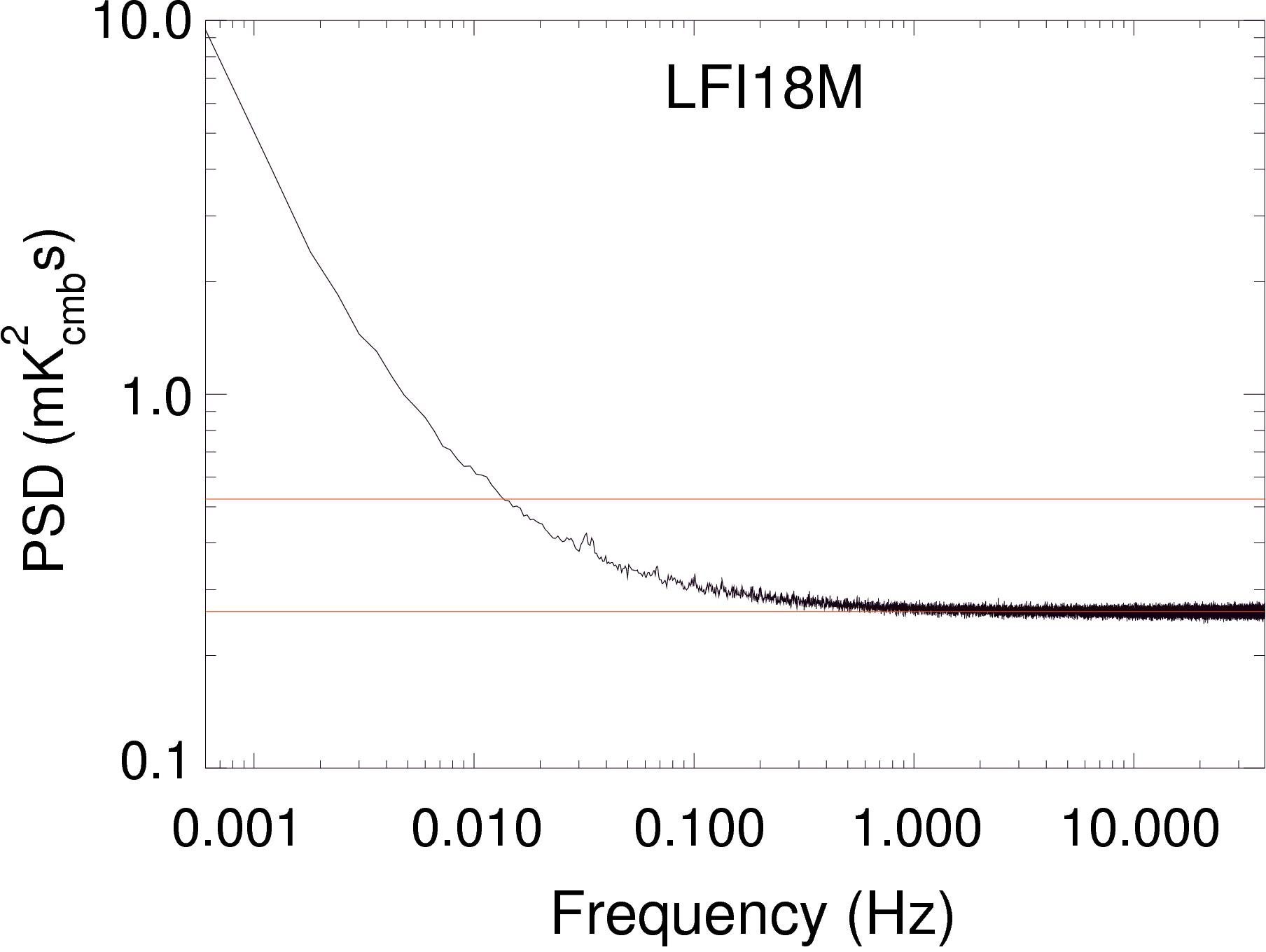
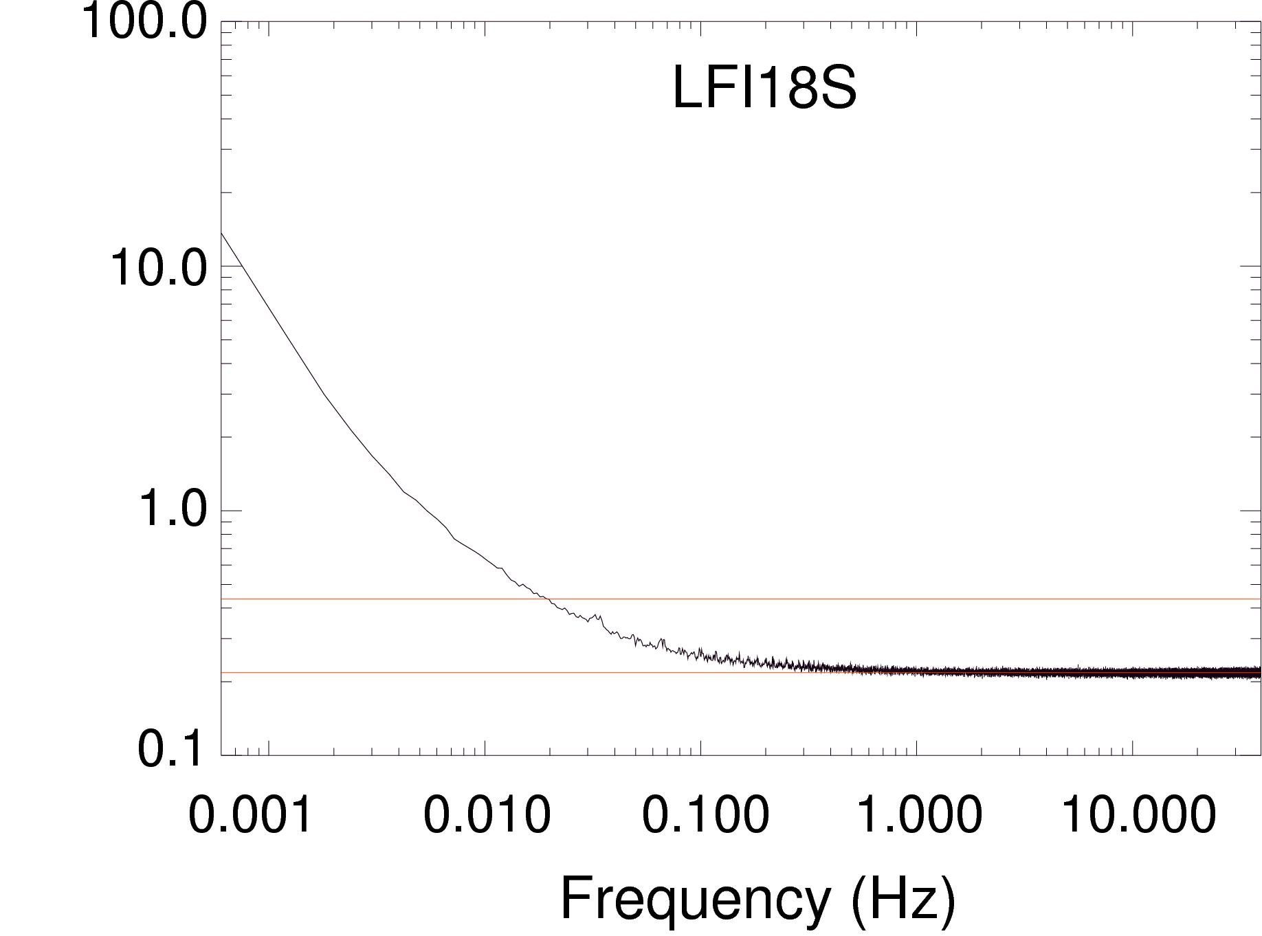
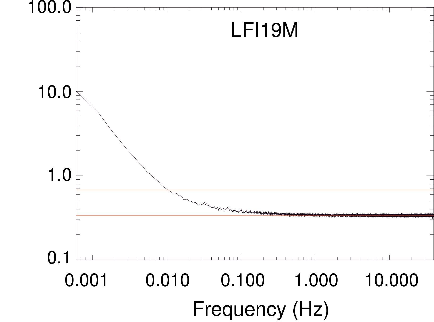
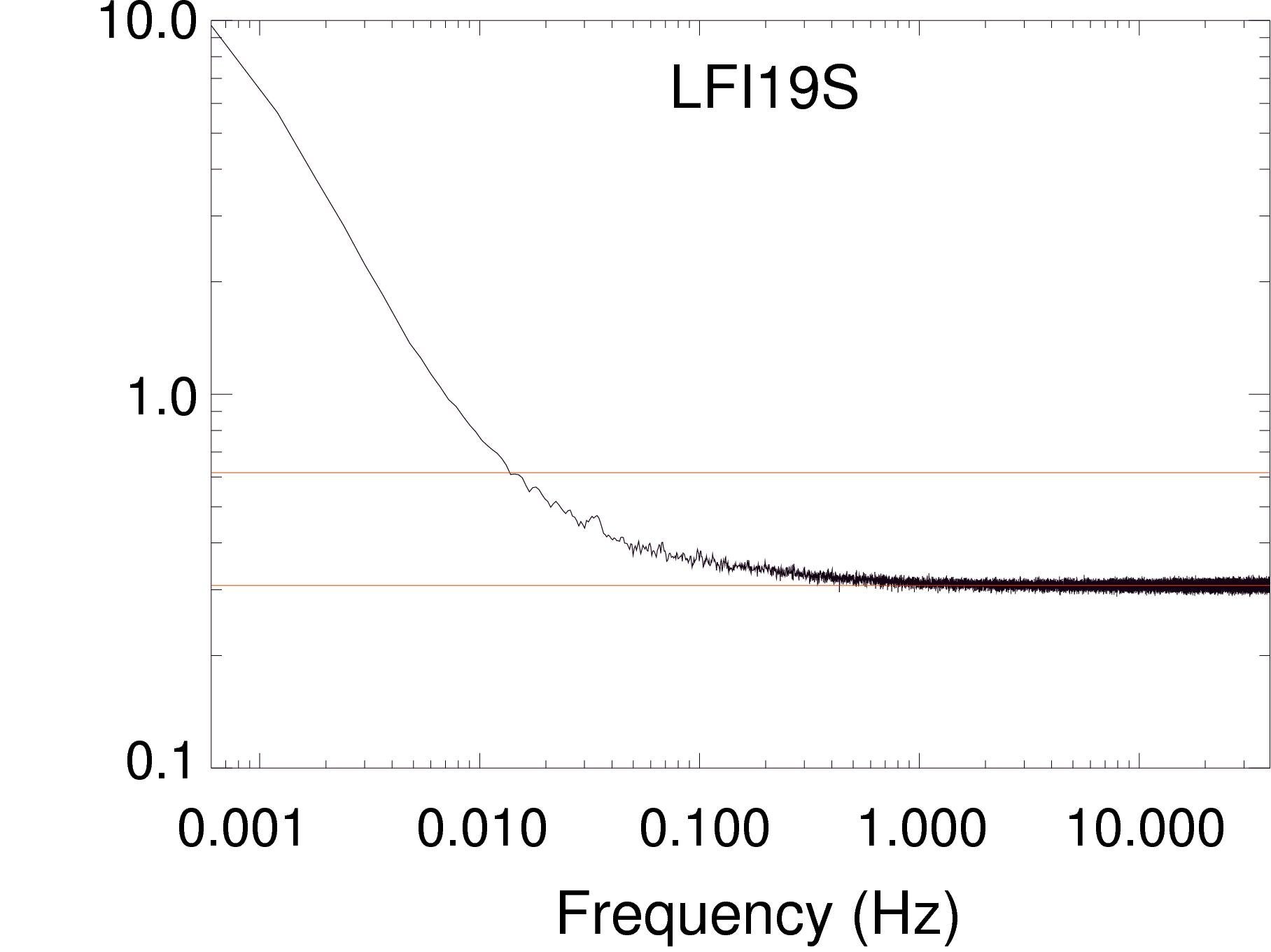
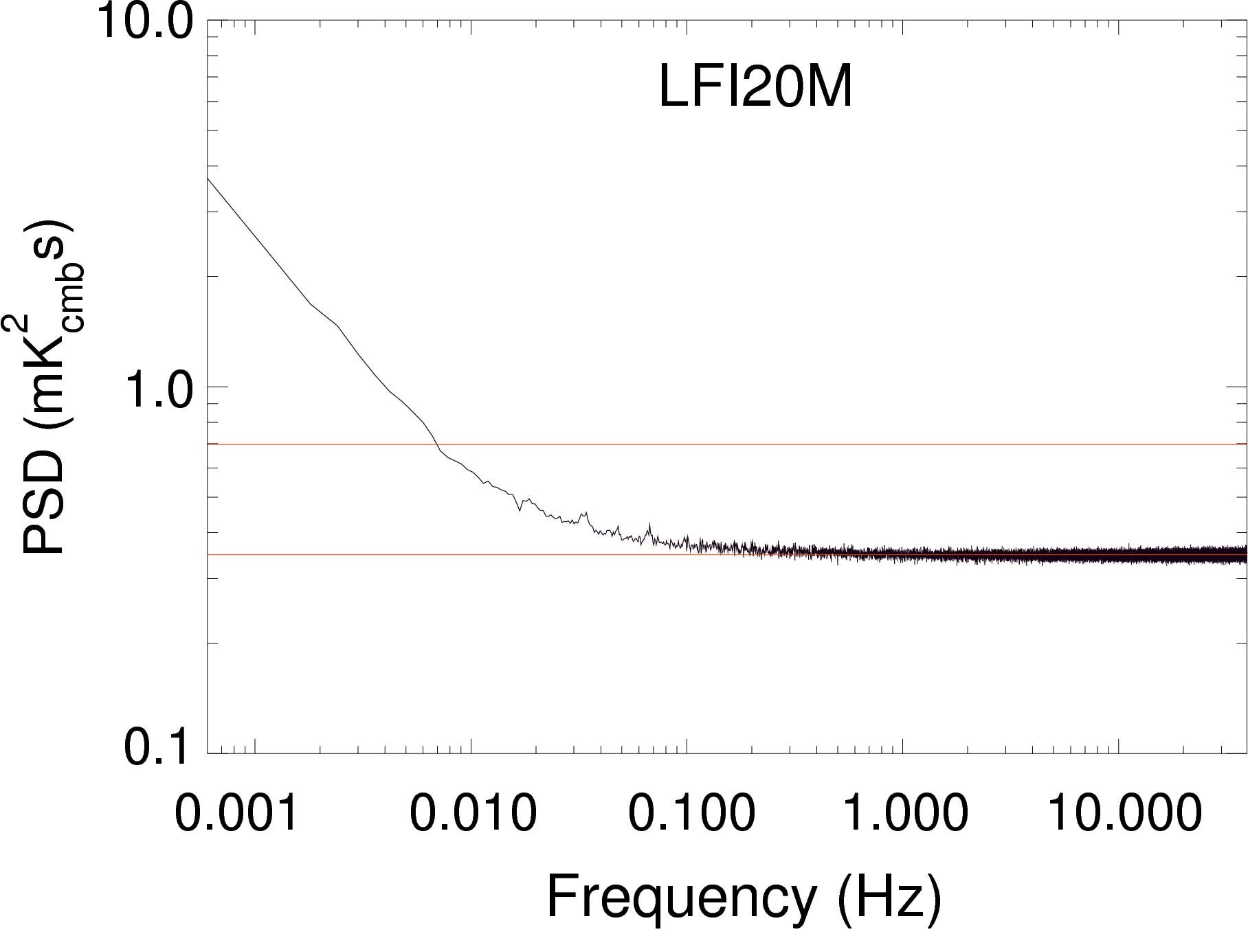
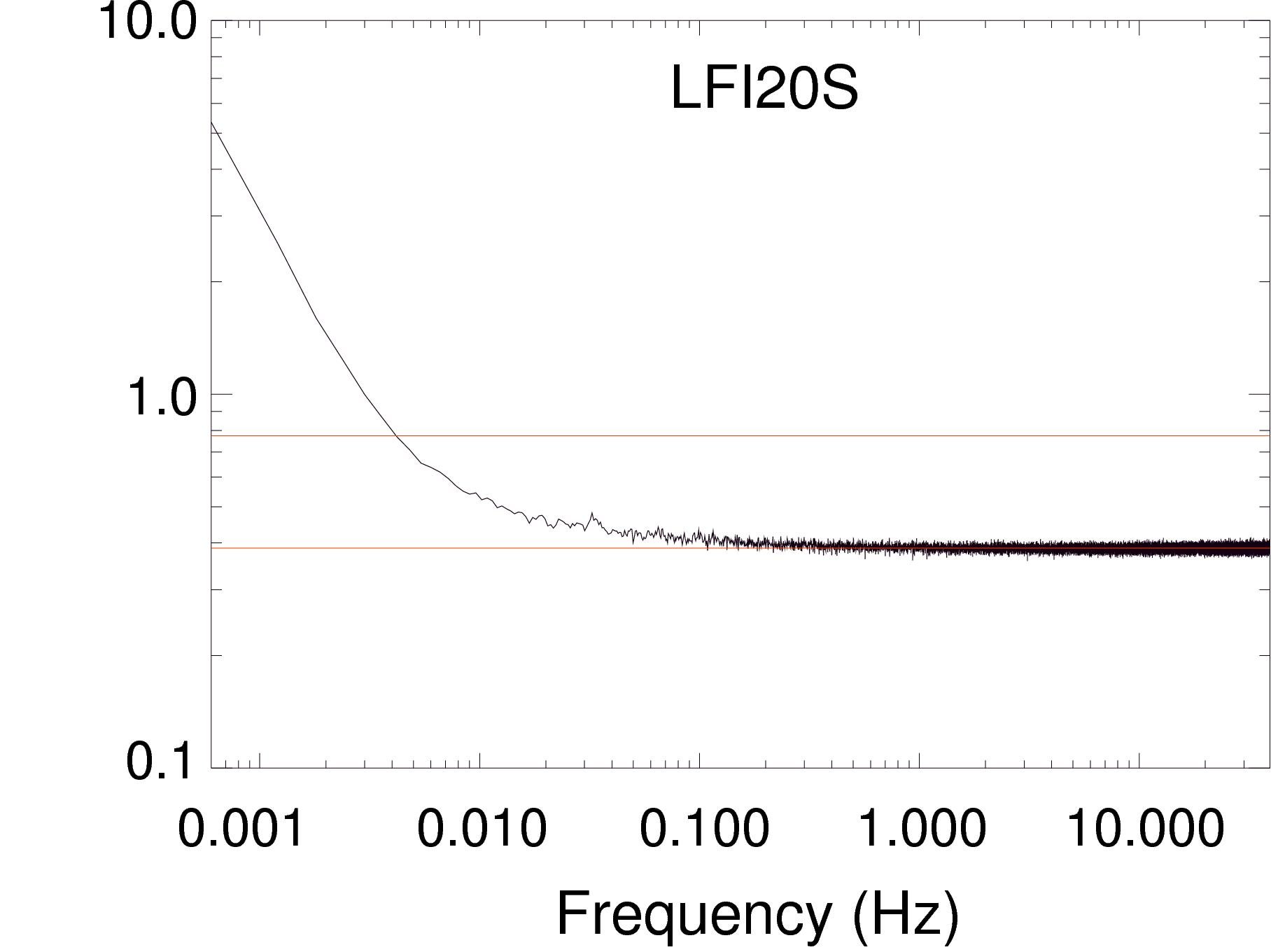
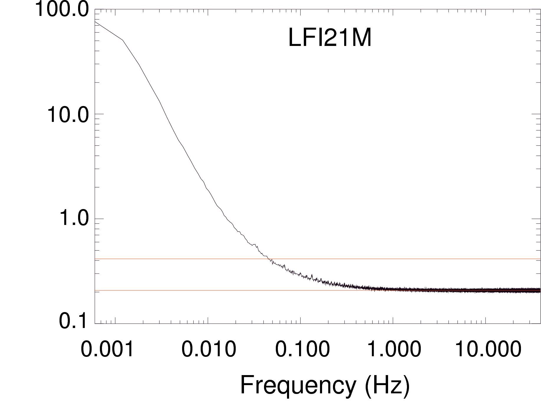
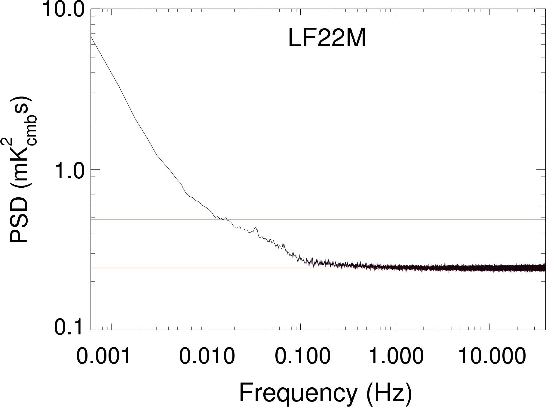
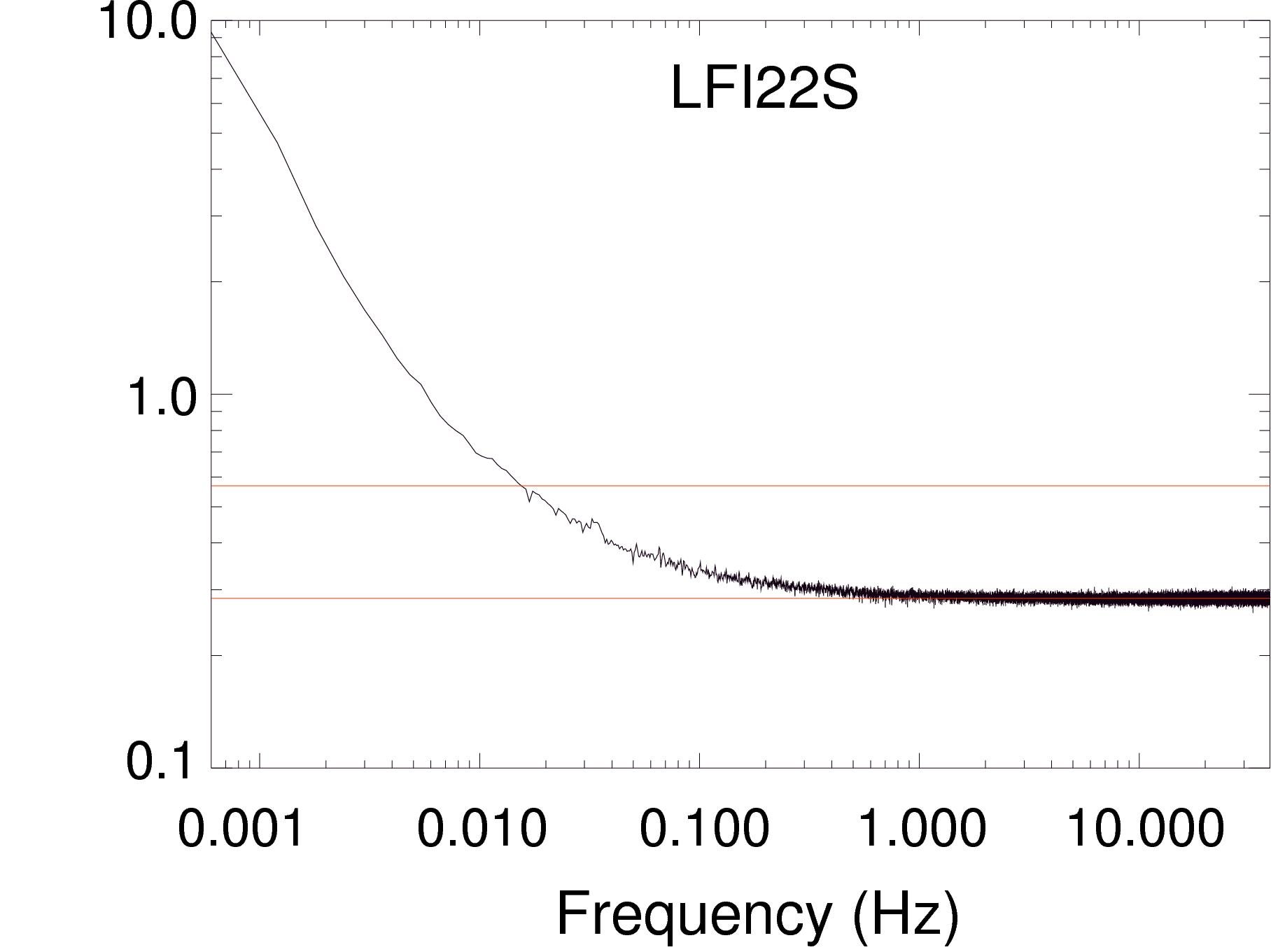
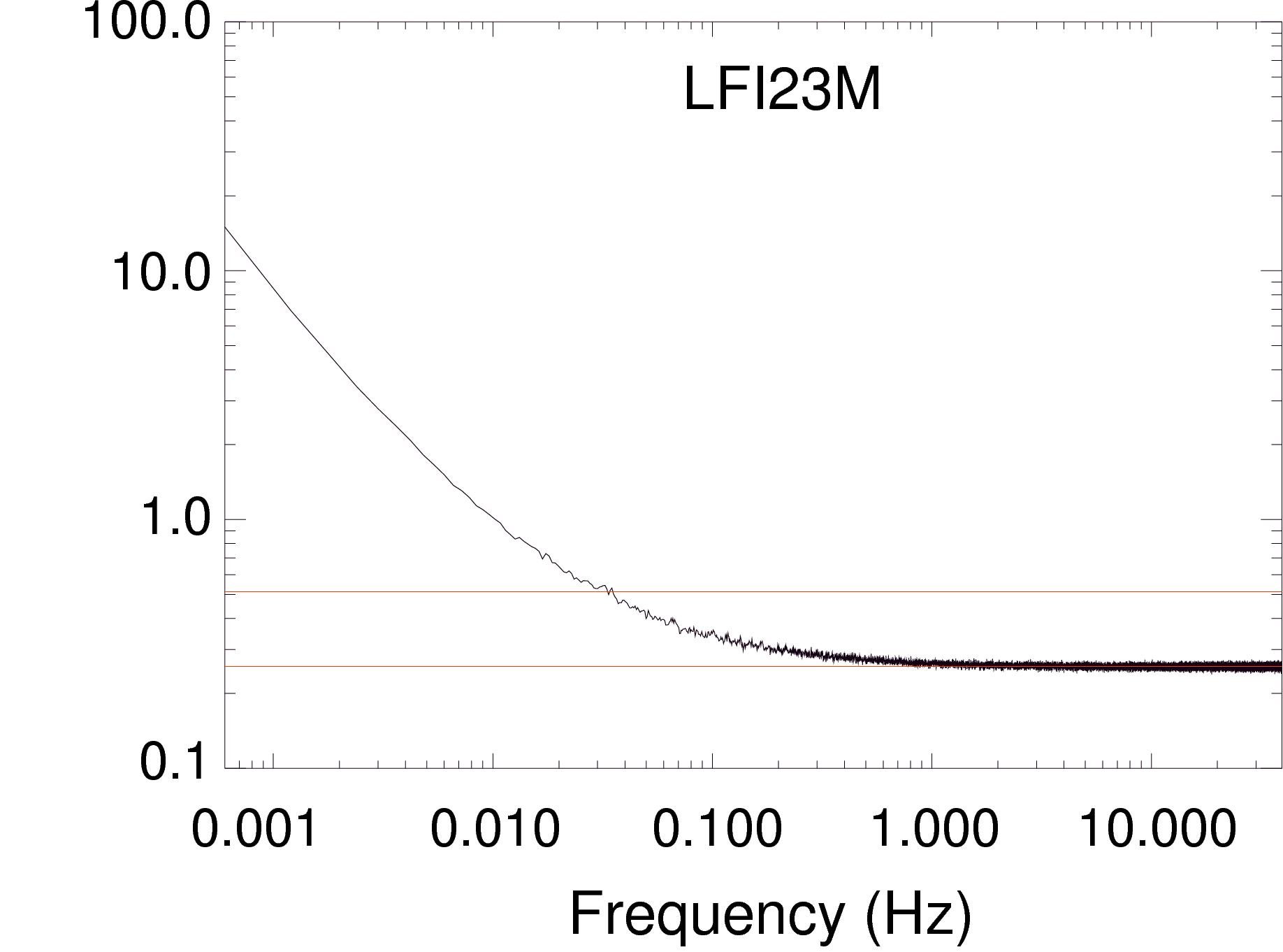
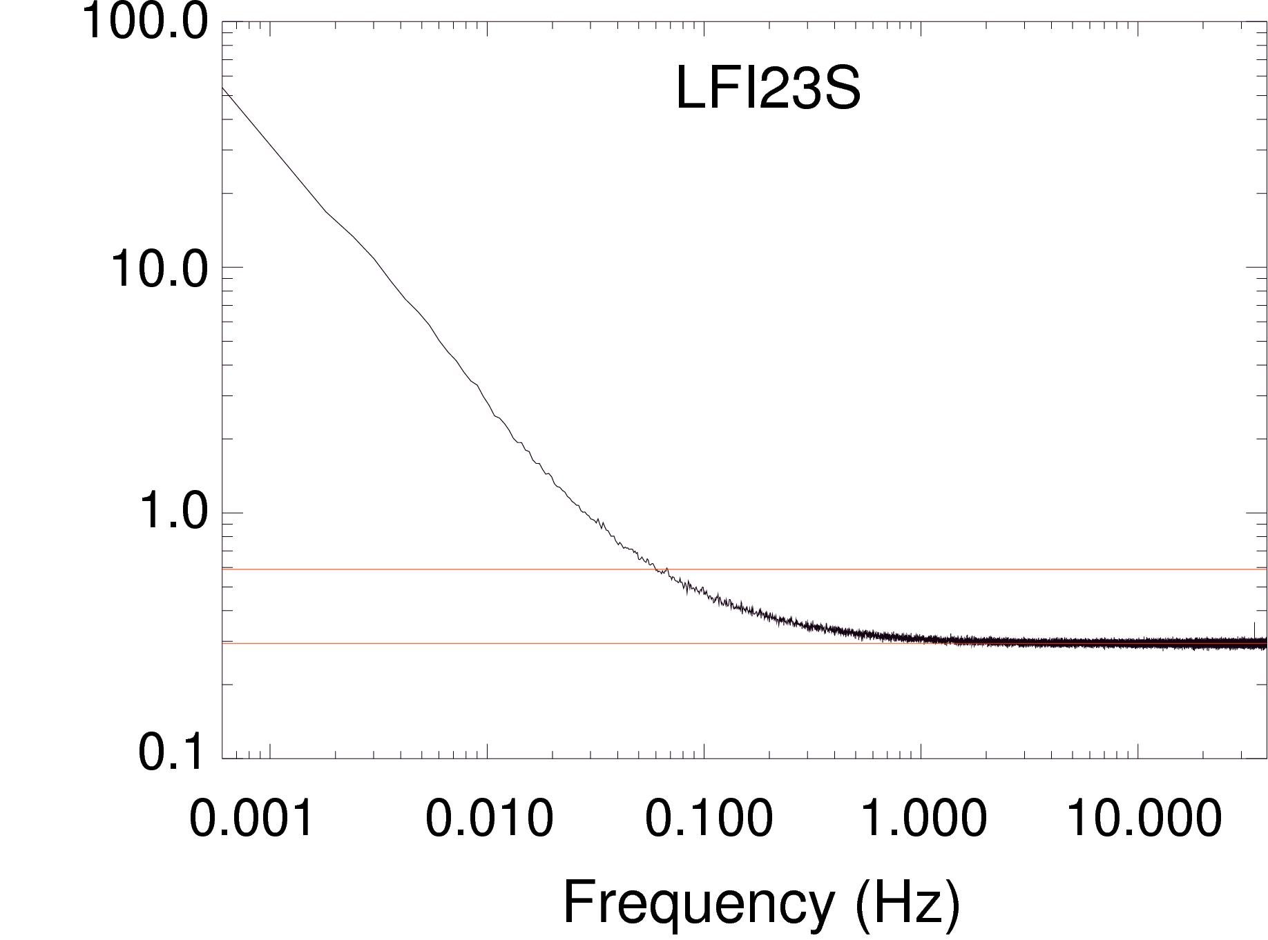
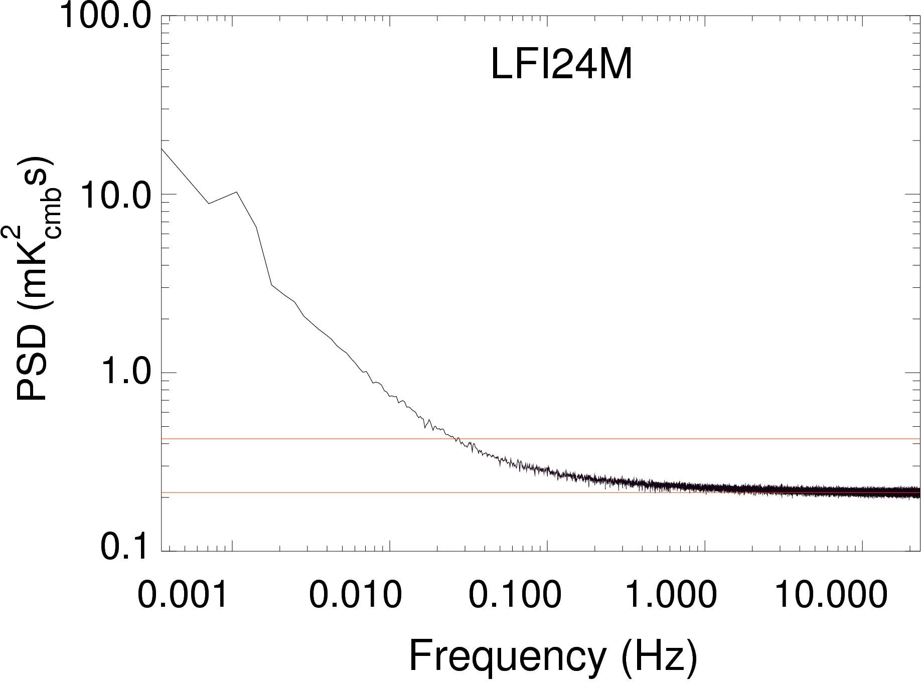
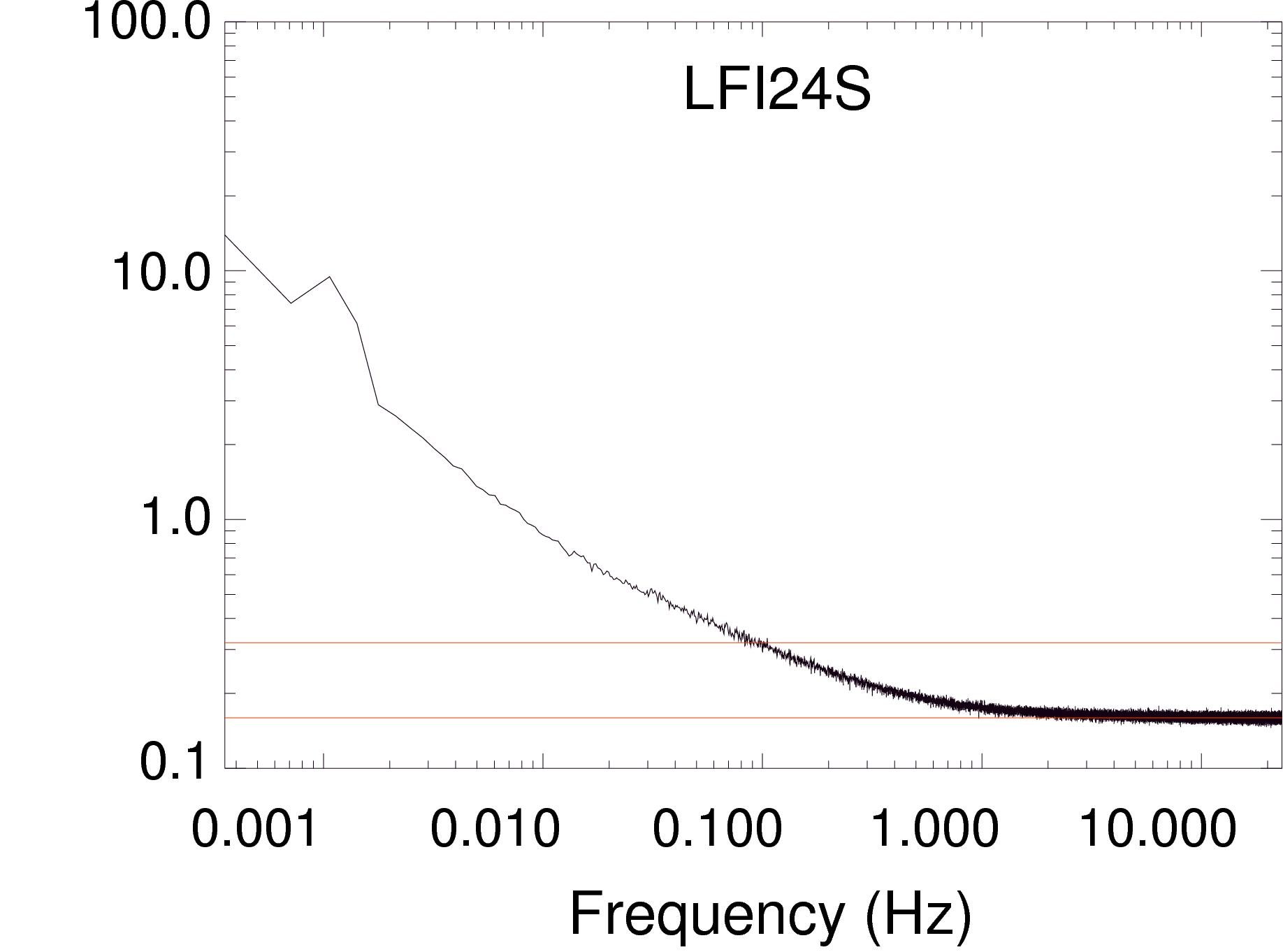
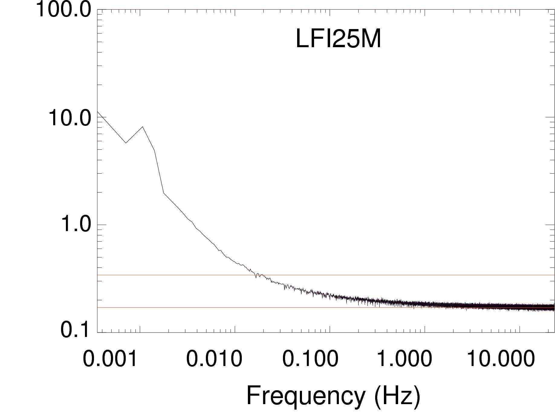
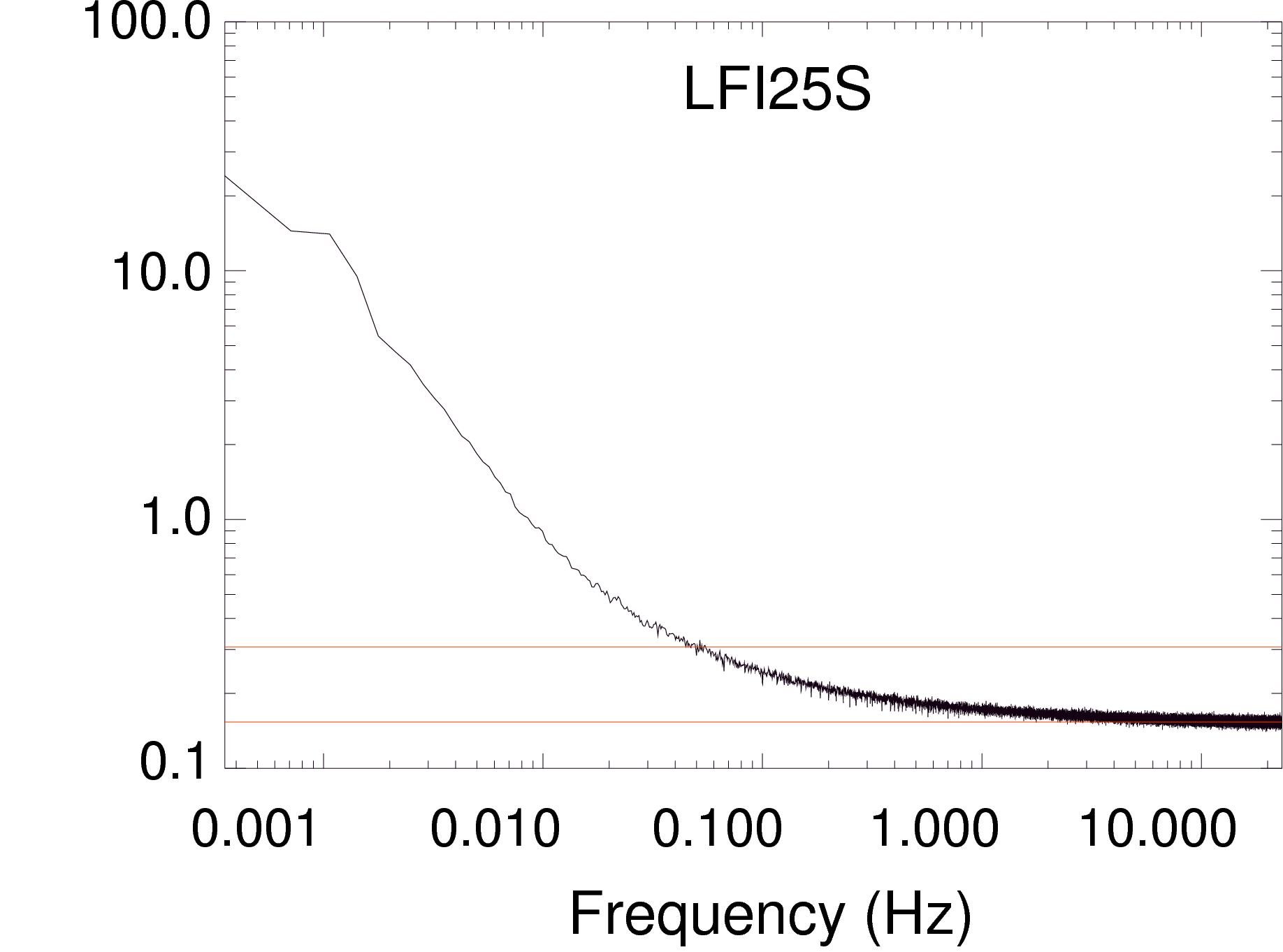
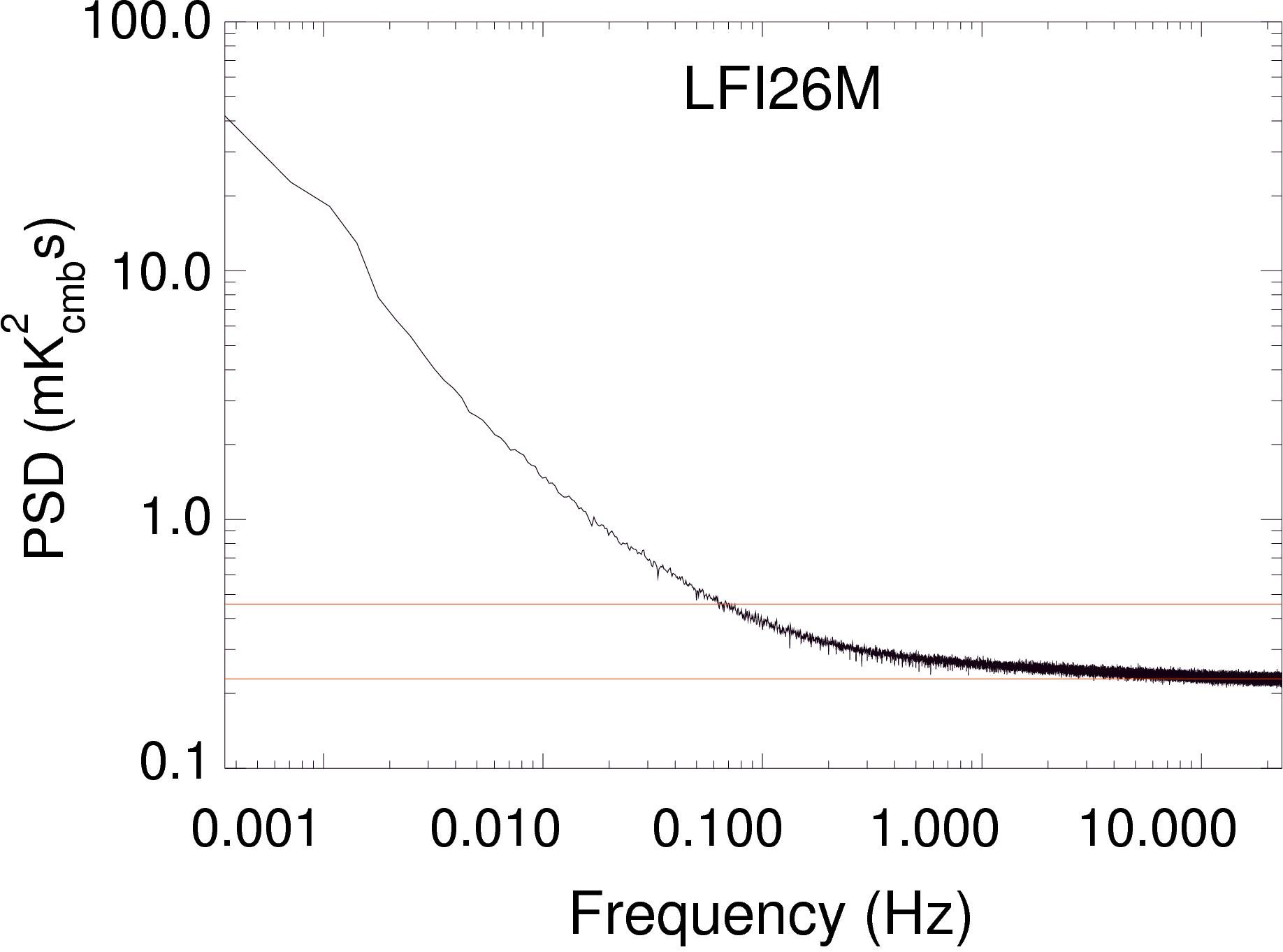
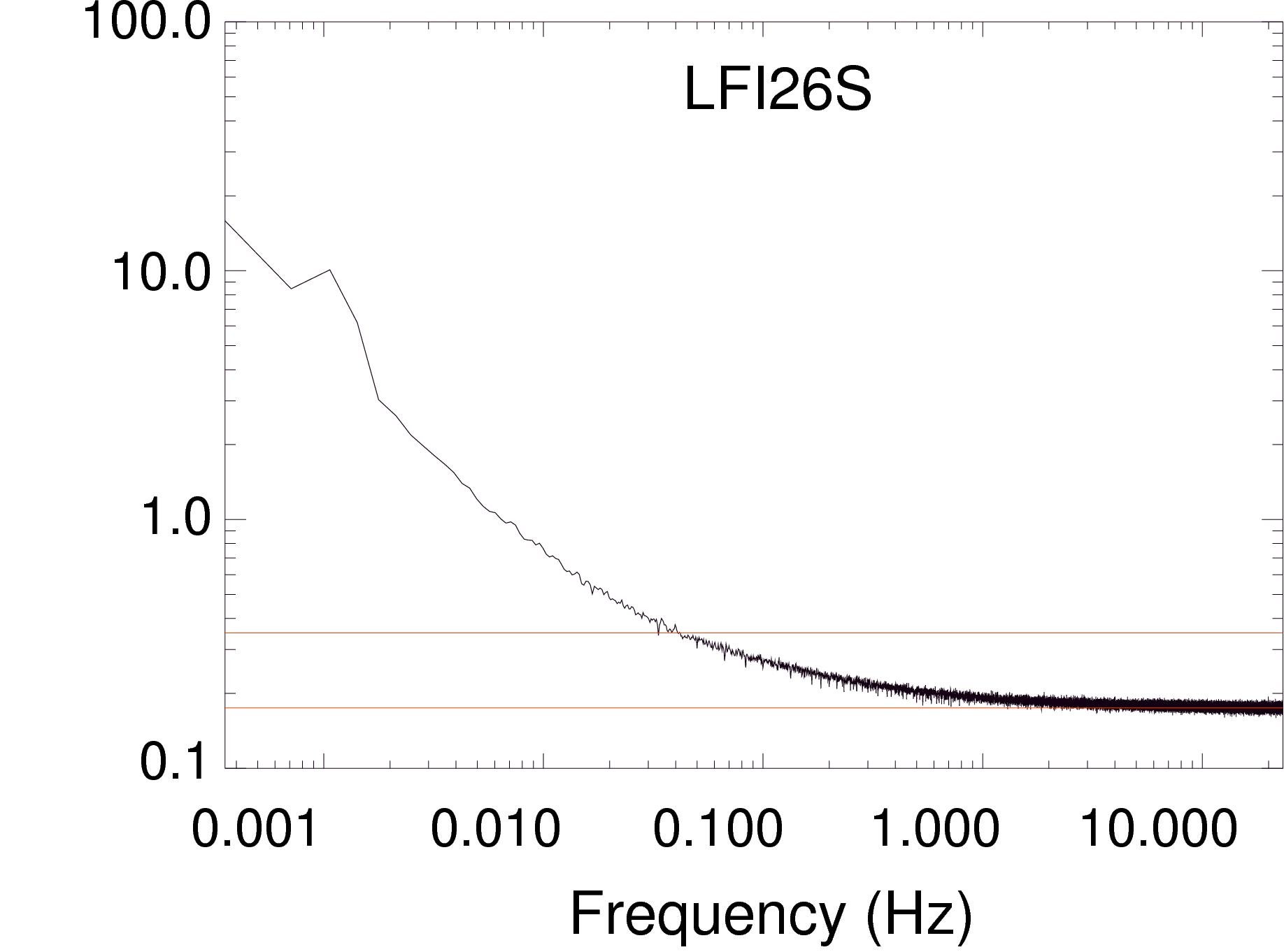
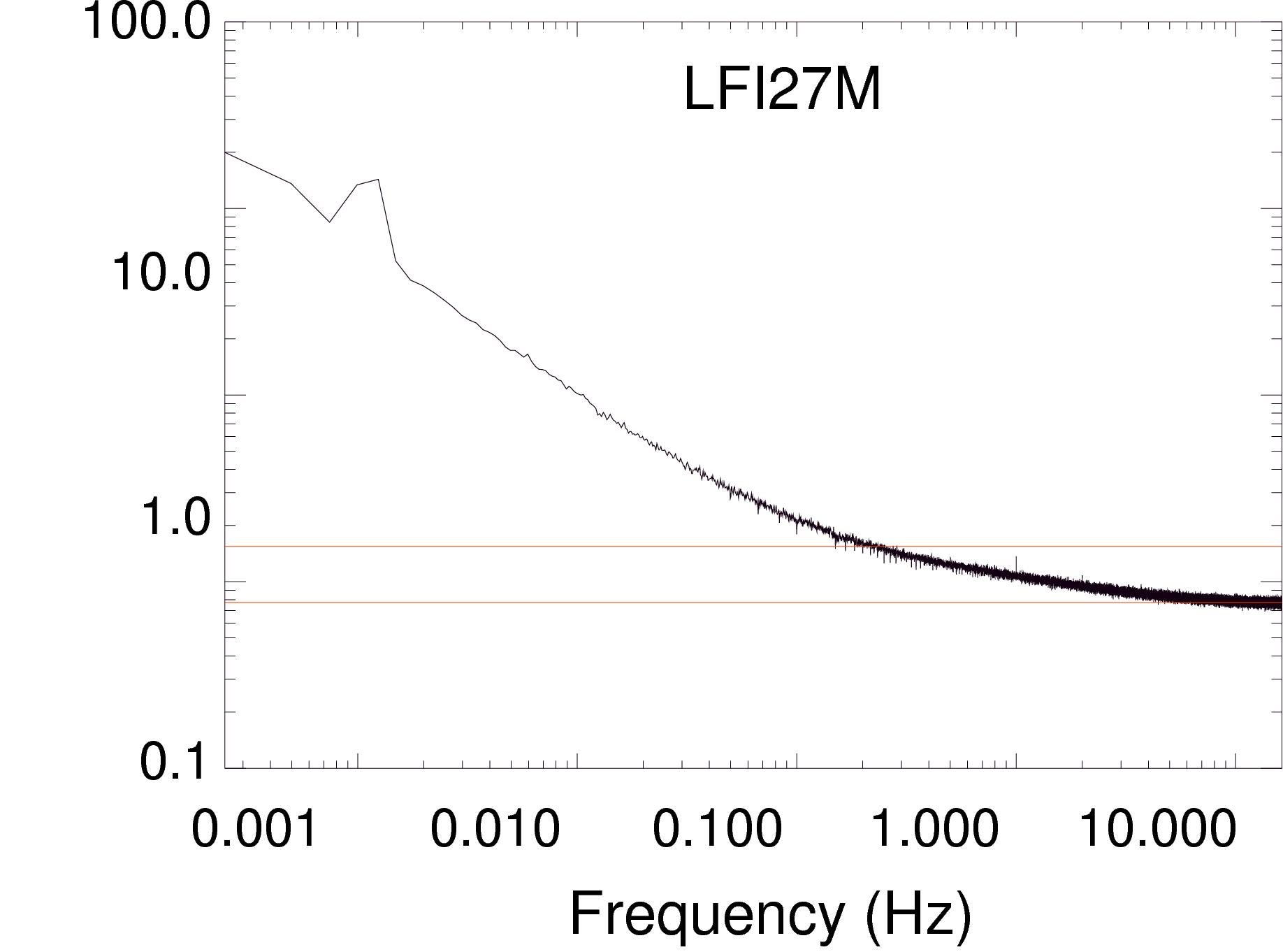
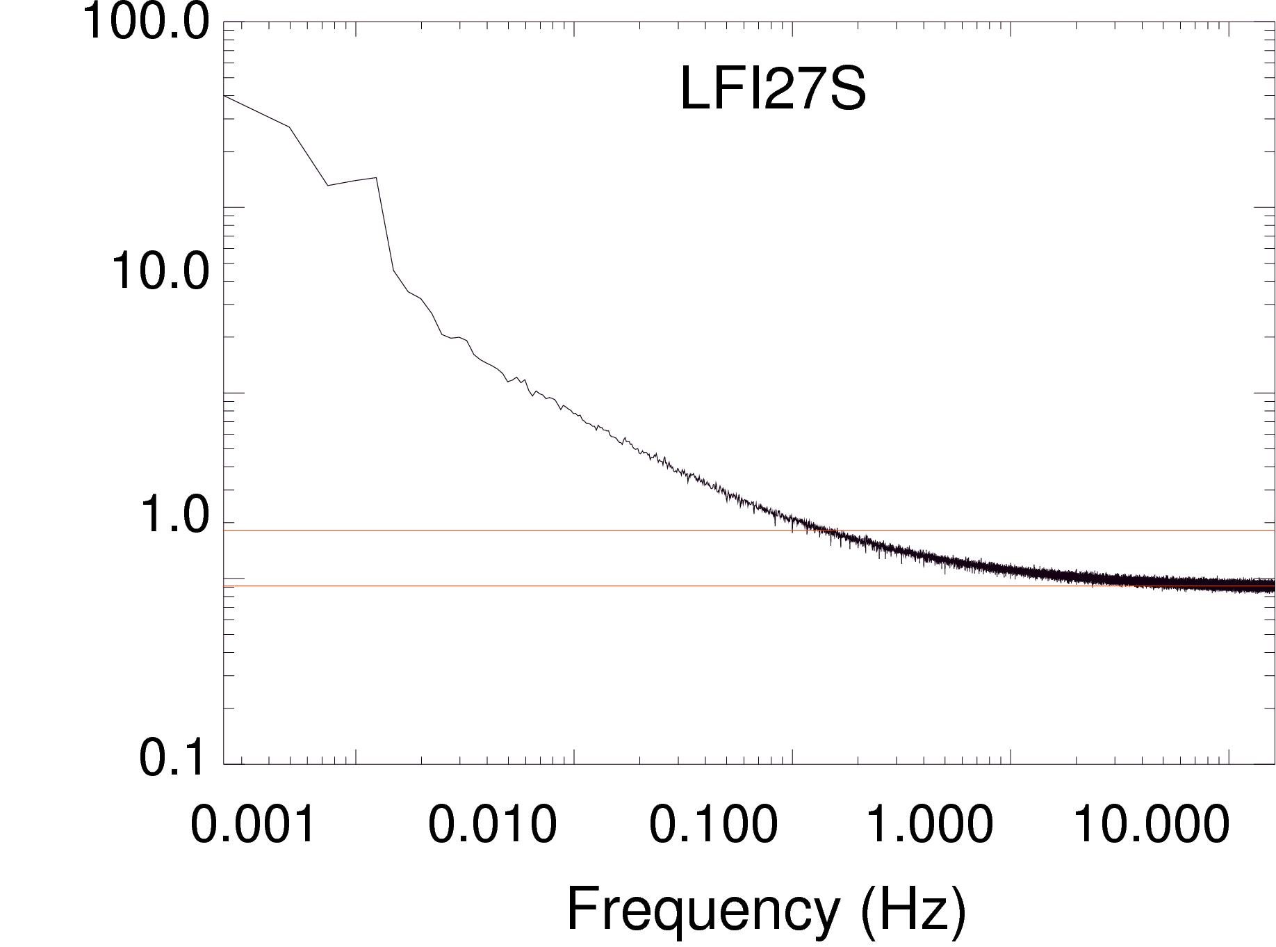
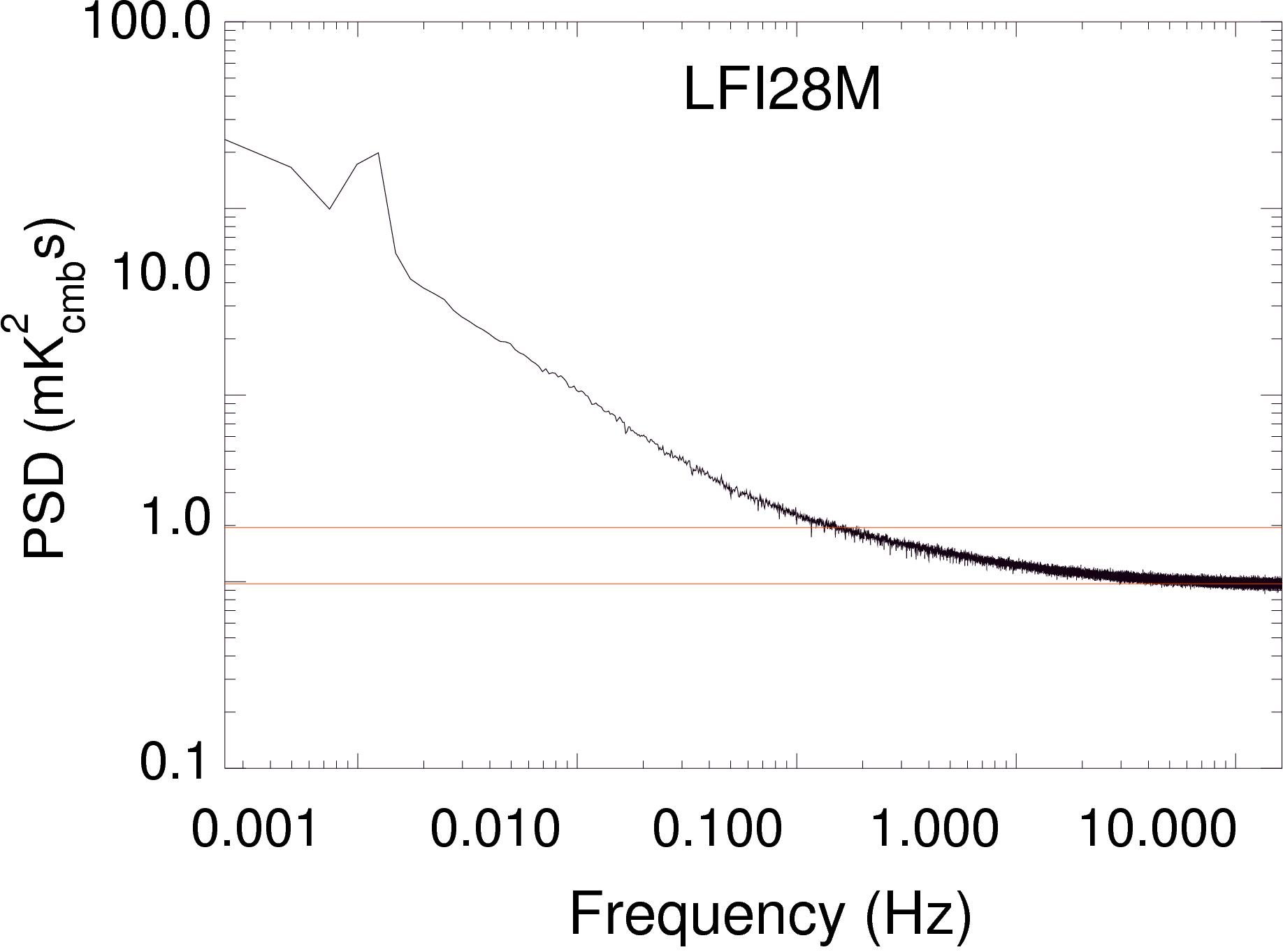
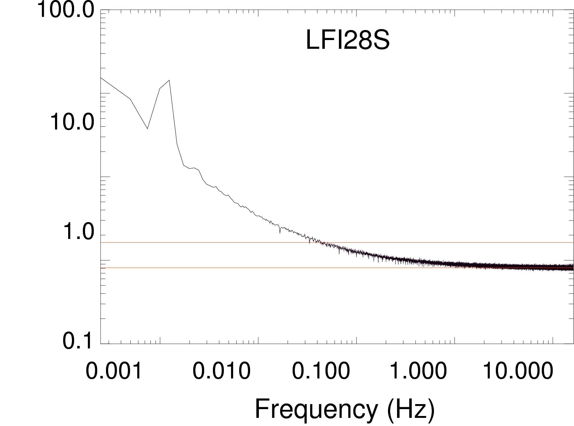
To verify the stability of the instrument, we produced noise estimates from five-day chunks of data separated by 20 days each. Figure 16 gives examples for three radiometers. No significant systematic variations were observed in any of the three parameters, so that final values and uncertainties could be obtained by taking the average and the standard deviation of the five-day values.
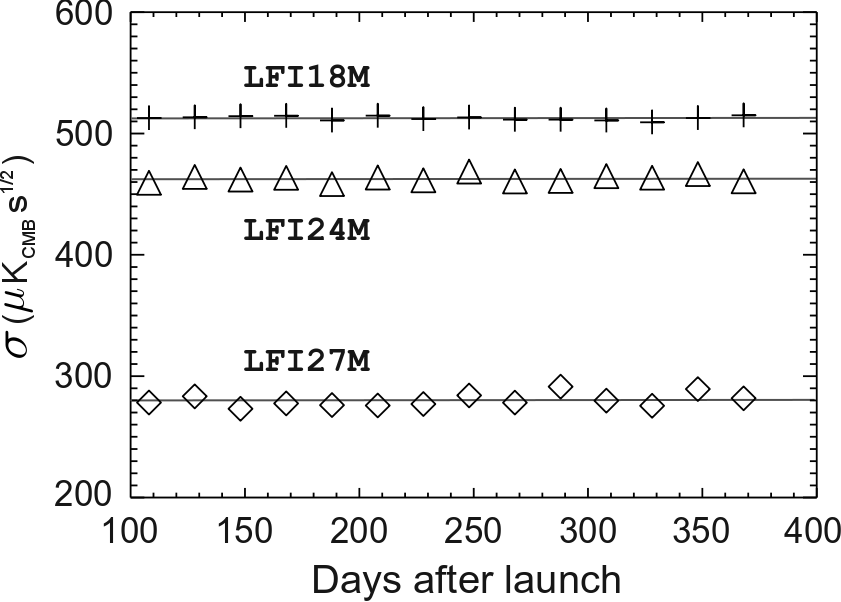
Results for white noise , knee frequency , and slope are reported in Tables 10 and 11. Typical uncertainties are of the order of for the white noise, between 5 and 10% for the slope, and 10 and 20% for the knee frequency. Comparing the noise power spectra for all the 22 LFI radiometers with their best-fit model, we found good agreement as shown in Fig. 17. In the figure, the horizontal red lines represent the white noise level (lower line) and the level of equal contribution from white and noise. The frequency corresponding to the intercept of the upper red line with the power spectrum is the knee frequecy .
|
|||||||||||||||||||||||||||||||||||||||||||||||||||||
|
|||||||||||||||||||||||||||||||||||||||||||||||||||||||||||||||||||||||||||||||||||||||
6.1.2 Jackknife noise maps
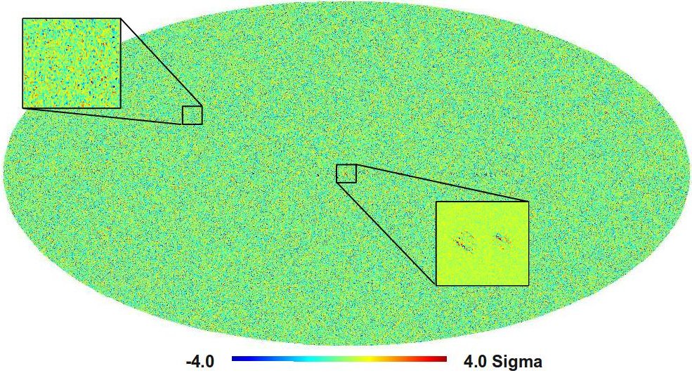
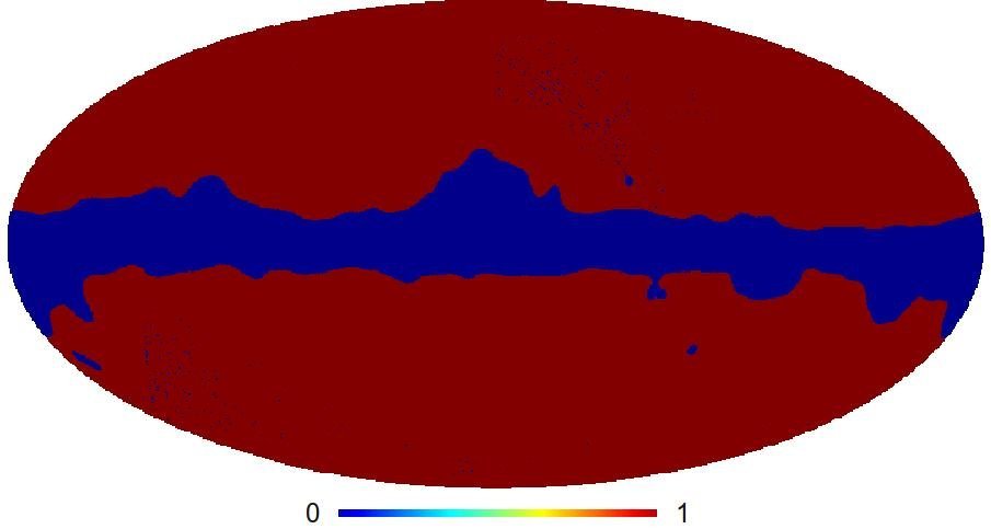
During each pointing period Planck repeatedly scans essentially the same circle in the sky. This provides a powerful method to remove the sky signal and produce maps containing only the instrumental noise (both uncorrelated and correlated on timescales shorter than about 20 minutes). The details of this method are given in Zacchei et al. (2011). These “jackknife” noise maps can be normalised to the white noise estimate at each pixel obtained from the white noise covariance matrix, so that a perfectly white noise map would be Gaussian and isotropic with unit variance. Figure 18 shows an example of such normalised noise maps for the 30 GHz LFI frequency channel. The figure shows a generally structureless map, as expected, apart from a few regions in the Galactic plane where the temperature maps have large gradients over the pixel scale, causing the sky signal to leak into the noise map. In subsequent analysis steps we applied a mask to remove these regions (see Fig. 19). Table 12 gives the standard deviation of normalised noise maps obtained for the three LFI frequencies. Deviations from unity trace the contribution of residual noise in the final maps, which ranges from at 70 GHz to at 30 GHz. A further Gaussianity test performed by calculating skewness and kurtosis of the normalised map after masking the galactic plane yielded null values within two standard deviations of 500 Gaussian simulations.
| 30 GHz | 44 GHz | 70 GHz |
| 1.039 | 1.016 | 1.002 |
6.2 Sensitivity
Fig. 20 compares the calibrated white noise sensitivity for the 22 LFI radiometers calculated from flight data and during ground tests performed both at instrument and satellite level. Error bars reported for values measured in flight and during satellite tests are statistical uncertainties derived from calculations performed on several data chunks888About 20 one-hour chunks for on-ground satellite data, one year of operations for in-flight data.. Error bars reported for values measured at instrument level, instead, represent the uncertainty between two different methods used to extrapolate the white noise sensitivity measured at test conditions ( K input and K front-end temperature) to flight conditions ( K input and K front-end temperature). Further details about this extrapolation are reported in Mennella et al. (2010).
Figure 20 shows general agreement in the sensitivity calculated in various test campaigns, with two outstanding exceptions, radiometers LFI24M and LFI21S, which displayed significantly improved noise levels in-flight. This resulted from an incorrect bias setting of these radiometers during ground tests (see Mennella et al. 2010) and was resolved during in-flight tuning.
In Fig. 20 values for LFI18M and LFI24M measured at instrument-level are not reported because these two radiometers failed. LFI18M was replaced with a spare unit and LFI24M was repaired before instrument delivery (see Mennella et al. 2010).
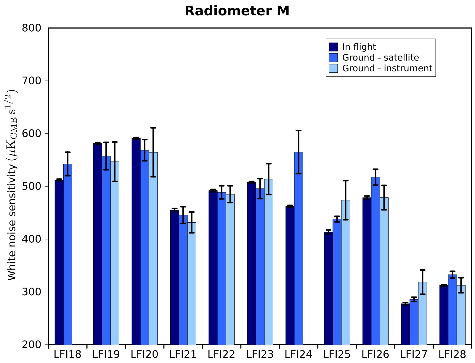
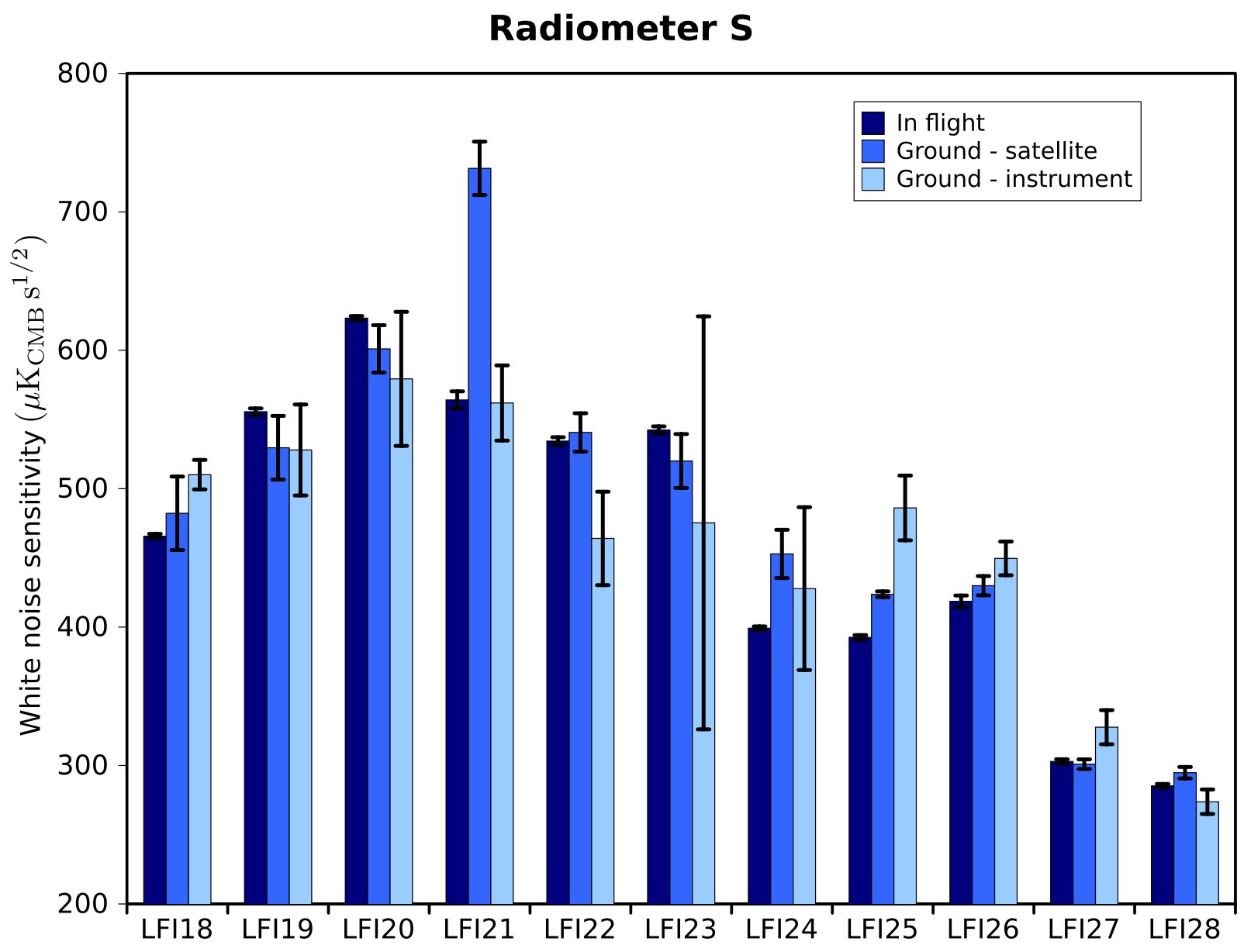
Table 13 summarizes the sensitivity numbers calculated during the first year of operations using methods and procedures outlined in § 6.1 and described in detail in Zacchei et al. (2011) compared with scientific requirements. The measured sensitivity in very good agreement with pre-launch expectations. While the white noise moderately exceeds the design specification, this performance is fully in line with the LFI science objectives.
| Channel | Value | Requir. |
|---|---|---|
| 70 GHz | 152.6 | 119 |
| 44 GHz | 173.1 | 119 |
| 30 GHz | 146.8 | 119 |
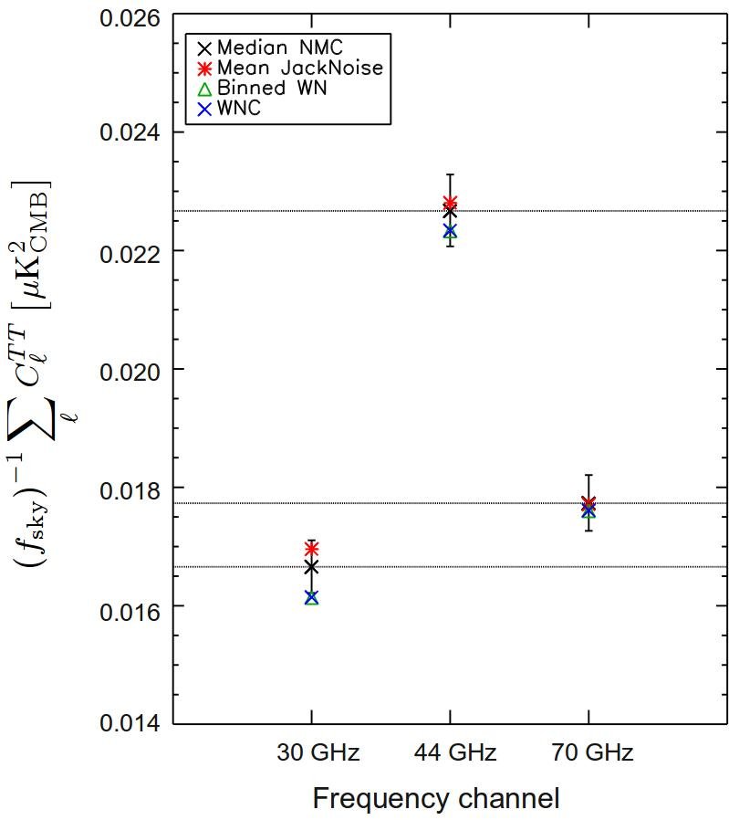
The consistency of the noise estimates outlined in Table 10 was tested by comparing the jackknife noise maps, the white noise covariance matrices, and 101 noise Monte Carlo realisations (see Zacchei et al. 2011, for details). In fact, noise covariance matrices and Monte Carlo simulations are dependent on estimated noise parameters, while the jackknife noise maps describe directly the noise in the final maps.
We produced pseudo- spectra from the jackknife noise maps and noise Monte Carlo maps by anafast (see Fig. 21), and compared high multipole tails () to the predictions from the white noise covariance matrices. In the analysis we masked out a 20% region of the galactic plane and unsolved pixels (pixels that have HEALPix999http://healpix.jpl.nasa.gov bad pixel value in noise maps), leaving us with sky fraction .
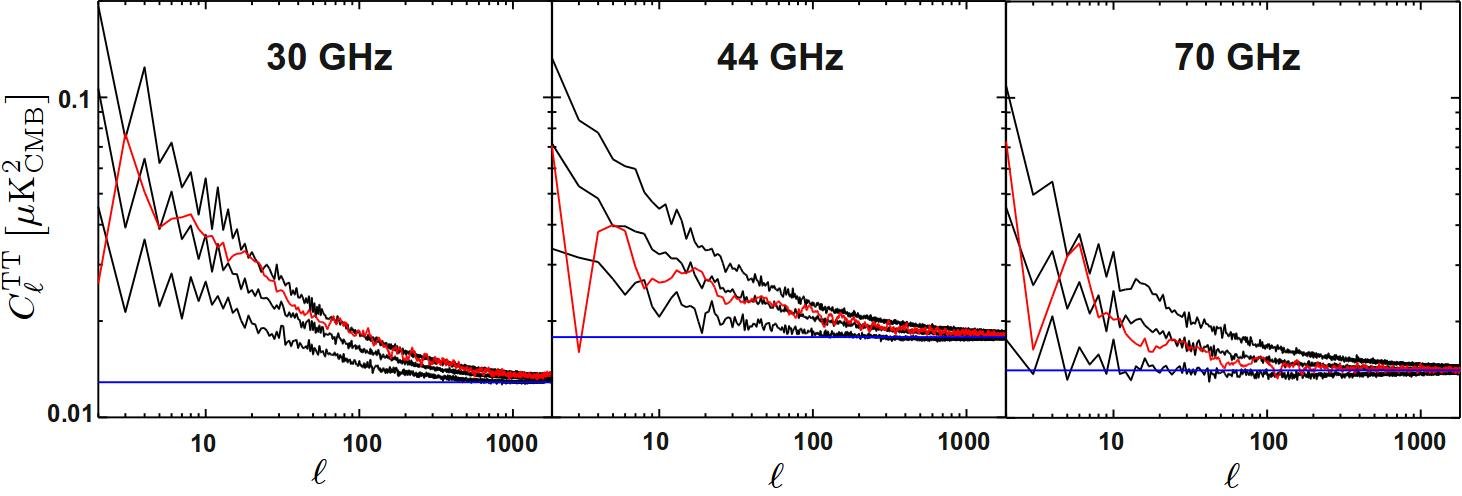
Figure 22 shows a comparison of the noise estimates obtained with the various methods. In the figure the green triangles refer to noise obtained from binned pure white noise Monte Carlo maps, i.e., maps containing no residual noise. At all frequencies the high- mean of the jackknife noise map pseudo- spectra weighted by the inverse sky coverage, (shown in red), are in the 68% range of the noise Monte Carlos (represented with the back error bars). The point from the 30 GHz jackknife noise map is almost 1- higher than the median value for the noise MC due to residual gradient leakage (due to point sources etc.), which is strongest for the 30 GHz channel. The noise power from the white noise covariance matrices and binned maps is always lower than the noise power from the full noise Monte Carlo and jackknife noise maps, as expected, due to residual noise present even at high multipoles. This effect is especially pronounced in the 30 GHz channels, which have larger knee frequencies (see § 6.3).
6.3 Noise properties
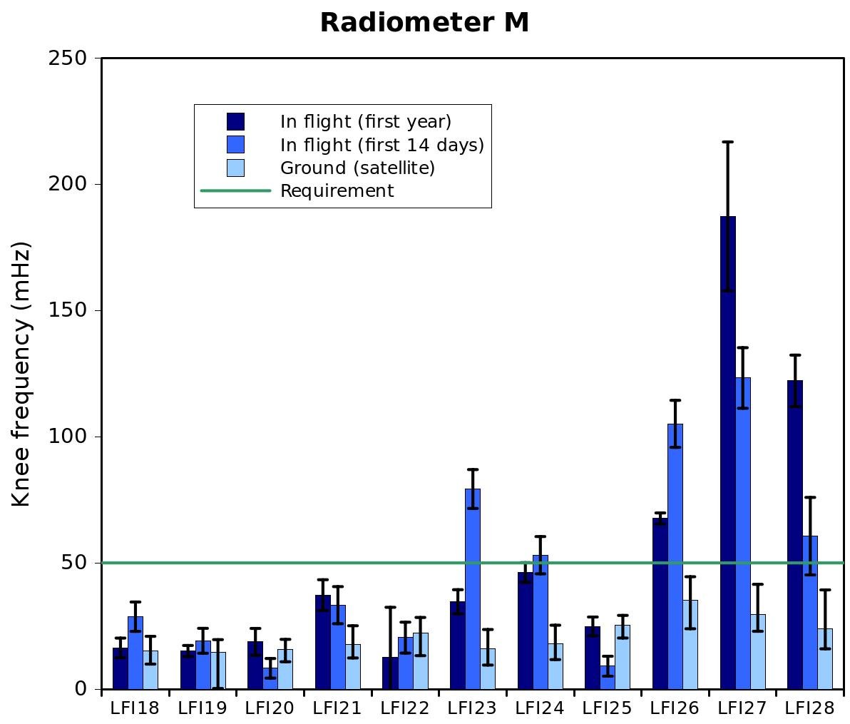
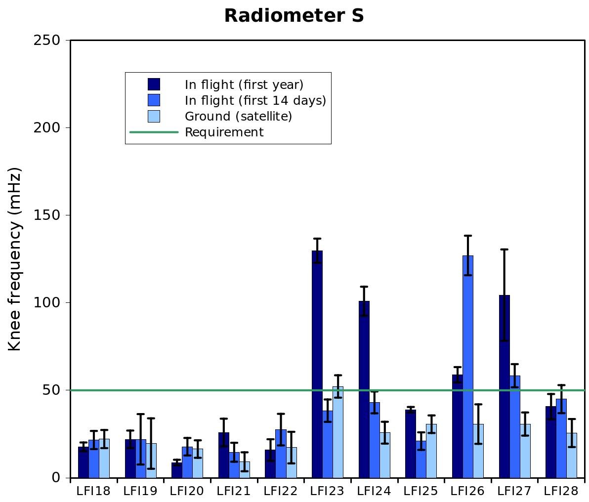
Figure 23 shows a comparison of the knee frequency for the 22 LFI radiometers estimated from flight data and ground satellite calibration. Knee frequency and slope after one year of operations for all LFI radiometers were given earlier in Table 11. With some exceptions the values are below or compatible with requirements and are comparable within the error bars among different measurements.
There are a few cases (LFI23S, LFI24S, LFI27M, LFI28M, LFI27S) in which the knee frequency measured in flight is higher than that measured on ground. The cause is still under investigation, but the impact on the scientific quality of the data is small. Destriping effectively removes correlated structures, limiting the impact of the high knee frequencies to a small () increase of the noise variance (see Table 12 and Fig. 18).
As shown in the low- part of the angular power spectra in Fig. 21, the noise parameters estimated in flight are a good representation of the noise in the actual maps. This means that for cosmological purposes we cannot rely on simple white noise covariance, and a full timeline-to-map Monte Carlo is needed. On the other hand, this also means that there is no need for a more complex functional noise model with respect to the one reported in Eq. (16).
7 First assessment of systematic effects
In this section we discuss the most relevant systematic effects in the first year data. The LFI design was driven by the need to suppress systematic effects well below instrument white noise. The receiver differential scheme, with reference loads cooled to 4 K, greatly minimises the effect of noise and common-mode fluctuations, such as thermal perturbations in the 20 K LFI focal plane. The use of a gain modulation factor (see Eq. (3)) largely compensates for spurious contributions from input offsets. Furthermore, diode averaging (Eq. (6)) allows us to cancel second-order correlations such as those originating from phase switch imbalances.
We have developed an error budget for systematic effects (Bersanelli et al. 2010) as a reference for both instrument design and data analysis. Our goal is to ensure that each systematic effect is rejected to the specified level, either by design or by robust removal in software. At this stage, the following effects proved to be relevant:
-
•
noise (discussed in § 6.3),
-
•
1 Hz frequency spikes,
-
•
thermal fluctuations in the back-end modules driven by temperature oscillations from the transponder during the first survey,
-
•
thermal fluctuations in the 20 K focal plane,
-
•
thermal fluctuations of the 4 K reference loads.
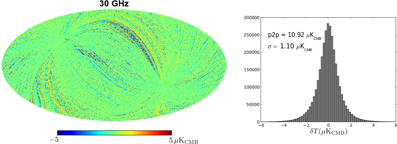
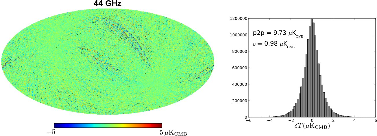
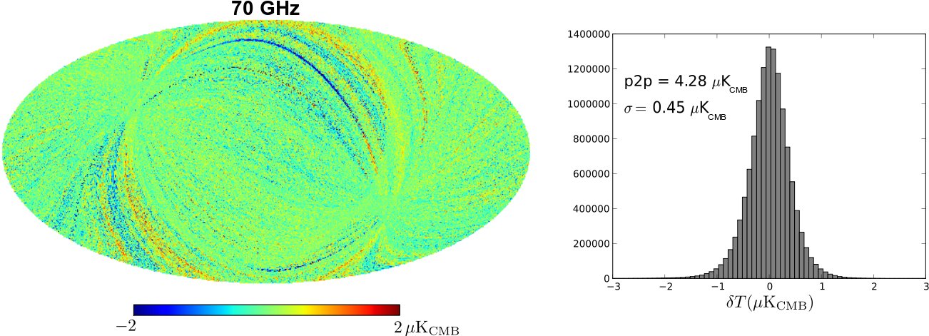
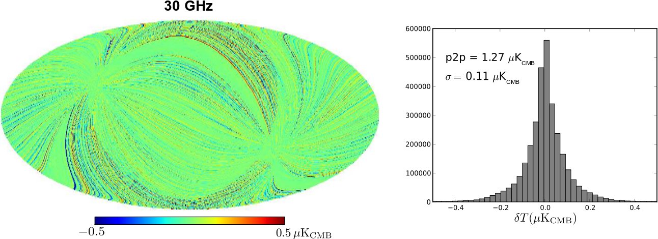
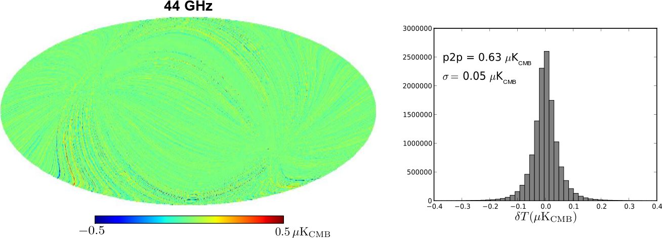
For each of these effects we used flight data and information from ground tests to build timelines, maps, and angular power spectra that represent our best knowledge of their impact on the scientific analysis. Figure 24 shows maps and histograms of the combination of all the above mentioned systematic effects for the three LFI channels. The figure shows that the 30 and 44 GHz channels display a residual level of spurious signals about twice larger than the 70 GHz channel. As shown in the following sections, this is caused by temperature fluctuations of 4 K reference loads that are significantly larger at 30 and 44 GHz than at 70 GHz.
A convenient way to assess the effect on angular power spectra is to calculate the ratio , where is the angular power spectrum of the systematic effect map and is the angular power spectrum of the instrument noise contribution including the residual component remaining after destriping. Figure 25 shows for the three LFI frequency channels. In each panel we have plotted the spectrum obtained from the global maps in Fig. 24 and the spectra derived from the single-component maps (see next sections).
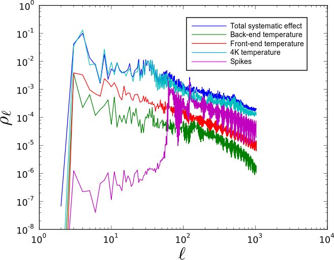
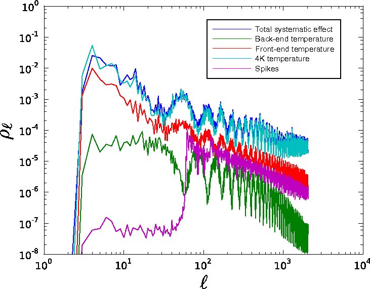
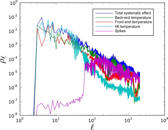
Figure 25 shows that is in the range – for in the range 2–20, and for . The figure also shows that at 30 and 44 GHz the largest contribution to systematic effects is determined by temperature fluctuations of the 4 K reference loads, while the residual systmatic uncertainty in the 70 GHz channel is mainly caused by back-end temperature fluctuations and, at small angular scales, by frequency spikes. Table 14 gives an overview of our current assessment of residual peak-to-peak and rms systematic effects per pixel on LFI temperature maps. Maps were made with at 30 GHz and at 44 and 70 GHz. Corresponding pixel sizes are and .
Further advances in the data analysis pipeline will be aimed at removing spikes from the 70 GHz data, improving relative calibration to account for thermally driven fluctuations, and further suppressing spurious fluctuations caused by 4 K temperature instabilities at 30 and 44 GHz.
| 30 GHz | 44 GHz | 70 GHz | ||||
|---|---|---|---|---|---|---|
| p-p | r.m.s. | p-p | r.m.s. | p-p | r.m.s. | |
| 1-Hz spikes | 4.00 | 0.45 | 1.51 | 0.15 | 2.56 | 0.30 |
| BEM T fluct. | 1.27 | 0.11 | 0.63 | 0.05 | 2.70 | 0.24 |
| FEM T fluct. | 1.05 | 0.23 | 1.15 | 0.22 | 1.12 | 0.21 |
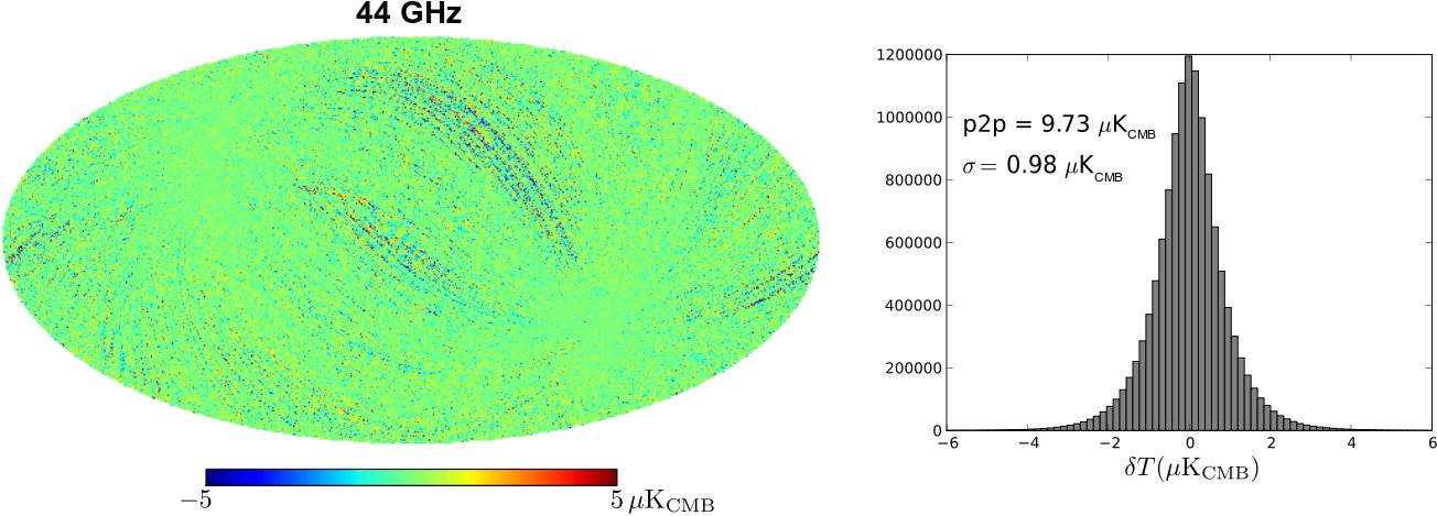
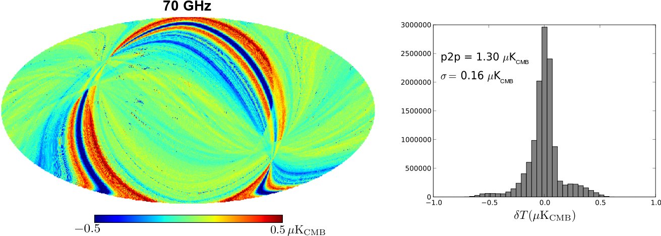
| 4 K T fluct. | 9.76 | 0.98 | 9.73 | 0.98 | 1.30 | 0.16 |
| Totala𝑎aa𝑎aThe total has been estimated from the maps combining all systematic effects (Fig. 24). | 10.92 | 1.10 | 9.73 | 0.98 | 4.28 | 0.45 |
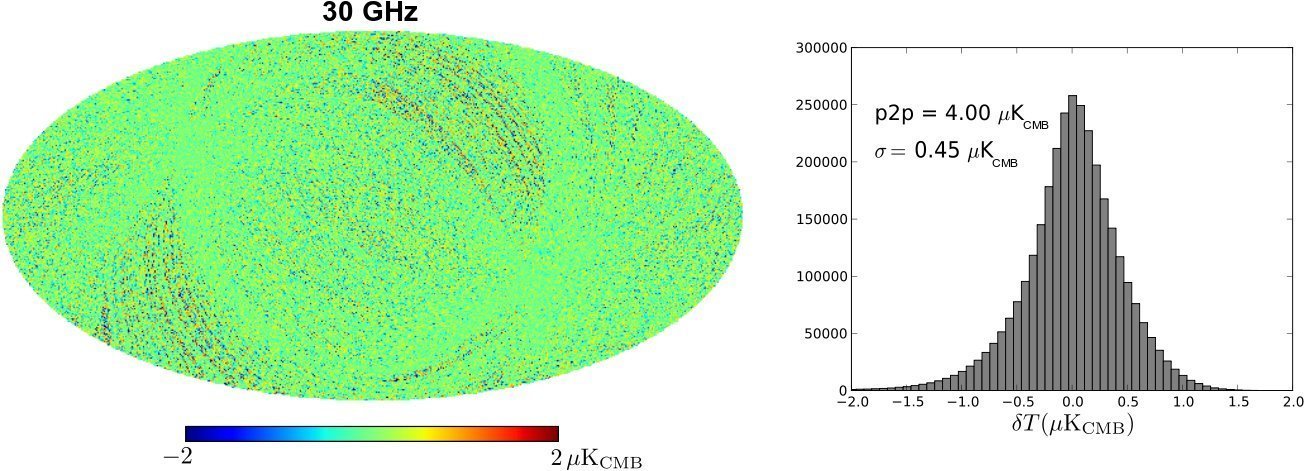
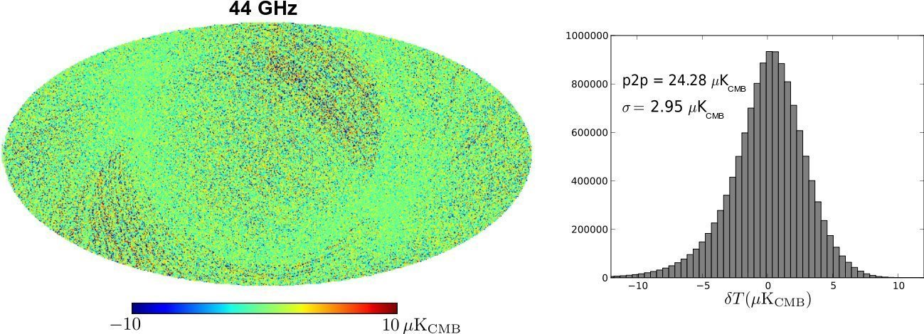
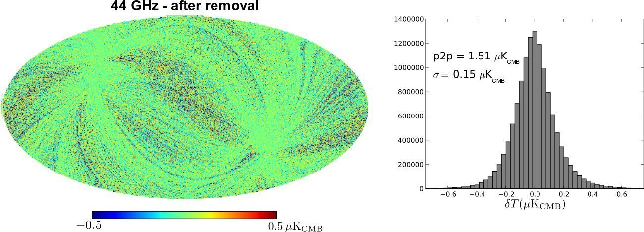
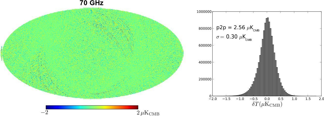
7.1 Frequency spikes
Spikes are seen in the radiometer outputs in the frequency domain at multiples of 1 Hz. These “frequency spikes” were first detected during ground tests, and are caused by pickup from the clock of the housekeeping electronics (Meinhold et al. 2009; Mennella et al. 2010). The pickup occurs between the detector diodes and the DAE gain stage. Frequency spikes are present at some level in the output from all detectors, but affect the 44 GHz data most strongly because of the low voltage output and high DAE gain values in that channel. In this section we provide estimates of the residual systematic effect after frequency spike removal at 44 GHz, and the effect caused by the spikes without any removal at 30 and 70 GHz.
In the time domain, the frequency domain spikes comprise a one second square wave with a rising edge near 0.5 s and a falling edge near 0.75 s in on-board time. During the first year of operations we did not observe any deviation in either the phase or the shape of these signals.
Templates of these spurious square waves obtained from the output voltages have been used to remove this effect from the data before differentiation (procedures and algorithms are described in Zacchei et al. (2011)). Although we could in principle apply the removal process to all data, we decided to remove the spikes only from the 44 GHz data, which are the most affected by this effect.
To estimate the residual in the spike removal process caused by slow variations in the square wave amplitude, we used a simple minimisation procedure to estimate the amplitude of the template for each hour of data, then smoothed the amplitude by simple binning with a 10-day window size. We took this smoothed amplitude as our estimate of the true time variation of the spike signal, and calculated the residual error that would result if we approximated this time-varying signal with a constant template in the spike removal process. Although we could use, in principle, the time-varying template to remove the effect, we decided to use the simplest and most robust approach of a constant-amplitude template. The possibility to implement of a model that accounts for slow spike amplitude drifts will be considered for future data releases.
Templates were also used to generate maps for each frequency channel to determine the impact of the spike signal on the science results. These maps and the corresponding histograms are shown in Fig. 26. For the 44 GHz channel we also show the residual effect after removing the constant template, showing that after removal the residual effect is reduced by a factor of about 20.
7.2 Thermal fluctuations
The LFI is sensitive to temperature fluctuations of the warm back-end unit, the 20 K focal plane, and the 4 K reference loads. In the first two, temperature variations impact the sky and reference load signals at a similar level, so that in the differential radiometric output the residual spurious variations are reduced by more than one order of magnitude. Fluctuations at the level of the 4 K reference loads, instead, transfer directly to the radiometric output, and may represent a more critical source of systematic errors.
The effects of low frequency thermal fluctuations are strongly suppressed by the spacecraft spin itself and the destriping map-making codes (Zacchei et al. 2011). High frequency thermal fluctuations are strongly damped by the thermo-mechanical structure of the spacecraft and instruments (Tomasi et al. 2009). The dominant effects, then, come from fluctuations at frequencies in a range around the spin frequency.
In this section we present an overview of the impact on the LFI science caused by the residual level of systematic effects in the final maps using a dedicated pipeline that follows the procedure outlined below.
-
•
Start from a time ordered datastream of a temperature sensor representative of the temperature behaviour of the considered thermal stage;
-
•
low-pass filter to remove high-frequency sensor noise;
-
•
apply thermal transfer functions where appropriate to obtain the physical temperature behaviour at the level of the receiver components sensitive to the fluctuation;
-
•
apply the radiometric transfer function to convert the physical temperature fluctuation into antenna temperature fluctuation;
-
•
resample at scientific sampling frequency, calibrate and build differenced time-ordered data;
-
•
build maps with Madam.
These maps have been generated combining actual flight housekeeping data with thermal and radiometric transfer functions obtained from flight and ground-test data (Terenzi et al. 2009). They represent, therefore, our current best estimate of the impact of the individual effects on the science in flight conditions.
As explained in § 5.3 further developments of this work will aim at including thermal fluctuations from the back-end unit in the calibration model which will reduce the need to remove the spurious signal from the time ordered data during map-making.
7.2.1 Back-end temperature fluctuations
As mentioned in § 5.1, for the first 258 days of the mission the satellite transponder was switched on only for the daily telecommunication period. This induced quasi-sinusoidal fluctuations in the Planck service module temperature that propagated to the LFI back-end unit, and were recorded by the instrument housekeeping sensors at the level of K/day.
This temperature variation drives variation in the total power voltage output of both sky and reference detectors, which largely disappears in the difference, shown in Fig. 12. The effect on the undifferenced total power data, however, was useful in calculating correlation coefficients between temperature and voltage outputs. These coefficients have been used to estimate the residual effect on time-ordered data and maps. Figure 27 shows this correlation for the detector LFI27M-00.
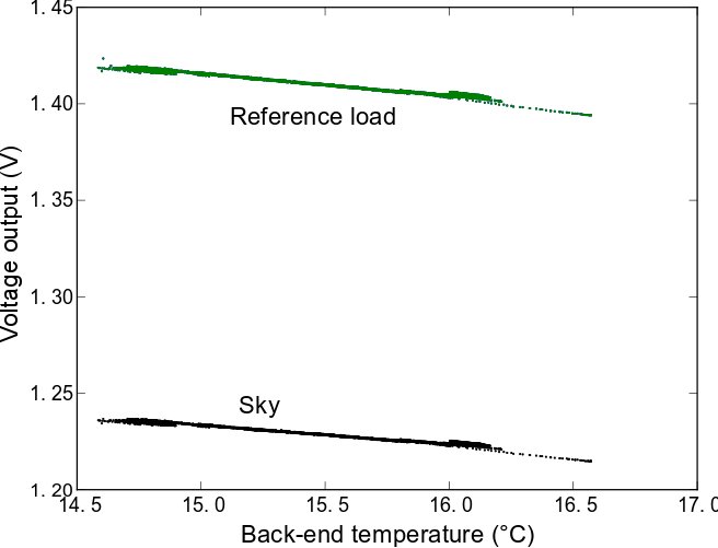
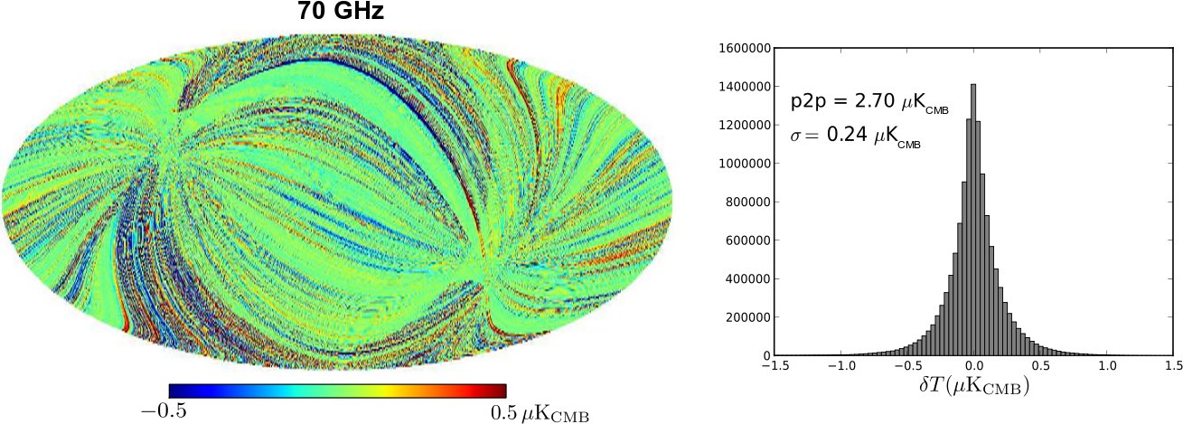
Figure 28 shows the expected systematic effects of temperature fluctuations of the back-end unit during the first year of operations. The peak-to-peak effect is , and the rms is well below .
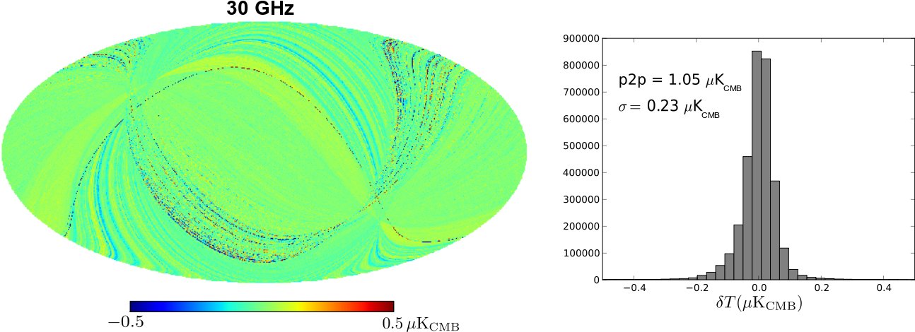
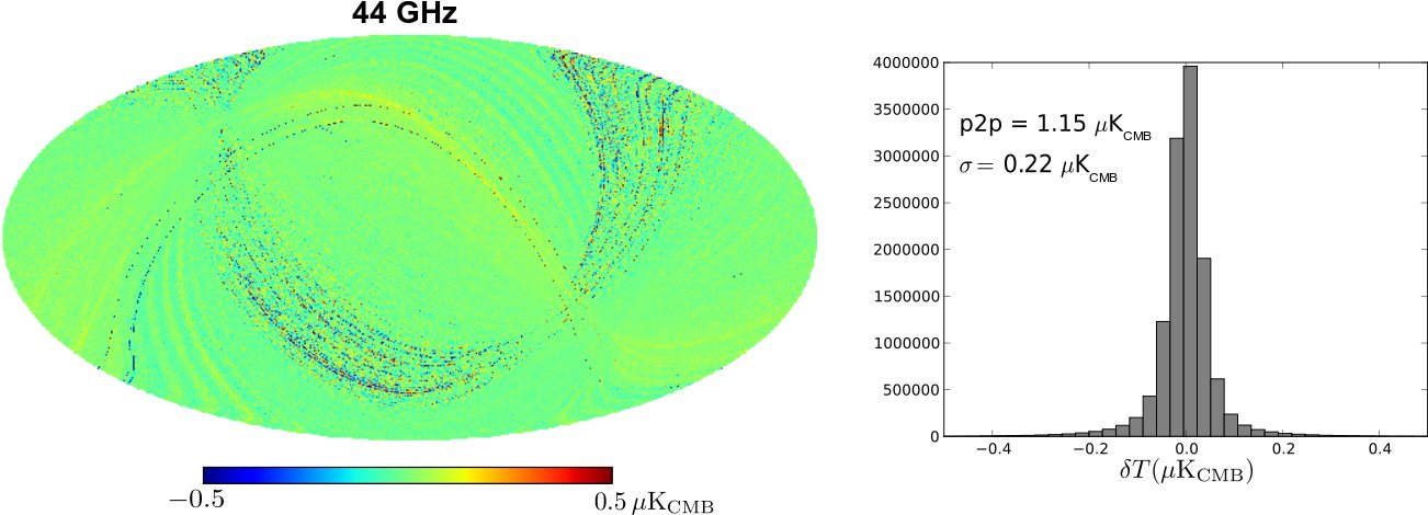
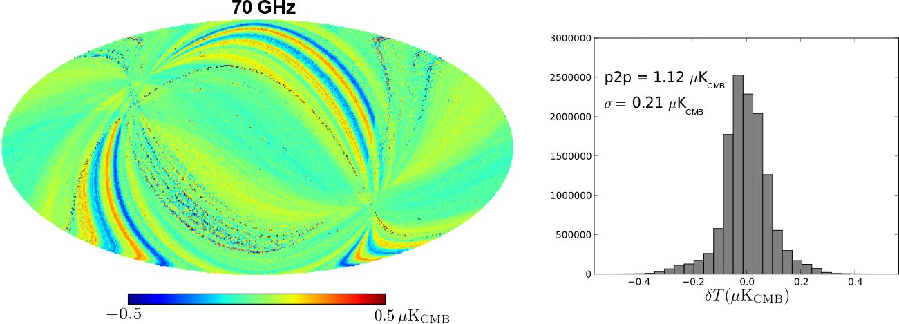
7.2.2 Front-end temperature fluctuations
Another source of temperature fluctuations is the Planck sorption cooler (Morgante et al. 2009; Planck Collaboration 2011b), which displays temperature variations of the order of K peak-to-peak at the cold end attached to the LFI focal plane unit. These fluctuations are damped by a thermal stabilisation assembly (TSA; Planck Collaboration 2011b) down to about 100 mK peak-to-peak at low frequency.
During the second half of the first year of operations the expected cooler degradation led to an increase of the cold end temperature and the low-frequency fluctuations. At the radiometers the temperature increased by about 0.2 K, with fluctuations running about 30 mK peak-to-peak. We estimated the effect of these fluctuations on the science data using ground-measured transfer functions that include the effect of temperature on both gain and noise. Figure 29 shows the calculated effects for the three LFI frequency channels. As in the case of back-end temperature fluctuations, the overall effect is peak-to-peak and rms.
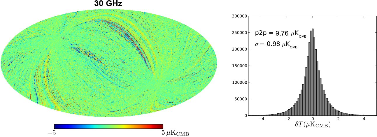
7.2.3 4 K reference load temperature fluctuations
The temperature stability of the 4 K reference loads, attached to the HFI 4 K mechanical box, is a key factor in the LFI systematic effects budget. Temperature fluctuations of the loads are driven primarily by fluctuations at the 20 K cold-end interface, which propagate to the LFI reference loads by conduction through the HFI mounting struts and radiation from the LFI. See Planck Collaboration (2011b) for details.
The 70 GHz reference loads are mounted close to the HFI 4 K plate and are stabilised by proportional-integral-derivative (PID) active controllers that remove almost completely low frequency fluctuations. The loads at 30 and 44 GHz are farther from the HFI 4 K plate and closer to the HFI mounting struts; their temperature is less stable. Details of temperature sensor measurements are provided in Planck Collaboration (2011b).
This difference is reflected in the maps shown in Fig. 30, where the residual systematic effect in the 30 and 44 GHz channels is times larger than in the 70 GHz channel. Nevertheless, given the reduction provided by destriping, the residual systematic is several times below the instrument noise, as shown by the angular power spectra in Fig. 25. Further work will be aimed at correlating radiometric and housekeeping data to further reduce the residual effect caused by these fluctuations.
8 Summary of main performance parameters
Table 15 gives a top-level summary of instrument performance parameters measured in flight. Optical properties have been successfully reconstructed using Jupiter transits and the main parameters are in agreement with pre-launch estimates. Also the white noise sensitivity agrees with ground measurements; for some channels sensitivity improved after in-flight bias tuning. Parameters describing the noise component are in line with ground measurements and the 50 mHz requirement except at 30 GHz. That channel that has a knee frequency over 100 mHz, which is, however, well-handled by destriping. Absolute photometric calibration based on the CMB dipole yields an overall statistical uncertainty of . Variations due to slow instrumental variations are traced by the calibration pipeline, yielding an overall uncertainty ranging between 0.05% and 1%. The residual systematic uncertainty is of the order of 1 K rms per pixel. Average colour corrections are provided in Table 2.
|
9 Conclusions
We have discussed the scientific performance of the Planck Low Frequency Instrument after one year of operations.
Since the start of Planck nominal operations, the LFI has shown excellent stability in all measured parameters. The instrument uninterruptedly observed the microwave sky with negligible data loss and less than 1% discarded data because of anomalies. Typical variations in the instrumental output were less than 1% on time scales of several days and were mainly driven by slow thermal fluctuations.
The main beams have been reconstructed down to dB using Jupiter as a source, with results closely matching those expected from simulations. In-flight measurements of white noise sensitivity are in very good agreement with ground results, with significant improvements in some channels thanks to in-flight bias tuning. The impact of low frequency noise is very small, especially at 70 GHz where the measured knee frequency is about 30 mHz, almost twice better than the requirement. At 30 GHz the noise is higher than measured on the ground, with a knee frequency of about 100 mHz. Residual fluctuations in the timestreams, however, are effectively removed during map-making, as expected from several pre-launch simulation studies (Kurki-Suonio et al. 2009; Poutanen et al. 2004; Keihänen et al. 2004). We have shown that the noise increase due to the component is a few percent at 30 and 44 GHz, and only 0.2% at 70 GHz.
Photometric calibration is based on the CMB dipole via an iterative procedure explained in Zacchei et al. (2011). Excellent absolute calibration accuracy of will likely be improved still further in future analyses by using the orbital dipole as absolute calibrator. Our current relative calibration traces gain variations on timescales larger than 5–10 days, yielding an overall statistical accuracy in the range 0.05–0.1%. Thermally-driven gain fluctuations on smaller timescales are currently not implemented in our gain model and contribute as a systematic uncertainty in the final maps. A new version of the gain model, now being developed, will take into account the effect of such fluctuations to further reduce this residual uncertainty.
We have presented a preliminary analysis of all the systematic effects that are relevant at this stage of the analysis. Their impact on LFI science has been evaluated by projecting each effect on full-sky maps and angular power spectra through a dedicated pipeline that exploits radiometric and housekeeping data in conjuction with external parameters measured in ground or flight tests, such as thermal susceptibilities or spike characteristics. The combined residual effect from frequency spikes and thermal instabilities (in the 4 K, 20 K, and 300 K stages) is several order of magnitudes below the instrumental noise at all angular scales smaller than 10∘, and less than 10% at larger scales.
The overall performance of LFI as measured in-flight demonstrates an instrument with unprecedented combination of sensitivity, angular resolution and suppression of systematic errors for full-sky imaging at these frequencies. In particular, the control of systematic effects and non-white noise components represent key challenges for accurate extraction of the cosmological information encoded in the temperature and polarisation maps. Our preliminary assessment shows that, even without dedicated de-correlation of thermal effects, the LFI is already largely immune to instrumental effects, with prospects of further suppression after implementing a more representative gain model and temperature fluctuation removal algorithms.
One more year of continuous observations is currently planned for Planck, with a further LFI extension to the maximum lifetime allowed by the sorption cooler. Everything to date suggests that the instrument will maintain its performance throughout the remaining period and provide rich and high-quality scientific data that will be explored for many years to come.
Acknowledgements.
Planck is too large a project to allow full acknowledgement of all contributions by individuals, institutions, industries, and funding agencies. The main entities involved in the mission operations are as follows. The European Space Agency operates the satellite via its Mission Operations Centre located at ESOC (Darmstadt, Germany) and coordinates scientific operations via the Planck Science Office located at ESAC (Madrid, Spain). Two Consortia, comprising around 50 scientific institutes within Europe, the USA, and Canada, and funded by agencies from the participating countries, developed the scientific instruments LFI and HFI, and continue to operate them via Instrument Operations Teams located in Trieste (Italy) and Orsay (France). The Consortia are also responsible for scientific processing of the acquired data. The Consortia are led by the Principal Investigators: J.-L. Puget in France for HFI (funded principally by CNES and CNRS/INSU-IN2P3) and N. Mandolesi in Italy for LFI (funded principally via ASI). NASA’s US Planck Project, based at JPL and involving scientists at many US institutions, contributes significantly to the efforts of these two Consortia. In Finland, the Planck LFI 70 GHz work was supported by the Finnish Funding Agency for Technology and Innovation (Tekes). This work was also supported by the Academy of Finland, CSC, and DEISA (EU). Some of the results in this paper have been derived using the HEALPix package (Górski et al. 2005). A description of the Planck Collaboration and a list of its members can be found at http://www.rssd.esa.int/index.php?project=PLANCK&page=Planck_Collaboration.References
- Bersanelli et al. (2010) Bersanelli, M., Mandolesi, N., Butler, R. C., et al. 2010, A&A, 520, A4+
- Cuttaia et al. (2009) Cuttaia, F., Mennella, A., Stringhetti, L., et al. 2009, Journal of Instrumentation, 4, 2013
- D’Arcangelo et al. (2009) D’Arcangelo, O., Figini, L., Simonetto, A., et al. 2009, Journal of Instrumentation, 4, 2007
- Davis et al. (2009) Davis, R. J., Wilkinson, A., Davies, R. D., et al. 2009, Journal of Instrumentation, 4, 2002
- de Gasperis et al. (2005) de Gasperis, G., Balbi, A., Cabella, P., Natoli, P., & Vittorio, N. 2005, A&A, 436, 1159
- Górski et al. (2005) Górski, K. M., Hivon, E., Banday, A. J., et al. 2005, ApJ, 622, 759
- Gregorio et al. (2011) Gregorio, A., Mennella, A., Cuttaia, F., et al. 2011, The in-flight calibration and verification of the Planck-LFI instrument (To be submitted to Journal of Instrumentation)
- Herreros et al. (2009) Herreros, J. M., Gómez, M. F., Rebolo, R., et al. 2009, Journal of Instrumentation, 4, 2008
- Hinshaw et al. (2009) Hinshaw, G., Weiland, J. L., Hill, R. S., et al. 2009, ApJS, 180, 225
- Jarosik et al. (2011) Jarosik, N., Bennett, C. L., Dunkley, J., et al. 2011, ApJS, 192, 14
- Keihänen et al. (2010) Keihänen, E., Keskitalo, R., Kurki-Suonio, H., Poutanen, T., & Sirviö, A. 2010, A&A, 510, A57+
- Keihänen et al. (2005) Keihänen, E., Kurki-Suonio, H., & Poutanen, T. 2005, MNRAS, 360, 390
- Keihänen et al. (2004) Keihänen, E., Kurki-Suonio, H., Poutanen, T., Maino, D., & Burigana, C. 2004, A&A, 428, 287
- Kogut et al. (1996) Kogut, A., Banday, A. J., Bennett, C. L., et al. 1996, ApJ, 470, 653
- Kurki-Suonio et al. (2009) Kurki-Suonio, H., Keihänen, E., Keskitalo, R., et al. 2009, A&A, 506, 1511
- Lamarre et al. (2010) Lamarre, J., Puget, J., Ade, P. A. R., et al. 2010, A&A, 520, A9+
- Ludwig (1973) Ludwig, A. 1973, IEEE Transactions on Antennas and Propagation, 21, 116
- Mandolesi et al. (2010) Mandolesi, N., Bersanelli, M., Butler, R. C., et al. 2010, A&A, 520, A3+
- Maris et al. (2009) Maris, M., Tomasi, M., Galeotta, S., et al. 2009, Journal of Instrumentation, 4, 2018
- Meinhold et al. (2009) Meinhold, P., Leonardi, R., Aja, B., et al. 2009, Journal of Instrumentation, 4, 2009
- Mennella et al. (2010) Mennella, A., Bersanelli, M., Butler, R. C., et al. 2010, A&A, 520, A5+
- Mennella et al. (2003) Mennella, A., Bersanelli, M., Seiffert, M., et al. 2003, A&A, 410, 1089
- Mennella et al. (2009) Mennella, A., Villa, F., Terenzi, L., et al. 2009, Journal of Instrumentation, 4, 2011
- Morgante et al. (2009) Morgante, G., Pearson, D., Melot, F., et al. 2009, Journal of Instrumentation, 4, 2016
- Natoli et al. (2001) Natoli, P., de Gasperis, G., Gheller, C., & Vittorio, N. 2001, A&A, 372, 346
- Planck Collaboration (2011a) Planck Collaboration. 2011a, A&A, 536, A1
- Planck Collaboration (2011b) Planck Collaboration. 2011b, A&A, 536, A2
- Planck Collaboration (2011c) Planck Collaboration. 2011c, A&A, 536, A7
- Planck HFI Core Team (2011) Planck HFI Core Team. 2011, A&A, 536, A4
- Poutanen et al. (2004) Poutanen, T., Maino, D., Kurki-Suonio, H., Keihänen, E., & Hivon, E. 2004, MNRAS, 353, 43
- Prunet et al. (2001) Prunet, S., Ade, P. A. R., Bock, J. J., et al. 2001, ArXiv Astrophysics e-prints
- Sandri et al. (2010) Sandri, M., Villa, F., Bersanelli, M., et al. 2010, A&A, 520, A7+
- Seiffert et al. (2002) Seiffert, M., Mennella, A., Burigana, C., et al. 2002, A&A, 391, 1185
- Terenzi et al. (2009) Terenzi, L., Salmon, M. J., Colin, A., et al. 2009, Journal of Instrumentation, 4, 2012
- Tomasi et al. (2009) Tomasi, M., Mennella, A., Galeotta, S., et al. 2009, Journal of Instrumentation, 4, 2020
- Valenziano et al. (2009) Valenziano, L., Cuttaia, F., De Rosa, A., et al. 2009, Journal of Instrumentation, 4, 2006
- Villa et al. (2010) Villa, F., Terenzi, L., Sandri, M., et al. 2010, A&A, 520, A6+
- Zacchei et al. (2011) Zacchei et al. 2011, A&A, 536, A5
- Zonca et al. (2009) Zonca, A., Franceschet, C., Battaglia, P., et al. 2009, Journal of Instrumentation, 4, 2010