Superposition Coding-Based Bounds and Capacity for the Cognitive Z-Interference Channels

Abstract

This paper considers the cognitive interference channel (CIC) with two transmitters and two receivers, in which the cognitive transmitter non-causally knows the message and codeword of the primary transmitter. We first introduce a discrete memoryless more capable CIC, which is an extension to the more capable broadcast channel (BC). Using superposition coding, we propose an inner bound and an outer bound on its capacity region. The outer bound is also valid when the primary user is under strong interference. For the Gaussian CIC, this outer bound applies for $|a|\geq 1$, where $a$ is the gain of interference link from secondary user to primary receiver. These capacity inner and outer bounds are then applied to the Gaussian cognitive Z-interference channel (GCZIC) where only the primary receiver suffers interference. Upon showing that jointly Gaussian input maximizes these bounds for the GCZIC, we evaluate the bounds for this channel. The new outer bound is strictly tighter than other outer bounds on the capacity of the GCZIC at strong interference ($a^{2}\geq 1$). Especially, the outer bound coincides with the inner bound for $|a|\geq\sqrt{1+P_{1}}$ and thus, establishes the capacity of the GCZIC at this range. For such an $a$, superposition encoding at the cognitive transmitter and successive decoding at the primary receiver are capacity-achieving.

I Introduction

The cognitive channel is a special case of an interference channel in which the second transmitter has complete and non-causal knowledge of the messages and codewords of the first transmitter. This channel can be used to model an ideal operating scenario for cognitive radios, a device that can sense and adapt to the environment intelligently in coexistence with primary users. Fundamental limits of such a communication channel are of interest. Achievable rates of the cognitive channel was first obtained in [1] by merging Gel’fand-Pinsker coding [11] with the well-known Han-Kobayashi encoding [10] for the interference channel. At low interference, the capacity region of this channel in the Gaussian case has recently been established by [2] and [3] independently. While the former considers the Gaussian channel only, the latter studies the general discrete memoryless channel case, also called the interference channel with degraded message set (IC-DMS). Cognitive channel capacity is also known for very strong interference, when both receivers can decode both messages [4]. At medium interference, the capacity is still an open problem, with some achievable rate regions presented in [2], [5], and [6].

The Z-interference channel (ZIC) is an interference channel in which only one receiver suffers from interference. Its capacity is also unknown even for the Gaussian channel, except for some special cases. From the capacity perspective, it is not important which transmitter interferes with the other in the ZIC. In a cognitive ZIC, however, due to asymmetric transmitters, two different ZIC are conceivable. One is with interference from the cognitive transmitter to the primary receiver, and the other from the primary transmitter to the cognitive receiver. While achievable rate regions for the first one have been studied recently in [15], [16], there has not been such an investigation for the second one.

In this paper, we study the cognitive channel in general and apply the results to the Gaussian cognitive ZIC (GCZIC) in which the cognitive transmitter interferes with the primary receiver. The contribution can be summarized as follows. First, we introduce a new discrete memoryless cognitive interference channel (DM-CIC) in which the primary receiver is more capable than the secondary receiver. We term it the more capable DM-CIC. Then, using superposition coding, we establish inner and outer bound on its capacity. We also define a strong interference condition and show that the proposed outer bound holds under this condition also. Implicitly, both inner and outer bounds are also valid for cognitive Z-interference channel that the interfered receiver is more capable than the other receiver.

Second, we show that at strong interference ($a^{2}\geq 1$), where $a$ is the gain of interference link from secondary user to primary receiver, the outer bound is applicable to the Gaussian CIC, and thus to the GCZIC. Then we prove that in Gaussian noise channel, jointly Gaussian distribution is the optimum distribution for this outer bound; and therefore, we are able to compute this outer bound for the GCZIC. The outer bound is proven to be the best outer bound for the GCZIC at strong interference.

Finally, we derive the Gaussian version of the achievable rate region and prove that when interference is highly strong, i.e., $|a|\geq\sqrt{1+P_{1}}$, the inner and outer bounds coincide. Thus, we establish the capacity region of the GCZIC at this range, and show that superposition coding is the capacity achieving scheme. For such a large $a$, superposition encoding at the cognitive transmitter and successive decoding at the primary receiver are capacity-achieving.

The rest of paper is organized as follows. In Section II, we discuss models for the Gaussian cognitive interference channel and the GCZIC as well as the existing capacity result for this channel at $a^{2}\leq 1$. We also introduce the more capable DM-CIC in this section. In Section III, we provide new inner and outer bounds on the capacity region of the DM-CIC. Then in Section IV, we show that for $a^{2}\geq 1$ we can apply the introduced inner and outer bounds to the GCZIC; and, we compute these bounds for this range. For $|a|\geq\sqrt{1+P_{1}}$, we prove the outer bound is equal to the proposed achievable region; and thus, establish the capacity of the GCZIC. Section V concludes the paper.

II Channel Models, definitions, and existing results

The classical interference channel (IC) consists of two independent, non-cooperating pairs of transmitter and receiver, both communicating over the same channel and interfering each other. A special case of the IC is the cognitive IC, also called an IC with degraded message sets (IC-DMS), in which a transmitter, the cognitive one, has non-causal knowledge of the messages and codewords to be transmitted by the other transmitter, the primary one. In this section we formally define this channel and some other derivative of that.

II-A Discrete memoryless more capable cognitive interference channel

Figure 1: The DM-CIC with two private messages $M_{1},M_{2}$, two inputs $X_{1},X_{2}$, and two outputs $Y_{1},Y_{2}$. When $p(y_{1},y_{2}|x_{1},x_{2})=p(y_{2}|x_{2})p(y_{1}|x_{1},x_{2})$, the DM-CIC is converted to the DM-CZIC.

Consider the discrete memoryless cognitive interference channel (DM-CIC), also termed the discrete memoryless interference channel with degraded message sets (IC-DMS), depicted in Figure 1, where sender 1 wishes to transmit message $M_{1}$ to receiver 1 and sender 2 wishes to transmit message $M_{2}$ to receiver 2. Message $M_{2}$ is available only at sender 2, while both senders know $M_{1}$. This channel is defined by a tuple $({\cal X}_{1},{\cal X}_{2};p(y_{1},y_{2}|x_{1},x_{2});{\cal Y}_{1},{\cal Y}_{1})$ where two inputs ${\cal X}_{1},{\cal X}_{2}$, and two outputs ${\cal Y}_{1},{\cal Y}_{1}$ are related by a collection of conditional probability density functions $p(y_{1},y_{2}|x_{1},x_{2})$.

The discrete memoryless cognitive Z-interference channel (DM-CZIC) is a DM-CIC in which interference is one sided. More specifically, we consider the case where the primary user does not interfere the secondary one. This only affects the channel transition matrix. Thus, the DM-CZIC with two private messages $M_{1},M_{2}$, for the two receivers, two inputs $X_{1},X_{2}$, and two outputs $Y_{1},Y_{2}$ is a DM-CIC in which

$$p(y_{1},y_{2}|x_{1},x_{2})=p(y_{2}|x_{2})p(y_{1}|x_{1},x_{2})$$ (1)

for all $p(x_{1},x_{2})$.

Definition 1.

The DM-CIC is said to be more capable if

$$I(X_{1},X_{2};Y_{1})\geq I(X_{1},X_{2};Y_{2})$$ (2)

for all $p(x_{1},x_{2})$.

Since the second transmitter can encode and broadcast both messages, in the absence of the first transmitter this channel reduces to the well-known more capable DM-BC. In the presence of first sender, this channel is no longer a BC but an interference channel (IC). However, due to cognition, the second transmitter has complete and non-causal knowledge of both messages and codewords; thus, it can act similarly to the BC’s transmitter. This observation motivated us to define a condition similar to the one that makes one receiver more capable than the other one in a DM-BC.

We also define another condition to identify that primary receiver is in a better situation than secondary receiver in receiving the signal of cognitive user. We name this strong cognitive inference condition, as it indicates, roughly speaking, the interference link from cognitive user to primary reciter is stronger the direct link of cognitive sender to its corresponding receiver.

Definition 2.

The DM-CIC is under strong cognitive interference if

$$I(X_{2};Y_{1}|X_{1}) \geq I(X_{2};Y_{2}|X_{1})$$ (3)

for all $p(x_{1},x_{2})$.

Note that in general neither of these two definitions (2) and (3) implies the other one.

II-B Gaussian cognitive interference channels

Figure 2: The Standard Gaussian cognitive channel with inputs $X_{1},X_{2},$ outputs $Y_{1},Y_{2},$ and additive noises $Z_{1},Z_{2}.$ The dashed line shows the flow of non-causal information from the primary user to the cognitive user.

Without loss of generality, we use the standard form of the Gaussian interference channel [12], [13], in which the gains of both direct links are 1 and both noises are independent with unit variance. The standard Gaussian cognitive interference channel is shown in Figure 2 and is expressed as

$$Y_{1} =X_{1}+bX_{2}+Z_{1}$$

$$Y_{2} =aX_{1}+X_{2}+Z_{2}$$

Here the interference links are arbitrary constants $a$ and $b$ known at all the transmitters and receivers; $X_{1},\;X_{2}$ represent the primary and secondary users’ transmit signals, and $Y_{1},\;Y_{2}$ their received signals; $Z_{1},Z_{2}$ are independent additive noises $Z_{i}\sim{\cal N}(0,1)$ ($i=1,2$). We also assume that transmitted signals are subject to average power constraint as $E[X_{1}^{2}]\leq P_{1}$ and $E[X_{2}^{2}]\leq P_{2}$.

Depending on the values of the interference links $a$ and $b$, different classes of IC emerge. A special class is the Z-interference channel (ZIC) when either $a=0$ or $b=0$. For a non-cognitive system, there is no difference in the capacity analysis of these two ZICs. In a cognitive system, however, due to asymmetric knowledge at the transmitters, two different cognitive ZICs are conceivable. One is when the primary receiver has no interference ($a=0$), and the other is when the secondary receiver has no interference ($b=0$). These two GCZIC channels have completely different capacity regions.

Figure 3: The Gaussian cognitive Z-interference channel (GZIC)

The capacity of the GCZIC with $a=0$ can be simply obtained from the well-known result of dirty paper coding by Costa [8]. Achievable rate and capacity regions of this cognitive ZIC for the discrete memoryless case can also be found in [15]. On the other hand, to the best of our knowledge, not much work has been done on the second GCZIC (with $b=0$). In this paper, we investigate the capacity region for this GCZIC with $b=0$. In the rest of this paper, GCZIC refers to this channel.

In the following sections, we establish an inner bound and an outer bound for the DM-CIC satisfying either (2) or (3). These bounds are valid for the DM-CZIC as well. Later, we will use these bounds to prove the capacity of the GCZIC with very strong interference.

III Inner and Outer bounds on the capacity of the more capable DM-CIC

In the first part of this section, we derive an achievable rate region for the DM-CIC. In the second part, we introduce a new outer bound on the capacity of the more capable DM-CIC which is valid for DM-CIC with strong interference also. Since the more capable DM-CIC is an extension of the more capable DM-BC, the achievable region also is an extension of its component’s capacity region. The technique used for achievability is the same as capacity achieving technique for the conventional more capable DM-BC. In addition, the outer bound also resembles that of the more capable DM-BC. Similarly, achievability, error analysis, and the proof of converse (outer bound) follow those of the DM-BC. Nevertheless, in general the inner bound and the outer bound are not equal in the more capable DM-CIC while they are proven to be the same for the more capable DM-BC. Indeed, this difference, which will be addressed later in this section, prevents establishing capacity region for the more capable DM-CIC.

III-A A new achievable rate region

Theorem 1 provides an achievable region for the DM-CIC. The achievable technique uses superposition encoding at the cognitive transmitter. The decoding is based on the joint typicality.

Theorem 1.

An achievable rate region for the DM-CIC consist of all rate pairs $(R_{1},R_{2})$ that satisfy

$$R_{1} \leq I(X_{1};Y_{1}|U)$$

$$R_{2} \leq I(U;Y_{2})$$

$$R_{1}+R_{2} \leq I(X_{1},X_{2};Y_{1})$$ (4)

for some joint distributions that factors as $p(u)p(x_{1})x_{2}(x_{1},u)p(y_{2}|x_{2})p(y_{1}|x_{1},x_{2})$, where $x_{2}(x_{1},u)$ is a function which can be random or deterministic.

The proof uses the superposition coding idea in which $Y_{2}$ can only decode $M_{2}$ (the cloud center) while $Y_{1}$ is intended to decode the satellite codeword. For completeness we provide the proof in the appendix A.

III-B More capable BC capacity inspired outer bound

Inspired by capacity of more capable BC [14], [19], instead of proving the outer bound for region (4), we prove it for the slightly altered rate region below. The following outer bound on the capacity holds both for the more capable DM-CIC and DM-CIC with strong interference.

Theorem 2.

The union of all rate pairs $(R_{1},R_{2})$ such that

$$R_{2} \leq I(U;Y_{2})$$

$$R_{1}+R_{2} \leq I(X_{1};Y_{1}|U)+I(U;Y_{2})$$

$$R_{1}+R_{2} \leq I(X_{1},X_{2};Y_{1})$$ (5)

for some joint distributions $p(u,x_{1},x_{2})p(y_{1},y_{2}|x_{1},x_{2})$ constitutes an outer bound on the capacity region of a DM-CIC satisfying either the more capable condition in (2) or strong interference condition in (3).

The proof is based on the proof of converse for the more capable BC in [14] but adapted for the DM-CIC. For completeness, we provide the proof in the appendix B. In the BC, this new form is shown to be an alternative representation of the rate region in Theorem 1 [14]; thus, proving the converse for this equivalent region establishes the capacity of the more capable BC. However, these two regions are not equivalent for DM-CIC because of different input distributions. Therefore, Theorem 2 provides only an outer bound for the capacity of the more capable DM-CIC and DM-CZIC. Nevertheless, later in this paper we show that this outer bound is tight for the GCZIC at very strong interference.

IV Bounds and capacity of the Gaussian cognitive Z channel at strong interference

The GCZIC at weak interference ($a^{2}\leq 1$) is a special case of the Gaussian cognitive interference channel (when $b=0$), for which the capacity region is known for $a\leq 1$ and any real $b$ [2]. The cognitive user partially devotes its power to help send the codeword of the primary user. It dirty paper encodes its own codeword against the codeword of the primary user. The cognitive receiver performs dirty paper decoding to extract its message free of interference [2] and [3]. At strong interference regime ($a^{2}\geq 1$) however, the capacity of the GCZIC is not known in general. An outer bound on the capacity of the Gaussian cognitive IC was established by Maric et al. in [4], Corollary 1.

In this section, we first find the condition in which the GCZIC is a more capable or under strong interference. We show that for the Gaussian CIC, strong interference conditions is equivalent to $a^{2}\geq 1$. Thus for $a^{2}\geq 1$, we provide new inner and outer bounds by evaluating the inner and outer bounds in Section III. Finally, we prove that these inner and outer bounds coincide when the interference is very strong ($|a|\geq\sqrt{1+P_{1}}$), thus establish the capacity of the GCZIC for this range of interference.

IV-A More capable and strong interference conditions for the GCZIC

In this section we explore the conditions for which Theorem 2 holds for the GCZIC; i.e, we find the condition that the GCZIC is either more capable (2) or under strong interference (3).

Intuitively, the GCZIC is more capable when interference is very strong. considers the equivalent channel in Figure 4 which is achieved by manipulating Figure 3. Since both figures have the same $Y_{2}$, and $Y_{1}$ is a scaled transformation of $\tilde{Y}_{1}$ $(Y_{1}=a\tilde{Y}_{1})$, the channels depicted in these figures are equivalent from capacity point of view. The equivalent channel in Figure 4 looks like a broadcast channel if we consider $X_{1}/a$ as interference. Without $X_{1}/a$ this channel is a degraded BC and its capacity is known. Now, considering the interference $X_{1}/a$ as noise, and assuming that $a$ is large enough that the power associated with noise plus interference ($Z_{1}/a+X_{1}/a$) is less than noise power at $Y_{2}$, then $\tilde{Y}_{1}$ can be more capable than $Y_{2}$.

Figure 4: The equivalent channel to the GCZIC in Figure 3 , with inputs $X_{1},X_{2},$ outputs $\tilde{Y}_{1}=Y_{1}/a,Y_{2},$ and effective additive Gaussian noises $Z_{1}/a$ and $Z_{2}.$

We need to find the range of $a$ for which $\tilde{Y}_{1}$ in Figure 4 (or equivalently $Y_{1}$ in Figure 3) is more capable than $Y_{2}$ in decoding $X_{2}$. The condition (2) is equivalent to $I(X_{2},X_{1};Y_{1})\geq I(X_{2};Y_{2})$ because of channel transition matrix at (1). For the GCZIC, this is equivalent to

$$h(X_{1}+aX_{2}+Z_{1}) \geq h(X_{2}+Z_{2})$$ (6)

for all $p(x_{1},x_{2})$. With jointly Gaussian $X_{1},X_{2}$ with correlation factor $\rho_{12}$ then (6) becomes

$$P_{1}+a^{2}P_{2}+2a\rho_{12}\sqrt{P_{1}P_{2}}+1 \geq P_{2}+1.$$

Choosing $\rho_{12}=-1$, which is the worst case, the GCZIC is more capable if $|a|\geq 1+\sqrt{P_{1}/P_{2}}.$ It is not clear, however, if this condition implies more capability.

Let’s now find the range of $a$ for which the strong interference condition (3) holds for the GCZIC. The proof follows directly from the strong interference condition for the Gaussian cognitive IC [19], which shows that condition (3) is equivalent to

$$h(aX_{2}+Z_{1}|X_{1}) \geq h(X_{2}+Z_{2}|X_{1})$$

$$\Longleftrightarrow a^{2} \geq 1.$$ (7)

We can draw the conclusion that the strong interference condition (3) implies the more capability condition (2) for any Gaussian cognitive IC. This completes the proof that Theorem 2 is applicable for the Gaussian CIC, and thus for the GCZIC, if $|a|\geq 1$.

IV-B A new outer bound on the capacity of the GCZIC at strong interference

The capacity of the GCZIC is partially unknown for strong interference ($a^{2}\geq 1$). At this regime, the best outer bound on the capacity the GCZIC was established in [7], Corollary 1. In this section, we provide a new outer bound for the capacity of the GCZIC at strong interference. This outer bound is the Gaussian version of the outer bound in Theorem 2, with the extra inequality $R_{2}\leq I(X_{2};Y_{2}|X_{1})$ [3], [4] to that.

Lemma 1.

Any achievable rate pair $(R_{1},R_{2})$ of the GCZIC with $a^{2}\geq 1$, is upper bounded by the following constraints

$$R_{2} \leq\frac{1}{2}\log{\left(\frac{1+P_{2}}{1+P_{2}(1-\rho_{2}^{2})}\right)}$$ (8)

$$R_{1}+R_{2} \leq\frac{1}{2}\log{\left(1+\big{(}\sqrt{(1-\rho_{1}^{2})P_{1}}+|a|\sqrt{(1-\rho_{2}^{2})P_{2}}\big{)}^{2}\right)}+\frac{1}{2}\log{\left(\frac{1+P_{2}}{1+P_{2}(1-\rho_{2}^{2})}\right)}$$ (9)

$$R_{1}+R_{2} \leq\frac{1}{2}\log{\left(1+P_{1}+a^{2}P_{2}+2|a|\sqrt{\rho_{12}^{2}P_{1}P_{2}}\right)}$$ (10)

$$R_{2} \leq\frac{1}{2}\log{\left(1+(1-\rho_{12}^{2})P_{2}\right)}$$ (11)

where $|\rho_{12}-\rho_{1}\rho_{2}|\leq\sqrt{(1-\rho_{1}^{2})(1-\rho_{2}^{2})}$, and $|\rho_{i}|\leq 1,i=1,2$.

The proof of this lemma involves showing that the jointly Gaussian distribution is the optimum distribution and evaluating the outer bound in Theorem 2 for the GCZIC, then finding the covariance matrix of jointly Gaussian $X_{1},X_{2},U$ to maximize the RHS of all inequalities in Theorem 1. Details of evaluation and maximization can be found in Appendix C.

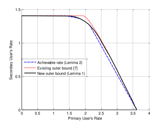
Figure 5: Comparison of new outer bound in Lemma 1 and the best existing outer bound in [7], for the GCZIC with $P_{1}=P_{2}=6,|a|=4$.

From the proof, it can be seen that without (11), optimality condition is $|\rho_{12}-\rho_{1}\rho_{2}|=\sqrt{(1-\rho_{1}^{2})(1-\rho_{2}^{2})}$ which is achieved when $h(X_{2}|U,X_{1})=0$, and implies that $X_{2}$ is a function of $(U,X_{1})$. This condition is the same as that in the inner bound. However, the inner bound applies to independent $X_{1}$ and $U$ whereas the outer bound is for general $X_{1}$ and $U$. In Section IV-D, we show that for a certain range of $a$ ($a^{2}\geq 1+P_{1}$) the optimal $X_{1}$ and $U$ for the outer bound are also independent, thus establish the capacity at that range.

Figure 5 numerically compares the outer bound proposed in Lemma 1 with the best existing outer bound in [7]. It shows that new outer bound is strictly better than the existing one. Moreover, as $|a|$ becomes larger, the gap between these two bounds increases, and the outer bound in Lemma 1 gets much closer to the achievable region. This lemma establishes the best outer bound on the capacity region of the GCZIC at strong inference ($a^{2}\geq 1$). We prove this claim by simplifying the outer bound in Lemma 1 into three simpler outer bounds in the following Corollaries. To do so, we first introduce $\alpha=1-\rho_{1}^{2},\beta=1-\rho_{2}^{2},\gamma=\rho_{12}^{2}$, $\bar{x}=1-x$, and $x\in[0,1]$ to make the bounds easier to read. These Corollaries give the capacity of the desired channel for two disjoint ranges of $a$.

Corollary 1.

Any achievable rate pair $(R_{1},R_{2})$ of the GCZIC, is upper bounded by the convex hull of the following region

$$R_{1}+R_{2} \leq\frac{1}{2}\log{\Big{(}1+P_{1}+a^{2}P_{2}+2|a|\sqrt{\gamma P_{1}P_{2}}\Big{)}}$$

$$R_{2} \leq\frac{1}{2}\log{\left(1+\bar{\gamma}P_{2}\right)}$$ (12)

where $\gamma\in[0,1]$.

This follows immediately by removing (8), (9) from the Lemma 1. This is the same as the best existing outer bound in [7], and our claim that Lemma 1 provides the best outer bound follows readily. It should be highlighted that, this region has been recently proven in [17] and [18] to be the capacity of the GCZIC for $1\leq a\leq\sqrt{1+\frac{P1}{1+P2}}$.

Corollary 2.

Any achievable rate pair $(R_{1},R_{2})$ of the GCZIC, is upper bounded by the convex hull of the following region

$$R_{2} \leq\frac{1}{2}\log{\Big{(}1+\frac{\bar{\alpha}P_{2}}{1+\alpha P_{2}}\Big{)}}$$

$$R_{1}+R_{2} \leq\frac{1}{2}\log{\Big{(}1+(\sqrt{P_{1}}+|a|\sqrt{\alpha P_{2}})^{2}\Big{)}}+\frac{1}{2}\log{\Big{(}1+\frac{\bar{\alpha}P_{2}}{1+\alpha P_{2}}\Big{)}}$$ (13)

where $\alpha\in[0,1]$.

Similar to the Corollary 1, we first eliminate (10), (11) in the Lemma 1. Then, the proof of is immediate by looking at (9), and is achieved for $\rho_{1}=0\,(\beta=1)$. As we will show later in Section IV-D, Corollary 2 is also the capacity region for the GCZIC when interference gain is considerably large ($|a|\geq\sqrt{P_{1}P_{2}}+\sqrt{1+P_{1}+P_{1}P_{2}}$).

Corollary 3.

Any achievable rate pair $(R_{1},R_{2})$ of the GCZIC, is upper bounded by the convex hull of the following region

$$R_{2} \leq\frac{1}{2}\log{\Big{(}1+\frac{\bar{\alpha}P_{2}}{1+\alpha P_{2}}\Big{)}}$$

$$R_{1}+R_{2} \leq\frac{1}{2}\log{\Big{(}1+(\sqrt{\beta P_{1}}+|a|\sqrt{\alpha P_{2}})^{2}\Big{)}}+\frac{1}{2}\log{\Big{(}1+\frac{\bar{\alpha}P_{2}}{1+\alpha P_{2}}\Big{)}}$$

$$R_{1}+R_{2} \leq\frac{1}{2}\log{\Big{(}1+P_{1}+a^{2}P_{2}+2|a|(\sqrt{\alpha\beta}+\sqrt{\bar{\alpha}\bar{\beta}})\sqrt{P_{1}P_{2}}\Big{)}}$$ (14)

where $\alpha,\beta\in[0,1]$.

To prove this, we first remove (11) in the Lemma 1. Then, in (10) we use $a\rho_{12}\leq|a||\rho_{12}|\leq|a|(|\rho_{1}\rho_{2}|+\sqrt{(1-\rho_{1}^{2})(1-\rho_{2}^{2})})$ where the last inequality follows applying triangle inequality $|x-y|\geq|x|-|y|$ with $x=\rho_{12}$ and $y=\rho_{1}\rho_{2}$ to the LHS of $|\rho_{12}-\rho_{1}\rho_{2}|\leq\sqrt{(1-\rho_{1}^{2})(1-\rho_{2}^{2})}$. The maximum is attained when $\rho_{1}\rho_{2}$ has the same sign with $a$. Finally, the outer bound in Corollary 3 is obtained considering that $\alpha\triangleq 1-\rho_{2}^{2}$, $\beta\triangleq 1-\rho_{1}^{2}$. Similar to Corollary 2, in Section IV-D, we will show that for $\beta=1$, Corollary 3 results in the capacity region of the GCZIC when $|a|\geq\sqrt{1+P_{1}}$.

IV-C Superposition coding-based inner bound for the GCZIC

In this section, we compute the Gaussian version of the achievable region introduced in Section III-A for the GCZIC. Following lemma, which extends Theorem 1 to the GCZIC, provides the achievable region by superposition coding.

Lemma 2.

Any rate pair $(R_{1},R_{2})$ satisfying

$$R_{1} \leq\frac{1}{2}\log{\left(1+(\sqrt{P_{1}}+a\sqrt{\alpha P_{2}})^{2}\right)}$$

$$R_{2} \leq\frac{1}{2}\log{\left(1+\frac{\bar{\alpha}P_{2}}{1+\alpha P_{2}}\right)}$$

$$R_{1}+R_{2} \leq\frac{1}{2}\log{\Big{(}1+P_{1}+a^{2}P_{2}+2a\sqrt{\alpha P_{1}P_{2}}\Big{)}}$$ (15)

with $\alpha\in[0,1]$ is achievable for the GCZIC.

Proof.

The achievability of this region is straightforward by Theorem 1. In the proof of Lemma 1, we have shown that jointly Gaussian input is the optimum input to maximize $I(X_{1};Y_{1}|U),I(U;Y_{2}),$ and $I(X_{1},X_{2};Y_{1})$. The cognitive user partially uses its power to help send the codewords of the primary user. $X_{2}$ contains two independent Gaussian parts, $X_{2}=\sqrt{\alpha P_{2}}V(m_{1})+\sqrt{\bar{\alpha}P_{2}}U(m_{2})$. The primary user dedicates its whole power to transmit $m_{1}$, as $X_{1}=\sqrt{P_{1}}V(m_{1})$. Decoding in the primary receiver is based on successive cancelation, where it first decode and subtract the cognitive user’s codeword in order to decode its own codeword free of interference. Cognitive receiver simply decodes its own codeword assuming the other codeword as interference. ∎

This achievable region even simplifies when the interference gain is substantially large, that is $|a|\geq\sqrt{P_{1}P_{2}}+\sqrt{1+P_{1}+P_{1}P_{2}}$. In the following section we show that, when interference is very strong ($|a|\geq\sqrt{1+P_{1}}$), the inner bound in Lemma 2 gives the capacity of the desired channel.

IV-D Capacity of the GCZIC at very strong interference

In this section, we prove that superposition coding achieves the capacity of the GCZIC for $|a|\geq\sqrt{1+P_{1}}$. Specifically, we show that in Corollary 3, $\beta$ has to be $1$ for this range of $a$. Hence, the outer bound coincides with the inner bound in Lemma 2 and gives the capacity of the desired channel.

Theorem 3.

The capacity region the GCZIC for $|a|\geq\sqrt{1+P_{1}}$ is the set of all rate pairs $(R_{1},R_{2})$ satisfying

$$R_{2} \leq\frac{1}{2}\log{\Big{(}1+\frac{\bar{\alpha}P_{2}}{1+\alpha P_{2}}\Big{)}}$$ (16)

$$R_{1}+R_{2} \leq\frac{1}{2}\log{\Big{(}1+(\sqrt{P_{1}}+|a|\sqrt{\alpha P_{2}}}\Big{)}+\frac{1}{2}\log{\Big{(}1+\frac{\bar{\alpha}P_{2}}{1+\alpha P_{2}}\Big{)}}$$ (17)

$$R_{1}+R_{2} \leq\frac{1}{2}\log{\Big{(}1+P_{1}+a^{2}P_{2}+2|a|\sqrt{\alpha P_{1}P_{2}}\Big{)}}$$ (18)

for $\alpha\in[0,1]$.

Proof.

We want to show that for $|a|\geq\sqrt{1+P_{1}}$ the outer bound in Corollary 3 and the inner bound in Lemma 2 coincide. Let’s define $\mathcal{R}_{i}$ as the set of all rate pairs satisfying the constraints in Lemma 2 and $\mathcal{R}_{o}$ as the set of all rate pairs satisfying (16)-(18). Using the same argument as El Gamal [14], we can show that $\mathcal{R}_{i}\equiv\mathcal{R}_{o}$. Here $R_{2}$ can be thought of as the rate of common message which can be decoded at both receivers while $R_{1}$ is the rate of the private message. Now $(R_{2},R_{1})\in\mathcal{R}_{o}$ if and only if $(R_{2}-t,R_{1}+t)\in\mathcal{R}_{o}$ for any $0\leq t\leq R_{2}$. This means the common rate ($R_{2}$) can be partially or entirely private. Thus region $\mathcal{R}_{o}$ can be represented as $\mathcal{R}_{i}$.

We next show that the outer bound in Corollary 3 simplifies to $\mathcal{R}_{o}$. To do so, it suffices to show that for $|a|\geq\sqrt{1+P_{1}}$, $\beta$ has to be $1$ in Corollary 3. Consider the first two inequalities of the outer bound in Corollary 3; we can see that on the boundary of this outer bound we must have

$$R_{2}\leq\frac{1}{2}\log{\Big{(}1+(\sqrt{\beta P_{1}}+|a|\sqrt{\alpha P_{2}})^{2}\Big{)}}$$ (19)

Comparing this inequality with the first inequity in $\mathcal{R}_{i}$, we conclude that either $\beta$ has to be $1$ or the first inequity of $\mathcal{R}_{i}$ must be loose; since otherwise the outer bound is less that the inner bound, which is not possible. For this inequality to be redundant in $\mathcal{R}_{i}$ we need

$$\frac{1}{2}\log{\Big{(}1+P_{1}+a^{2}P_{2}+2|a|\sqrt{\alpha P_{1}P_{2}}\Big{)}} <\frac{1}{2}\log{\left(1+\frac{\bar{\alpha}P_{2}}{1+\alpha P_{2}}\right)}+\frac{1}{2}\log{\left(1+(\sqrt{P_{1}}+|a|\sqrt{\alpha P_{2}})^{2}\right)}$$

$$\Longleftrightarrow\frac{1}{2}\log{\Big{(}1+\frac{a^{2}\bar{\alpha}P_{2}}{1+(\sqrt{P_{1}}+|a|\sqrt{\alpha P_{2}})^{2}}\Big{)}} <\frac{1}{2}\log{\left(1+\frac{\bar{\alpha}P_{2}}{1+\alpha P_{2}}\right)}$$

$$\Longleftrightarrow|a| <\sqrt{\alpha P_{1}P_{2}}+\sqrt{1+P_{1}+\alpha P_{1}P_{2}}$$ (20)

For (IV-D) to hold with any $\alpha$ then

$$|a|<\sqrt{1+P_{1}}.$$ (21)

This implies the first inequality of Lemma 2 is redundant only for $|a|<\sqrt{1+P_{1}}$. In other words, if $|a|\geq\sqrt{1+P_{1}}$ there exist some $\alpha$ for which this inequality cannot be redundant; this in turn enforces $\beta=1$. Thus, for this range of $a$, the outer bound in Corollary 3 simplifies to $\mathcal{R}_{o}$. Note also that with $\beta=1\,(\rho_{1}=0)$ the optimal input for the outer bound is the same as the input for the inner bound (i.e., $X_{1}$, $U$ are independent and $X_{2}=x_{2}(U,X_{1}$), thus the capacity is established.

∎

As a special case, when the third constraint is redundant in $\mathcal{R}_{i}$ and $\mathcal{R}_{o}$, the outer bound in Corollary 2 is tight. For such an $a$, the capacity region in Theorem 3 further simplifies as below.

Corollary 4.

The capacity region the GCZIC for $|a|\geq\sqrt{P_{1}P_{2}}+\sqrt{1+P_{1}+P_{1}P_{2}}$ is the set of all rate pairs $(R_{1},R_{2})$ satisfying

$$R_{1} \leq\frac{1}{2}\log{\Big{(}1+(\sqrt{P_{1}}+|a|\sqrt{\alpha P_{2}})^{2}\Big{)}}$$

$$R_{2} \leq\frac{1}{2}\log{\Big{(}1+\frac{\bar{\alpha}P_{2}}{1+\alpha P_{2}}\Big{)}}$$ (22)

for $\alpha\in[0,1]$.

Proof.

First consider the achievable rate region in Lemma 2. The third inequality becomes redundant if

$$\frac{1}{2}\log{\Big{(}1+P_{1}+a^{2}P_{2}+2|a|\sqrt{\alpha P_{1}P_{2}}\Big{)}} \geq\frac{1}{2}\log{\left(1+\frac{\bar{\alpha}P_{2}}{1+\alpha P_{2}}\right)}+\frac{1}{2}\log{\left(1+(\sqrt{P_{1}}+|a|\sqrt{\alpha P_{2}})^{2}\right)}$$

$$\Longleftrightarrow\frac{1}{2}\log{\Big{(}1+\frac{a^{2}\bar{\alpha}P_{2}}{1+(\sqrt{P_{1}}+|a|\sqrt{\alpha P_{2}})^{2}}\Big{)}} \geq\frac{1}{2}\log{\left(1+\frac{\bar{\alpha}P_{2}}{1+\alpha P_{2}}\right)}$$

$$\Longleftrightarrow|a| \geq\sqrt{\alpha P_{1}P_{2}}+\sqrt{1+P_{1}+\alpha P_{1}P_{2}}$$ (23)

For (IV-D) to hold with any $\alpha$ then

$$|a|\geq\sqrt{P_{1}P_{2}}+\sqrt{1+P_{1}+P_{1}P_{2}}.$$ (24)

On the other hand, without the third inequality, the achievable region in Corollary 4 is also equal to the outer bound in the Corollary 2. This is because, for the same value of $\alpha$, any point on the boundary of this region is on the boundary of the region in Corollary 2, and vice versa. Hence, we obtain the capacity region in Corollary 4 if (24) holds for any $\alpha$, i.e., $|a|\geq\sqrt{P_{1}P_{2}}+\sqrt{1+P_{1}+P_{1}P_{2}}$. ∎

Corollary 4 provides a special case of Theorem 3 with simpler rate expressions. In the concurrent and independent work [20], “Theorem V.3. Capacity for S-G-CIFC” archives the same capacity result in Corollary 4 using a different approach. The achievability follows from a more general DPC-based scheme for the Gaussian cognitive interference channel. Although the achievability seems to be based on DPC, a close observation reveals that DPC is not necessary to achieve the capacity. This is because the parameter of DPC is zero ($\lambda=0$) which means that, in effect, DPC has no contribution; thus, the achievability scheme reduces to superposition coding. The outer bound is completely different and is based on the MIMO-BC outer bound [20].

Theorem 3 shows that, when the interference is very strong, the interfered primary receiver can decode the message of the interfering cognitive transmitter in a rate higher than its own receiver. This is as though the interference link from the cognitive transmitter to the primary receiver is less noisy than the direct link for the cognitive user’s message. This sheds light on the optimal coding scheme as well. That is, the primary user encodes independently while the cognitive user encodes by superimposing the primary user’s codeword on its own. Then, the cognitive receiver decodes its message treating primary user’s codeword as noise. The primary receiver, on the other hand, performs successive cancellation; it first decodes the cognitive user’s message, then subtracts it from the received signal to decode its own message free of interference.

V Summary

Analysis of the capacity results of the GCZIC shows that superposition coding appears to be an indispensable tool in any capacity-achieving techniques for this channel. At very strong interference, superposition coding single-handedly achieves its capacity. However, both DPC and superposition coding are needed to establish the capacity when interference is weak or intermediate. Table I summarizes the capacity results for the GCZIC. As it can be seen, up to now, the capacity of this channel is characterized except for $\sqrt{1+\frac{P1}{1+P2}}<a<\sqrt{1+P_{1}}$. For this range of $a$, a more general and inclusive form of the proposed capacity-achieving outer bounds at $|a|\geq 1$, as represented in Lemma 1, provides the best outer bound on the capacity region of the GCZIC.

TABLE I: Summary of all capacity results for the GCZIC

Range of a	Capacity region	Capacity achieving	Reference
		technique
$|a|\leq 1$	$R_{1}\leq\frac{1}{2}\log{\Big{(}1+\frac{(\sqrt{P_{1}}+|a|\sqrt{\alpha P_{2}})^{2}}{1+a^{2}\bar{\alpha}P_{2}}}\Big{)}$	superposition coding	[2], [3]
	$R_{2}\leq\frac{1}{2}\log{(1+\bar{\alpha}P_{2})}$	and DPC
$1\leq|a|\leq\sqrt{1+\frac{P1}{1+P2}}$	$R_{1}+R_{2}\leq\frac{1}{2}\log{\Big{(}1+P_{1}+a^{2}P_{2}+2|a|\sqrt{\alpha P_{1}P_{2}}\Big{)}}$	superposition coding	[17], [18]
	$R_{2}\leq\frac{1}{2}\log{(1+\bar{\alpha}P_{2})}$	and DPC
$|a|>\sqrt{1+\frac{P1}{1+P2}}$	unknown	unknown	—
$|a|<\sqrt{1+P_{1}}$	(Lemma 1 gives the best outer bound)
	$R_{1}\leq\frac{1}{2}\log{\left(1+(\sqrt{P_{1}}+|a|\sqrt{\alpha P_{2}})^{2}\right)}$
$|a|\geq\sqrt{1+P1}$	$R_{2}\leq\frac{1}{2}\log{\Big{(}1+\frac{\bar{\alpha}P_{2}}{1+\alpha P_{2}}\Big{)}}$	superposition coding	Theorem [3]
	$R_{1}+R_{2}\leq\frac{1}{2}\log{\Big{(}1+P_{1}+a^{2}P_{2}+2|a|\sqrt{\alpha P_{1}P_{2}}\Big{)}}$
$|a|\geq\sqrt{P_{1}P_{2}}+\sqrt{1+P_{1}+P_{1}P_{2}}$	$R_{1}\leq\frac{1}{2}\log{\left(1+(\sqrt{P_{1}}+|a|\sqrt{\alpha P_{2}})^{2}\right)}$	superposition coding	Corollary [4],
	$R_{2}\leq\frac{1}{2}\log{\left(1+\frac{\bar{\alpha}P_{2}}{1+\alpha P_{2}}\right)}$		[20]

VI Appendix

VI-A Proof of Theorem 1

Proof.

We prove this theorem by showing the encoding, decoding, and error analysis.

VI-A1 Code construction and encoding

Fix $p(x_{1})$, $p(u)$ and $p(x_{2}|x_{1},u)$ that achieve capacity. Randomly and independently generate $2^{nR_{1}}$ sequences $x_{1}^{n}(m_{1})$, $m_{1}\in[1:2^{nR_{1}}]$ i.i.d. according to $\prod_{i=1}^{n}p(x_{1i})$. Also, randomly and independently generate $2^{nR_{2}}$ sequences $u^{n}(m_{2})$, $m_{2}\in[1:2^{nR_{2}}]$ with elements i.i.d. according to $\prod_{i=1}^{n}p_{U}(u_{i})$. Next, for each pair of sequences $(u^{n}(m_{2}),x_{1}^{n}(m_{1}))$, randomly and conditionally independently generate one sequence $x_{2}^{n}(m_{1},m_{2})$ with elements i.i.d. according to $\prod_{i=1}^{n}p_{X_{2}|X_{1}U}(x_{2i}|x_{1i}(m_{1})u_{i}(m_{2}))$.

For encoding, to send messages $(m_{1},m_{2})$, the primary transmitter just sends the codeword $x_{1}^{n}(m_{1})$ and the secondary transmitter sends the codeword $x_{2}^{n}(m_{1},m_{2})$ corresponding to those messages.

VI-A2 Decoding

Decoding is based on standard joint typicality. The less capable receiver ($Y_{2}$) can only distinguish the auxiliary random variable $U$. Decoder 2 declares that message $\hat{m}_{2}$ is sent if it is a unique message such that $(u^{n}(\hat{m}_{2}),y^{n}_{2})\in{\cal T}^{(n)}_{\epsilon}$ ; otherwise it declares an error. Decoder 1 declares that message $\hat{m}_{1}$ is sent if it is a unique message such that $(u^{n}(m_{2}),x_{1}^{n}(\hat{m}_{1}),x_{2}^{n}(\hat{m}_{1},m_{2}),y^{n}_{2})\in{\cal T}^{(n)}_{\epsilon}$ for some $m_{2}$; otherwise it declares an error.

VI-A3 Error analysis

To analyze the probability of error, without loss of generality, assume that $(M_{1},M_{2})=(1,1)$ is sent. First we consider the average probability of error for decoder 2. Let’s define the error events

$${\cal E}_{21} =(U^{n}(1),Y^{n}_{2})\notin{\cal T}^{(n)}_{\epsilon}$$

$${\cal E}_{22} =(U^{n}(m_{2}),Y^{n}_{2})\in{\cal T}^{(n)}_{\epsilon}\text{ for some }m_{2}\neq 1$$ (25)

By union bound, the probability of error for decoder 2 is upper bounded by

$${\cal E}_{2}=P({\cal E}_{21}\cup{\cal E}_{22})\leq P({\cal E}_{21})+P({\cal E}_{22}).$$ (26)

Now by law of large numbers (LLN) $P({\cal E}_{21})\rightarrow 0\text{ as }n\rightarrow\infty.$ Also, since $U^{n}(m_{2})$ is independent of $(U^{n}(1),Y^{n}_{2})$ for $m_{2}\neq 1$ by the packing lemma [19] $P({\cal E}_{22})\rightarrow 0\text{ as }n\rightarrow\infty\text{ if }R_{2}\leq I(U;Y_{2})-\delta(\epsilon).$

Then, consider the average probability of error for decoder 1. We define the following error events

$${\cal E}_{11}= (X_{1}^{n}(1),U^{n}(1),X_{2}^{n}(1,1),Y^{n}_{1})\notin{\cal T}^{(n)}_{\epsilon}$$

$${\cal E}_{12}= (X_{1}^{n}(m_{1}),U^{n}(1),X_{2}^{n}(m_{1},1),Y^{n}_{1})\in{\cal T}^{(n)}_{\epsilon}$$

$$\text{ for some }m_{1}\neq 1$$

$${\cal E}_{13}= (X_{1}^{n}(m_{1}),U^{n}(m_{2}),X_{2}^{n}(m_{1},m_{2}),Y^{n}_{1})\in{\cal T}^{(n)}_{\epsilon}$$

$$\text{ for some }m_{1}\neq 1,m_{2}\neq 1.$$ (27)

Using union bound, the probability of error for decoder 2 is upper bounded by

$${\cal E}_{2}=P({\cal E}_{11}\cup{\cal E}_{12}\cup{\cal E}_{13})\leq P({\cal E}_{11})+P({\cal E}_{12})+P({\cal E}_{13})$$ (28)

Now we evaluate each term in the right-hand side (RHS) of this inequality when $n\rightarrow\infty$. First consider ${\cal E}_{11}$; again by LLN $P({\cal E}_{11})\rightarrow 0\text{ as }n\rightarrow\infty.$ Next consider ${\cal E}_{12}$. For $m_{1}\neq 1$ since $(X_{1}(m_{1}),X_{2}(m_{1},1))$ is conditionally independent of $Y^{n}_{1}$ given $U^{n}(1)$, by packing lemma $P({\cal E}_{12})\rightarrow 0\text{ as }n\rightarrow\infty\text{ given }R_{1}\leq I(X_{1},X_{2};Y_{1}|U)-\delta(\epsilon)=I(X_{1};Y_{1}|U)-\delta(\epsilon)$ because $X_{2}$ is a function of $(U,X_{1})$. Finally consider ${\cal E}_{13}$. For $m_{1}\neq 1$ and $m_{2}\neq 1$, $(X_{1}(m_{1}),U^{n}(m_{2}),X_{2}(m_{1},m_{2}))$ is independent of $Y^{n}_{1}$; hence, by packing lemma $P({\cal E}_{13})\rightarrow 0\text{ as }n\rightarrow\infty\text{ if }R_{1}+R_{2}\leq I(X_{1},U,X_{2};Y_{1})-\delta(\epsilon)=I(X_{1},X_{2};Y_{1})-\delta(\epsilon)$. The equality follows because $U\rightarrow X_{1},X_{2}\rightarrow Y_{1}$ forms a Markov chain. The above analysis completes the proof of achievability since it shows that both receivers can decode corresponding messages with the total probability of error tending to zero if (4) is satisfied. Therefore, there exists a sequence of codes with error probability tending to 0. ∎

VI-B Proof of Theorem 2

VI-B1 For more capable DM-CIC

The proof is also similar to the converse proof for the more capable broadcast channel [14]. We follow the same line of proof as in [19]; the only difference is replacing $X_{1}$ in [19] with $(X_{1},X_{2})$, since here $X_{2}$ also encodes $M_{1}$.

We can bound the rates $R_{2}$ and $R_{2}+R_{2}$ as

$$nR_{2} =H(M_{2})$$

$$=I(M_{2};Y^{n}_{2})+H(M_{2}|Y^{n}_{2})$$

$$\leq I(M_{2};Y^{n}_{2})+n\epsilon_{1n}$$ (29)

and

$$n(R_{1}+R_{2}) =H(M_{1},M_{2})$$

$$=H(M_{1}|M_{2})+H(M_{2})$$

$$=I(M_{1};Y^{n}_{1}|M_{2})+H(M_{1}|Y^{n}_{1},M_{2})+I(M_{2};Y^{n}_{2})+H(M_{2}|Y^{n}_{2})$$

$$\leq I(M_{1};Y^{n}_{1}|M_{2})+I(M_{2};Y^{n}_{2})+n\epsilon_{2n}$$ (30)

where (29) and (30) follow by Fano’s inequality. In a very similar fashion, sum rate can be also bounded by

$$n(R_{1}+R_{2}) \leq I(M_{2};Y^{n}_{2}|M_{1})+I(M_{1};Y^{n}_{1})+n\epsilon_{3n}.$$ (31)

Now we manipulate the RHS of (29)-(31) to obtain the desired terms in (5). First, consider the mutual information term in (29)

$$I(M_{2};Y^{n}_{2}) =\sum^{n}_{\begin{subarray}{c}i=1\end{subarray}}I(M_{2};Y_{2i}|Y^{n}_{2,i+1})$$ (32)

$$\leq\sum^{n}_{\begin{subarray}{c}i=1\end{subarray}}I(M_{2},Y^{n}_{2,i+1};Y_{2i})$$

$$\leq\sum^{n}_{\begin{subarray}{c}i=1\end{subarray}}I(M_{2},Y^{i-1}_{1},Y^{n}_{2,i+1};Y_{2i})$$

$$=\sum^{n}_{\begin{subarray}{c}i=1\end{subarray}}I(U_{i};Y_{2i})$$ (33)

in which (32) follows from the chain rule, and we have defined the auxiliary random variable $U_{i}=(M_{2},Y^{i-1}_{1},Y^{n}_{2,i+1})$ moving to (VI-B1). Next, we bound the mutual information terms of the second inequality in (30).

$$I(M_{1};Y^{n}_{1}|M_{2})+I(M_{2};Y^{n}_{2})= \sum^{n}_{\begin{subarray}{c}i=1\end{subarray}}I(M_{1};Y_{1i}|M_{2},Y^{i-1}_{1})+\sum^{n}_{\begin{subarray}{c}i=1\end{subarray}}I(M_{2};Y_{2i}|Y^{n}_{2,i+1})$$

$$\leq \sum^{n}_{\begin{subarray}{c}i=1\end{subarray}}I(M_{1},Y^{n}_{2,i+1};Y_{1i}|M_{2},Y^{i-1}_{1})+\sum^{n}_{\begin{subarray}{c}i=1\end{subarray}}I(M_{2},Y^{n}_{2,i+1};Y_{2i})$$

$$= \sum^{n}_{\begin{subarray}{c}i=1\end{subarray}}I(M_{1},Y^{n}_{2,i+1};Y_{1i}|M_{2},Y^{i-1}_{1})$$

$$+\sum^{n}_{\begin{subarray}{c}i=1\end{subarray}}I(M_{2},Y^{n}_{2,i+1},Y^{i-1}_{1};Y_{2i})-\sum^{n}_{\begin{subarray}{c}i=1\end{subarray}}I(Y^{i-1}_{1};Y_{2i}|M_{2},Y^{n}_{2,i+1})$$

$$= \sum^{n}_{\begin{subarray}{c}i=1\end{subarray}}I(M_{1};Y_{1i}|M_{2},Y^{i-1}_{1},Y^{n}_{2,i+1})+\sum^{n}_{\begin{subarray}{c}i=1\end{subarray}}I(M_{2},Y^{n}_{2,i+1},Y^{i-1}_{1};Y_{2i})$$

$$-\sum^{n}_{\begin{subarray}{c}i=1\end{subarray}}I(Y^{i-1}_{1};Y_{2i},|M_{2},Y^{n}_{2,i+1})+\sum^{n}_{\begin{subarray}{c}i=1\end{subarray}}I(Y^{n}_{2,i+1};Y_{1i},|M_{2},Y^{i-1}_{1})$$

$$= \sum^{n}_{\begin{subarray}{c}i=1\end{subarray}}I(M_{1};Y_{1i}|U_{i})+\sum^{n}_{\begin{subarray}{c}i=1\end{subarray}}I(U_{i};Y_{2i})$$ (34)

$$\leq \sum^{n}_{\begin{subarray}{c}i=1\end{subarray}}I(X_{1i};Y_{1i}|U_{i})+\sum^{n}_{\begin{subarray}{c}i=1\end{subarray}}I(U_{i};Y_{2i})$$ (35)

where (34) follows by the Csiszar sum identity and the auxiliary random variable $U_{i}=(M_{2},Y^{i-1}_{1},Y^{n}_{2,i+1})$; (35) follows by Markov chain $M_{1}\rightarrow(X_{1}U)\rightarrow Y_{1}$.

For the third inequality, following steps similar to the bound for the second inequality and defining $V_{i}:=(M_{1},Y^{i-1}_{1},Y^{n}_{2,i+1})$ we can bound the mutual information terms in (31) as

$$I(M_{2};Y^{n}_{2}|M_{1})+I(M_{1};Y^{n}_{1}) =\sum^{n}_{\begin{subarray}{c}i=1\end{subarray}}I(M_{2};Y_{2i}|M_{1},Y_{2}^{i-1})+\sum^{n}_{\begin{subarray}{c}i=1\end{subarray}}I(M_{1};Y_{2i}|Y_{2}^{i-1})$$

$$\leq\sum^{n}_{\begin{subarray}{c}i=1\end{subarray}}I(M_{2};Y_{2i}|V_{i})+\sum^{n}_{\begin{subarray}{c}i=1\end{subarray}}I(V_{i};Y_{2i})$$ (36)

$$\leq\sum^{n}_{\begin{subarray}{c}i=1\end{subarray}}I(X_{1i},X_{2i};Y_{2i}|V_{i})+\sum^{n}_{\begin{subarray}{c}i=1\end{subarray}}I(V_{i};Y_{1i})$$ (37)

$$\leq\sum^{n}_{\begin{subarray}{c}i=1\end{subarray}}I(X_{1i},X_{2i};Y_{1i}|V_{i})+\sum^{n}_{\begin{subarray}{c}i=1\end{subarray}}I(V_{i};Y_{1i})$$ (38)

$$=\sum^{n}_{\begin{subarray}{c}i=1\end{subarray}}I(X_{1i},X_{2i};Y_{1i})$$

in which (36) follows similar steps to the bound for the first inequality on sum rate; (37) follows from $M_{2}\rightarrow X_{1},X_{2}\rightarrow Y_{2}$; and (38) follows by (2) that gives $I(X_{1},X_{2};Y_{1})\geq I(X_{1},X_{2};Y_{2})$, and implies that $I(X_{1},X_{2};Y_{2}|V)\leq I(X_{1},X_{2};Y_{1}|V)$.

Next, we define the time sharing random variable $Q$ which is uniformly distributed over $[1:n]$ and is independent of $(M_{1},M_{2},X^{n}_{1},X^{n}_{2},Y^{n}_{1},Y^{n}_{2})$. Also we define $U=(Q,U_{Q}),X^{n}_{1}=X^{n}_{1Q},X^{n}_{2}=X^{n}_{2Q},Y^{n}_{1}=Y^{n}_{1Q},Y^{n}_{2}=Y^{n}_{2Q}$. Then we have

$$nR_{2} \leq\sum^{n}_{\begin{subarray}{c}i=1\end{subarray}}I(U_{i};Y_{2i})+n\epsilon_{1n}$$

$$=nI(U;Y_{2}|Q)+n\epsilon_{1n}$$

$$\leq nI(U;Y_{2})+n\epsilon_{1n}$$

Similarly

$$n(R_{1}+R_{2}) \leq\sum^{n}_{\begin{subarray}{c}i=1\end{subarray}}I(X_{1i};Y_{1i}|U_{i})+\sum^{n}_{\begin{subarray}{c}i=1\end{subarray}}I(U_{i};Y_{2i})+n\epsilon_{2n}$$

$$=nI(X_{1};Y_{1}|U,Q)+nI(U;Y_{2}|Q)+n\epsilon_{2n}$$

$$=nI(X_{1};Y_{1}|U)+nI(U;Y_{2}|Q)+n\epsilon_{2n}$$

$$\leq nI(X_{1};Y_{1}|U)+nI(U;Y_{2})+n\epsilon_{2n}$$

and

$$n(R_{1}+R_{2}) \leq\sum^{n}_{\begin{subarray}{c}i=1\end{subarray}}I(X_{1i},X_{2i};Y_{1i})+n\epsilon_{3n}.$$

$$=nI(X_{1},X_{1};Y_{1}|Q)+n\epsilon_{3n}$$

$$\leq nI(X_{1},X_{1};Y_{1})+n\epsilon_{3n}$$

As $n\rightarrow\infty$, $\epsilon_{1n},\epsilon_{2n},$ and $\epsilon_{3n}$ tend to zero because the probability of error is assumed to vanish. This completes the proof for the more capable DM-CIC.

VI-B2 For DM-CIC with strong interference

Proof.

The proof outer bound under the strong interference condition (3) is almost the same, with only slight difference in the proof of last inequality. This is because the first two inequalities hold for any DM-CIC. Under the strong interference condition (3) we can we can bound the mutual information terms in (31) as

$$I(M_{2};Y^{n}_{2}|M_{1})+I(M_{1};Y^{n}_{1}) \leq I(M_{2};Y^{n}_{2}|M_{1},X^{n}_{1})+I(M_{1},X^{n}_{1};Y^{n}_{1})$$

$$\leq I(X^{n}_{2};Y^{n}_{2}|M_{1},X^{n}_{1})+I(M_{1},X^{n}_{1};Y^{n}_{1})$$

$$\leq I(X^{n}_{2};Y^{n}_{1}|M_{1},X^{n}_{1})+I(M_{1},X^{n}_{1};Y^{n}_{1})$$ (39)

$$=I(X^{n}_{1},X^{n}_{2};Y^{n}_{1})$$

$$\leq\sum^{n}_{\begin{subarray}{c}i=1\end{subarray}}I(X_{1i},X_{2i};Y_{1i})$$

in which (39) follows by (3) that gives $I(X_{2};Y_{2}|X_{1})\leq I(X_{2};Y_{1}|X_{1})$, and implies that $I(X_{2};Y_{2}|X_{1},M_{1})\leq I(X_{2};Y_{1}|X_{1},M_{1})$. The other steps are straightforward. Finally, this proves that Theorem 2 holds both for more capable strong and interference DM-CIC. ∎

VI-C Proof of Lemma 1

Proof.

We need to find the distribution that maximize the rate region in Theorem 2 for the Gaussian channel. In what follows, we show that jointly Gaussian $X_{1},X_{2},U$ is optimum, i.e., it provides the largest outer bound for the Gaussian channel. By maximum entropy theorem, the RHS of the third inequality is maximized when $Y_{1}$ is Gaussian, thus $Y_{1}=X_{1}+aX_{2}+Z_{1}\text{ is Gaussian; that is }X_{1}+aX_{2}\text{ must be Gaussian. }$

Similarly,

$$R_{2} \leq I(U;Y_{2})$$

$$=h(Y_{2})-h(Y_{2}|U)$$

$$\leq h(Y_{2}^{G})-h(Y_{2}|U)$$

$$\leq h(Y_{2}^{G})-\frac{1}{2}\log\left({2^{2h(X_{2}|U)}+2^{2h(Z_{2})}}\right)$$ (40)

where $Y_{2}^{G}$ denotes $Y_{2}$ when the inputs $X_{1},X_{2}$ are Gaussian. The last inequality follows by conditional version of entropy power inequality (EPI) for which equality is achieved when $X_{2}|U\text{ is Gaussian }$. Likewise, for the term $I(X_{1};Y_{1}|U)$ we can write

$$I(X_{1};Y_{1}|U) =h(Y_{1}|U)-h(Y_{1}|U,X_{1})$$

$$\leq h(X_{1}^{G}|U^{G}+aX_{2}^{G}|U^{G}+Z_{1})-h(Y_{1}|U,X_{1})$$

$$\leq h(X_{1}^{G}|U^{G}+aX_{2}^{G}|U^{G}+Z_{1})-\frac{1}{2}\log\left({2^{2h(aX_{2}|U,X_{1})}+2^{2h(Z_{2})}}\right)$$

where where $X_{1}^{G},U^{G}$ denote$X_{1},U$ when the inputs $X_{1},X_{2}$ are Gaussian, and inequalities follow by maximum entropy theorem and conditional version of EPI, respectively. Again equality is achieved when all terms are Gaussian. Hence, all inequalities in the outer bound are maximized with jointly Gaussian $X_{1},X_{2},U$.

Now the problem is to find the optimum covariance matrix to maximize the bounds, i.e., to determine correlation coefficients among $X_{1},X_{2},$ and $U$. Let $(U,X_{1},X_{2})\sim{\cal N}(0,K)$, which are correlated Gaussian random variables $X_{1},X_{2},$ and $U$ with covariance matrix

$$K=COV(U,X_{1},X_{2})=\left(\begin{array}[]{ccccccc}P_{U}&\rho_{1}\sqrt{P_{U}P_{1}}&\rho_{2}\sqrt{P_{U}P_{2}}\\ \rho_{1}\sqrt{P_{U}P_{1}}&P_{1}&\rho_{12}\sqrt{P_{1}P_{2}}\\ \rho_{2}\sqrt{P_{U}P_{2}}&\rho_{12}\sqrt{P_{1}P_{2}}&P_{2}\\ \end{array}\right)$$ (44)

Since the covariance matrix is positive semidefinite, the determinant of this matrix must be nonnegative. That is

$$1-\rho_{12}^{2}-\rho_{1}^{2}+2\rho_{1}\rho_{2}\rho_{12}-\rho_{2}^{2}\geq 0.$$ (45)

The inequality holds if

$$\rho_{1}\rho_{2}-\sqrt{(1-\rho_{1}^{2})(1-\rho_{2}^{2})}\leq\rho_{12}\leq\rho_{1}\rho_{2}+\sqrt{(1-\rho_{1}^{2})(1-\rho_{2}^{2})}$$

or equivalently the covariance matrix is positive semidefinite if

$$|\rho_{12}-\rho_{1}\rho_{2}|\leq\sqrt{(1-\rho_{1}^{2})(1-\rho_{2}^{2})}.$$ (46)

Now we evaluate the rate constraints defining the outer bound in Theorem 2.

$$R_{2} \leq I(U;Y_{2})$$

$$=h(Y_{2})+h(U)-h(Y_{2},U)$$

$$=h(X_{2}+Z_{2})+h(U)-h(X_{2}+Z_{2},U)$$

$$=\frac{1}{2}\log{2\pi e\left(1+P_{2}\right)}+\frac{1}{2}\log{2\pi e\left(P_{U}\right)}-\frac{1}{2}\log{(2\pi e)^{2}|K_{1}|}$$

$$=\frac{1}{2}\log{\left(\frac{1+P_{2}}{1+P_{2}(1-\rho_{2}^{2})}\right)}$$ (47)

where

$$K_{1}=\left(\begin{array}[]{cc}1+P_{2}&\rho_{2}\sqrt{P_{U}P_{2}}\\ \rho_{2}\sqrt{P_{U}P_{2}}&P_{U}\\ \end{array}\right)$$

Similarly

$$I(X_{1};Y_{1}|U) =h(Y_{1}|U)-h(Y_{1}|U,X_{1})$$

$$=h(Y_{1},U)-h(U)-\frac{1}{2}\log\left({2^{2h(aX_{2}|U,X_{1})}+2^{2h(Z_{1})}}\right)$$

$$\leq h(Y_{1},U)-h(U)-\frac{1}{2}\log\left({2^{2h(Z_{1})}}\right)$$ (48)

$$=\frac{1}{2}\log{\left(|K_{2}|/P_{U}\right)}$$

where

$$|K_{2}| =\left|\left(\begin{array}[]{cc}1+P_{1}+a^{2}P_{2}+2a\rho_{12}\sqrt{P_{1}P_{2}}&\rho_{1}\sqrt{P_{U}P_{1}}+a\rho_{2}\sqrt{P_{U}P_{2}}\\ \rho_{1}\sqrt{P_{U}P_{1}}+a\rho_{12}\sqrt{P_{U}P_{2}}&P_{U}\\ \end{array}\right)\right|$$ (51)

$$=P_{U}(1+P_{1}+a^{2}P_{2}+2a\rho_{12}\sqrt{P_{1}P_{2}}-\rho_{1}^{2}P_{1}-a^{2}\rho_{2}^{2}P_{2}-2a\rho_{1}\rho_{2}\sqrt{P_{1}P_{2}})$$

To check if the inequality (48) can hold with equality, we evaluate the term $2^{2h(aX_{2}|U,X_{1})}$

$$h(X_{2}|U,X_{1}) =h(U,X_{1},X_{2})-h(U,X_{1})$$

$$=\frac{1}{2}\log\left((2\pi e)^{3}|K|\right)-\frac{1}{2}\log{\left((2\pi e)^{2}P_{U}P_{1}(1-\rho_{1}^{2})\right)}$$

$$=\frac{1}{2}\log{2\pi eP_{2}\left(\frac{1-\rho_{12}^{2}-\rho_{1}^{2}-\rho_{2}^{2}+2\rho_{12}\rho_{2}\rho_{1}}{1-\rho_{1}^{2}}\right)}$$ (52)

in which the covariance matrix $K$ is defined by (44). Since both numerator and denominator are nonnegative in (48), the argument of this function is either zero or positive. Therefore, $\min({2^{2h(aX_{2}|U,X_{1})}})=0$ is achieved when $1-\rho_{12}^{2}-\rho_{1}^{2}-\rho_{2}^{2}+2\rho_{12}\rho_{2}\rho_{1}=0$, or equivalently, $|\rho_{12}-\rho_{1}\rho_{2}|=\sqrt{(1-\rho_{1}^{2})(1-\rho_{2}^{2})}$. Note that $h(aX_{2}|U,X_{1})=0$ implies $X_{2}$ to be a function of $(U,X_{1})$.

Keeping this in mind that $|\rho_{12}-\rho_{1}\rho_{2}|=\sqrt{(1-\rho_{1}^{2})(1-\rho_{2}^{2})}$ is optimum condition for (48), we evaluate $I(X_{1};Y_{1}|U)$ as follows.

$$I(X_{1};Y_{1}|U) \leq\frac{1}{2}\log{\left(|K_{2}|/P_{U}\right)}$$

$$=\frac{1}{2}\log{\left(1+(1-\rho_{1}^{2})P_{1}+a^{2}(1-\rho_{2}^{2})P_{2}+2a(\rho_{12}-\rho_{1}\rho_{2})\sqrt{P_{1}P_{2}}\right)}$$

$$\leq\frac{1}{2}\log{\left(1+(1-\rho_{1}^{2})P_{1}+a^{2}(1-\rho_{2}^{2})P_{2}+2|a||\rho_{12}-\rho_{1}\rho_{2}|\sqrt{P_{1}P_{2}}\right)}$$

$$\leq\frac{1}{2}\log{\left(1+(1-\rho_{1}^{2})P_{1}+a^{2}(1-\rho_{2}^{2})P_{2}+2|a|\sqrt{(1-\rho_{1}^{2})(1-\rho_{2}^{2})P_{1}P_{2}}\right)}$$

where, the last inequality follows from (46). Interestingly, again

$$|\rho_{12}-\rho_{1}\rho_{2}|=\sqrt{(1-\rho_{1}^{2})(1-\rho_{2}^{2})}$$ (53)

turns out to be the optimum condition. From this two values for $\rho_{12}$ are plausible which are respectively

$$\rho_{12}^{(1)}=\rho_{1}\rho_{2}+\sqrt{(1-\rho_{1}^{2})(1-\rho_{2}^{2})}$$ (54)

$$\rho_{12}^{(2)}=\rho_{1}\rho_{2}-\sqrt{(1-\rho_{1}^{2})(1-\rho_{2}^{2})}$$ (55)

Then, it is also straightforward to calculate the third bound in Theorem 2 to obtain

$$R_{1}+R_{2} \leq\frac{1}{2}\log{\left(1+P_{1}+a^{2}P_{2}+2a\rho_{12}\sqrt{P_{1}P_{2}}\right)}$$

$$\leq\frac{1}{2}\log{\left(1+P_{1}+a^{2}P_{2}+2\max\{a\rho_{12}^{(1)},a\rho_{12}^{(2)}\}\sqrt{P_{1}P_{2}}\right)}$$

Therefore, from the outer bound in Theorem 2, we compute the rate region $\mathcal{R}_{\mathbb{G}}$ with following constraints

$$R_{2} \leq\frac{1}{2}\log{\left(\frac{1+P_{2}}{1+P_{2}(1-\rho_{2}^{2})}\right)}$$

$$R_{1}+R_{2} \leq\frac{1}{2}\log{\left(1+(1-\rho_{1}^{2})P_{1}+a^{2}(1-\rho_{2}^{2})P_{2}+2|a|\sqrt{(1-\rho_{1}^{2})(1-\rho_{2}^{2})P_{1}P_{2}}\right)}$$

$$+\frac{1}{2}\log{\left(\frac{1+P_{2}}{1+P_{2}(1-\rho_{2}^{2})}\right)}$$

$$R_{1}+R_{2} \leq\frac{1}{2}\log{\left(1+P_{1}+a^{2}P_{2}+2\max\{a\rho_{12}^{(1)},a\rho_{12}^{(2)}\}\sqrt{P_{1}P_{2}}\right)}$$

As a last step, we can evaluate and add the Gaussian version of the standard inequality $R_{2}\leq I(X_{2};Y_{2}|X_{1})$ [3], [4], to these bounds; the corresponding inequality is

$$R_{2} \leq\frac{1}{2}\log{\left(1+(1-\rho_{12}^{2})P_{2}\right)}$$ (56)

As a result, the outer bound is as given in Lemma 1. ∎

References

• [1] N. Devroye, P. Mitran, and V. Tarokh, β€œAchievable Rates in Cognitive Channels,” IEEE Transactions on Information Theory, vol. 52, no. 5, pp. 1813-1827, May 2006.
• [2] A. Jovicic and P. Viswanath, β€œCognitive Radio: An Information- Theoretic Perspective,” in Proc. IEEE Int. Symp. Inf. Theory, July 2006, pp. 2413-2417.
• [3] W. Wu, S. Vishwanath, and A. Arapostathis, β€œCapacity of a Class of Cognitive Radio Channels: Interference Channels With Degraded Message Sets,” IEEE Transactions on Information Theory, vol. 53, no. 11, pp. 4391-4399, Nov. 2007.
• [4] I. Maric, R. Yates, and G. Kramer, β€œThe strong interference channel with unidirectional cooperation,” in Information Theory and Applications ITA Inaugural Workshop, Feb. 2006.
• [5] J. Jiang and Y. Xin, β€œOn the Achievable Rate Regions for Interference Channels With Degraded Message Sets,” IEEE Transactions on Information Theory, vol. 54, no. 10, pp. 4707-4712, Oct. 2008.
• [6] I. Maric, R. Yates, and G. Kramer, β€œCapacity of interference channels with partial taransmitter cooperation,” IEEE Trans. Inf. Theory, vol. 53, no. 10, pp. 3536-3548, October 2007.
• [7] I. Maric, A. Goldsmith, G. Kramer, and S. Shamai (Shitz), β€œOn the capacity of interference channels with one cooperatig taransmitter,” European Trans. Telecomm., vol. 19, no. 10, pp. 405-420, April 2008.
• [8] M. H. M. Costa, β€œWriting on dirty paper,” IEEE Transactions on Information Theory, vol. 29, no. 3, pp. 439-441, May 1983.
• [9] T. M. Cover, and J. A. Thomas, Elements of Information Theory, New York: John Wiley & Sons, 1991.
• [10] T. Han and K. Kobayashi, β€œA new achievable rate region for the interference channel,” IEEE Transactions on Information Theory, vol. IT-27, no. 1, pp. 49-60, 1981.
• [11] S. Gel fand and M. Pinsker, β€œCoding for channels with random parameters,” Problems of Control and Information Theory, vol. 9, no. 1, pp. 19-31, 1980.
• [12] A. Carleial, β€œInterference channels,” IEEE Transactions on Information Theory, vol. IT-24, no. 1, pp. 60-70, Jan. 1978.
• [13] G. Kramer, β€œReview of rate regions for interference channels,” in Proc. 2006 Int. Zurich Seminar on Communications, Zurich, Switzerland, pp. 162-165, Feb. 2006.
• [14] A. El Gamal, β€œThe capacity of a class of broadcast channels,” IEEE Trans. on Inf. Theory, vol. 25, no. 2, pp. 166-169, 1979.
• [15] N. Liu, I. Maric, A. Goldsmith and Shlomo Shamai (Shitz), β€œBounds and Capacity Results for the Cognitive Z-interference channel,” in Proc. IEEE Int. Symp. Inf. Theory, (ISIT09), Seoul, Korea, June 2009.
• [16] Y. Cao and B. Chen, β€œThe Cognitive Z Channel,” in Proc. IEEE Global Comm. Conference (GLOBECOM 2009), Hawaii, USA, pp. 528-532, Nov. 2009.
• [17] S. Rini, D. Tuninetti and N. Devroye, β€œNew Results on the Capacity of the Gaussian Cognitive Interference Channel,” Forty-Eighth Annual Allerton Conference on Communication, Control, and Computing, Monticello, Sept. 2010.
• [18] J. Jiang, I. Maric, A. Goldsmith, S. Shamai (Shitz), S. Cui, β€œOn the Capacity of a Class of Cognitive Z-interference Channels,” submitted to ICC2011, available at http://arxiv.org/abs/1007.1811.
• [19] A. El Gamal and Y. H. Kim, Lecture Notes on Network Information Theory, available at http://arxiv.org/abs/1001.3404.
• [20] S. Rini, D. Tuninetti and N. Devroye, β€œInner and Outer Bounds for the Gaussian Cognitive Interference Channel and New Capacity Results,” submitted to IEEE Trans. on Inf. Theory, October 2010, available at http://arxiv.org/abs/1010.5806.