Quantum theory of the electromagnetic response of metal nanofilms

Abstract

We develop a quantum theory of electron confinement in metal nanofilms. The theory is used to compute the nonlinear response of the film to a static or low-frequency external electric field and to investigate the role of boundary conditions imposed on the metal surface. We find that the sign and magnitude of the nonlinear polarizability depends dramatically on the type of boundary condition used.

I Introduction

The recent explosion of growth in the field of nanoplasmonics Maier et al. (2003); Prodan et al. (2003); Stockman (2008a, b); Brongersma and Shalaev (2010) have been a joint success of theory and experiment. Yet, in certain respects, theory is lagging behind. One profound theoretical question, which has not received adequate attention so far, is related to the applicability of macroscopic theories. That is, the theory of plasmonic systems is almost exclusively based on the macroscopic Maxwell’s equations, even though the samples involved are, in some cases, only a few nanometers in size. The problem is compounded by the fact that plasmonic applications utilize highly conductive noble metals. In this case, the mean free path of the conduction electrons, which can be significantly larger than interatomic distances, becomes of primary importance. Several different approaches to accounting for the finite-size and quantum effects in nanoparticles have been proposed Halas et al. (2011). However, finite-size-dependent electromagnetic nonlinearities have received relatively little attention. In this paper, we theoretically investigate finite-size effects in metallic nanofilms with an emphasis on electromagnetic nonlinearity and on the role of boundary conditions applied at the nanofilm surface.

A qualitative understanding of finite-size effects in plasmonic systems can be gained from purely classical arguments. For example, it has been demonstrated that the electromagnetic response of a strongly coupled plasmonic system is dramatically altered by the effects of nonlocality when the smallest geometrical feature of the system (e.g., an interparticle gap) becomes comparable to a certain phenomenological length scale, which characterizes the intrinsic nonlocality of metal Dasgupta and Fuchs (1981); Fuchs and Claro (1987); Ruppin (1992). A qualitative theory of optical nonlinearity can also be derived from purely classical arguments Panasyuk et al. (2008).

However, a quantitatively accurate theory must be quantum mechanical. Unfortunately, a fully self-consistent and mathematically-tractable quantum model of plasmonic systems is difficult to formulate. In Refs. Hache et al., 1986; Rautian, 1997, a metal nanosphere was approximated by a degenerate electron gas confined in a spherical, infinitely-high potential well. The conduction electrons were assumed to be driven by a time-harmonic and spatially-uniform electric field. This driving field is internal to the nanoparticle; relating it to the external (applied) field constitutes a separate problem Drachev et al. (2004). The model of Refs. Hache et al., 1986; Rautian, 1997 has attracted considerable attention in the optics community. In particular, it predicts correctly the size dependence of the Drude relaxation constant. Although the model is mathematically tractable, it yields an expression for the third-order nonlinear polarizability, which involves an eight-fold series. This expression can be evaluated only approximately Rautian (1997). Recently, we have reduced analytically this expression (without resorting to any additional approximations) to a five-fold series, which is amenable to direct numerical evaluation Govyadinov et al. (2001). We then have used this result to study the size- and frequency dependence of the third-order nonlinear polarizability.

Still, formulation of the model of Refs. Hache et al., 1986; Rautian, 1997 involves two important assumptions, which are difficult to avoid and whose effect is difficult to predict. First, the model assumes a spatially-uniform electric field inside the nanoparticle. In reality, this field is not spatially-uniform because the induced charge density is different from the infinitely-thin surface density of the Lorenz-Lorentz theory, which was used in Refs. Rautian, 1997; Drachev et al., 2004 and also by us Govyadinov et al. (2001) to obtain a relation between the internal and the applied fields. A relation of this kind is essential for deriving any experimentally-measurable quantity. Unfortunately, a more fundamental approach to relating the internal and applied fields does not readily present itself, at least, not within the formalism of Refs. Hache et al., 1986; Rautian, 1997. Second, the imposition of an infinite potential barrier at the nanoparticle surface has not been justified from first principles, even though this boundary condition is frequently employed and can be defended by noting that a gas of noninteracting electrons can not be stably bound by the Coulomb potential of a spatially-uniform, positively-charged background. In other words, the potential barrier makes up for the neglect of the discrete nature of positively-charged ions.

The two assumptions described above can be, in principle, avoided by using the density-functional theory (DFT). Within DFT, the exchange-correlation potential renders the system stable even if the ionic lattice is replaced by jellium. Time dependent DFT (TDDFT) and the jellium model have been successfully used to compute the linear response of nanoparticles Ekardt (1984); Lerme et al. (1999). TDDFT and the random-phase approximation (RPA) have been used without resorting to jellium model (that is, with the full account of crystalline structure of metal) to study the effects of surface molecular adsorption on the dielectric losses in metal Zhu et al. (2008); Gavrilenko et al. (2010). Size- and shape-dependence of the imaginary part of the dielectric function of Ag nanoparticles has been also studied experimentally Drachev et al. (2008); Qiu et al. (2008).

However, it is not clear whether the same DFT-based approaches are appropriate for obtaining nonlinear corrections to the polarizability. Indeed, the exchange-correlation potential is typically constructed for an infinite and spatially-uniform system and is not expected to be accurate near boundaries, where the electron density changes on small spatial scales. Yet, it can be argued that the nonlinear response of a nanoparticle is strongly influenced by the electron density near the boundary Panasyuk et al. (2008). Further, if the jellium model is used, as is the case in this work, the binding potential of the positively-charged jellium (even with the account of exchange-correlation potential) is not as strong as that of discrete ionic lattice. In the latter case, the Coulomb potential approaches negative infinity in the vicinity of the ion cores. Therefore, it is not evident whether the correct model should incorporate an additional potential barrier at the surface of the nanoparticle to account phenomenologically for the reduced binding power of the jellium. Considering the above uncertainty, and the fact that the infinite potential barrier of Ref. Rautian, 1997; Drachev et al., 2004 has been widely used in the optics literature, it seems desirable to investigate the influence of the boundary conditions used on the obtained nonlinear corrections.

To address the problem formulated above, we have performed DFT calculations for the simplest plasmonic system – a thin metallic film to which a static or low-frequency perpendicularly-polarized electric field is applied. We have investigated the influence of three different types of boundary conditions, including the rigid (infinite potential barrier) boundary condition, the Bardeen’s boundary condition (in which the potential barrier is displaced from the metal surface) and free boundaries. We compute nonlinear corrections to the film polarizability by two different approaches – first, by the use of a perturbation theory, which is described in detail below and, second, by direct numerical application of the DFT (for control). For relatively strong applied fields, when the perturbation theory is not applicable, the nonlinear polarization is computed directly by DFT.

The paper is organized as follows. In Sec. II we describe the physical model in more detail. In Sec. III, we write the basic equations of the DFT and specialize them to the thin film problem. The perturbation theory is described in Sec. IV. Numerical results are reported in Sec. V. Finally, Sec. VI contains a summary and a discussion.

II The physical model

Throughout this paper we consider the following model system. A thin metallic film of width $h$ is taken to occupy the spatial region $-L/2<x,y<L/2$, $-h/2<z<h/2$, where $L\gg h$. The latter condition allows for the neglect of effects due to the edges of the slab. Accordingly, we assume that all physical quantities depend only on the variable $z$, so that the system is effectively one-dimensional. A static electric field of strength ${\mathscr{E}}$ is applied to the slab in the $z$-direction. We emphasize that this is the external (applied) field; not the internal field of Refs. Hache et al., 1986; Rautian, 1997.

We use the stabilized jellium model Shore and Rose (1991); Perdew et al. (1990); Liebsch (1997) and the Gunnarsson-Lundqvist local-density approximation for the exchange-correlation potential Gunnarsson and Lundqvist (1976) (defined precisely below). At or near the film surface, we apply three different types of boundary conditions. In our first set of calculations, we apply the infinite potential wall condition of Refs. Hache et al., 1986; Rautian, 1997 at the physical boundary of metal. We denote this type of boundary condition by “R” (in memory of S.G.Rautian Rautian (1997)). In a second set of calculations, employing what we refer to as the “B”-type boundary condition, we use the classical Bardeen model Bardeen (1936); Pitarke and Eguiluz (2001); Han and Liu (2009) in which the potential wall is displaced from the physical boundary by the distance

$$\Delta_{\rm B}=\frac{3\pi}{8k_{\rm F}}\ ,$$ (1)

where $k_{\rm F}$ is the Fermi wave number. The displacement $\Delta_{\rm B}$ can be expressed in terms of the characteristic length scale of the problem, $\ell$, where $\ell^{3}$ is the specific volume per conduction electron. Using the expressions $\hbar k_{\rm F}=\sqrt{2m_{e}E_{\rm F}}$ and $E_{\rm F}=(3\pi^{2})^{2/3}\hbar^{2}/2m_{e}\ell^{2}$, with $E_{\rm F}$ being the Fermi energy and $m_{e}$ the electron mass, we find that $\Delta_{\rm B}=(9\pi)^{1/3}8^{-1}\ell\approx 0.38\ell$. Finally, in the third set of calculations, we do not use any additional potential barriers at or close to the metal surface. We denote this last boundary condition as type-“F”.

In all these cases, we compute the electromagnetic response (polarization). The quantity of interest is the induced dipole moment per unit area of the slab ${\mathscr{P}}$, which is related to the charge density of the conduction electrons $-\rho_{e}(z)$, by

$${\mathscr{P}}=-\int z\rho_{e}(z)dz\ .$$ (2)

The quantity $\rho_{e}(z)\geq 0$ has been computed using standard DFT theory using the three different types of boundary conditions, which are described above. We have investigated the dependence of ${\mathscr{P}}$ on the strength of the applied field and on the film width. When nonlinear corrections to ${\mathscr{P}}$ are computed, the characteristic scale for the applied field strength is the atomic field

$${\mathscr{E}}_{\rm at}=\frac{e}{\ell^{2}}\ .$$ (3)

The surface density of the dipole moment can then be conveniently normalized by the quantity

$${\mathscr{P}}_{\rm at}=\frac{{\mathscr{E}}_{\rm at}h}{4\pi}\ .$$ (4)

For a relatively small applied field, the induced polarization can be expanded in powers of ${\mathscr{E}}/{\mathscr{E}}_{\rm at}$ according to

$${\mathscr{P}}=\frac{h{\mathscr{E}}}{4\pi}\left[\alpha_{1}+\alpha_{3}\left(\frac{{\mathscr{E}}}{{\mathscr{E}}_{\rm at}}\right)^{2}+\alpha_{5}\left(\frac{{\mathscr{E}}}{{\mathscr{E}}_{\rm at}}\right)^{4}+\cdots\right]\ .$$ (5)

Note that the coefficients $\alpha_{2}$, $\alpha_{4}$, etc., are identically zero in the above expansion due to the slab symmetry.

The slab width can be parametrized by the number of atomic layers, $M$. Many metals of interest in plasmonics (including silver) have an fcc lattice structure with four conduction electrons per unit cell. In this case, the slab width is $h=Ma$, where the lattice step $a$ is related to $\ell$ by $a=4^{1/3}\ell$. The slab then occupies the region $-Ma/2<z<Ma/2$. In silver, $\ell\approx 0.26{\rm nm}$ and $a\approx 0.41{\rm nm}$.

III Basic equations

The starting point in DFT is the eigenproblem Kohn and Sham (1965); Martin (2004):

$$\left[-\frac{\hbar^{2}}{2m_{e}}\nabla^{2}+U_{\rm eff}(z)\right]\psi_{\mu}({\bf r})=E_{\mu}\psi_{\mu}({\bf r})\ ,$$ (6)

where the index $\mu$ labels energy eigenstates, $m_{e}$ is the electron mass and

$$U_{\rm eff}(z)=U_{\rm H}(z)+U_{\rm xc}(z)+V(z)$$ (7)

is the effective potential consisting of the Hartree term $U_{\rm H}(z)$, the exchange-correlation potential $U_{\rm xc}(z)$, and of the interaction potential

$$V(z)=-ez{\mathscr{E}}\ ,$$ (8)

which describes interaction of the electrons with the applied field.

We adopt the stabilized jellium model Shore and Rose (1991); Perdew et al. (1990); Liebsch (1997), according to which the positively-charged ions form a spatially-uniform charge density $\rho_{i}(z)$, such that $\rho_{i}(z)=e/\ell^{3}$ if $|z|\leq h/2$ and $\rho_{i}(z)=0$ otherwise. In the stabilized jellium model, a constant potential (in our case, negative-valued) is added to $U_{\rm eff}(z)$ inside the spatial region occupied by jellium. This constant potential is chosen so as to make the metal mechanically stable at its observed valence electron density. As we found, the difference in the results obtained using the usual and the stabilized jellium models is insignificant (it is absent for the R-type boundary condition). On the other hand, the use of the stabilized jellium model removes certain anomalies of the standard jellium model, such as negative surface energy Perdew et al. (1990). Also, in the case of a silver film, we have used the stabilized jellium to compute the work function, which we find to be $3.8{\rm eV}$ for the thickest film considered (with $M=32$ atomic layers). This result can be compared to the experimental measurements in silver Chelvayohan and Mee (1982) [$4.2{\rm eV}$ for the (100) face]. We have obtained a somewhat less accurate prediction without jellium stabilization ($3.5{\rm eV}$). Therefore, the stabilized jellium model is used in all calculations reported below.

The Hartree potential is given by

$$U_{\rm H}(z)=2\pi e\int_{-\infty}^{\infty}[\rho_{i}(z^{\prime})-\rho_{e}(z^{\prime})]|z-z^{\prime}|dz^{\prime}\ ,$$ (9)

where $-\rho_{e}(z)$ is the density of charge associated with the conduction electrons. Both densities are normalized by the condition $\int\rho_{i}(z)dz=\int\rho_{e}(z)dz=eh/\ell^{3}$.

The Gunnarsson-Lundqvist local-density approximation for the exchange-correlation potential, which we use in this work, is of the following form:

$$U_{\rm xc}(z)=-\left[C_{\rm x}\frac{e^{2}}{R}+C_{\rm c}\frac{e^{2}}{a_{B}}\ln\left(1+A\frac{a_{B}}{R}\right)\right]\ .$$ (10)

Here $R=(3e/4\pi\rho_{e})^{1/3}$, $a_{B}=\hbar^{2}/m_{e}e^{2}$ is the Bohr radius, and the dimensionless constants are $C_{\rm x}=0.61$, $C_{\rm c}=0.033$, and $A=11.4$.

Assuming periodic boundary condition at $x=\pm L/2$ and $y=\pm L/2$, we can write the eigenfunctions of (6) in the form

$$\psi_{lmn}({\bf r})=\frac{1}{L}{\rm exp}\left[i\frac{2\pi}{L}(lx+my)\right]\phi_{n}(z)\ ,$$ (11)

where $\phi_{n}(z)$ satisfies the equation

$$-\frac{\hbar^{2}}{2m_{e}}\phi_{n}^{\prime\prime}(z)+U_{\rm eff}(z)\phi_{n}(z)=\epsilon_{n}\phi_{n}(z)\ .$$ (12)

In Eq. (11), we have replaced the index $\mu$ by the triplet of quantum numbers $(l,m,n)$. In what follows, we view $\mu$ as a composite index. For example, summation over $\mu$ entails summation over the three quantum numbers $l$, $m$ and $n$. The energy eigenvalues are given by

$$E_{lmn}=(2\pi\hbar)^{2}\frac{l^{2}+m^{2}}{2m_{e}L^{2}}+\epsilon_{n}\ .$$ (13)

The ground-state electron density is given by the expression

$$\rho_{e}(z) =2e\sum_{\mu}\Theta(E_{\rm F}-E_{\mu})|\psi_{\mu}({\bf r})|^{2}$$

$$=e\sum_{n=1}^{n_{\rm F}}W_{n}\left|\phi_{n}(z)\right|^{2}\ .$$ (14)

Here the factor of $2$ in the first equality in (14) accounts for the electron spin, $E_{\rm F}$ is the Fermi energy, $n_{\rm F}$ is the maximum quantum number $n$ for which there exist energy levels $E_{lmn}$ below the Fermi surface, and $W_{n}$ is a statistical weight given by

$$W_{n}=\frac{m_{e}(E_{\rm F}-\epsilon_{n})}{\pi\hbar^{2}}\ .$$ (15)

Note that the Fermi energy $E_{\rm F}$ for the model considered in this paper is close to the macroscopic limit of $(\hbar^{2}/2m_{e})(3\pi^{2}/\ell^{3})^{2/3}$. In all calculations shown in the paper, we have computed $E_{\rm F}$ and the related quantity $n_{\rm F}$ by ordering all energy levels $E_{lmn}$. It should be also emphasized that the quantity $n_{\rm F}$ is determined with the account of all degeneracies, including those due to the spin, so that the second equality in (14) does not contain the factor of two.

Once $\rho_{e}(z)$ is found, the dipole moment per unit area of the slab ${\mathscr{P}}$ can be computed according to (2).

IV Perturbation theory

A perturbative solution to the eigenproblem (12) is obtained by expanding the quantities $\phi_{n}(z)$, $\epsilon_{n}$, $W_{n}$, $U_{\rm eff}(z)$, $\rho_{e}(z)$ into power series in the variable $x={\mathscr{E}}/{\mathscr{E}}_{\rm at}$. For example, we write

$$\phi_{n}(z)=\sum_{s=0}^{\infty}\phi_{n}^{(s)}(z)x^{s}\ .$$ (16)

Upon substitution of these expansions in the original eigenproblem (12), we obtain the following relations (to third order in $x$):

$$s=0:$$

$$H_{0}\phi_{n}^{(0)}=\epsilon_{n}^{(0)}\phi_{n}^{(0)}\ ,$$ (17a)

$$s=1:$$

$$H_{0}\phi_{n}^{(1)}+U_{\rm eff}^{(1)}\phi_{n}^{(0)}=\epsilon_{n}^{(0)}\phi_{n}^{(1)}+\epsilon_{n}^{(1)}\phi_{n}^{(0)}\ ,$$ (17b)

$$s=2:$$

$$H_{0}\phi_{n}^{(2)}+U_{\rm eff}^{(1)}\phi_{n}^{(1)}+U_{\rm eff}^{(2)}\phi_{n}^{(0)}=\epsilon_{n}^{(0)}\phi_{n}^{(2)}+\epsilon_{n}^{(1)}\phi_{n}^{(1)}$$

$$\hskip 56.9055pt+\epsilon_{n}^{(2)}\phi_{n}^{(0)}\ ,$$ (17c)

$$s=3:$$

$$H_{0}\phi_{n}^{(3)}+U_{\rm eff}^{(1)}\phi_{n}^{(2)}+U_{\rm eff}^{(2)}\phi_{n}^{(1)}+U_{\rm eff}^{(3)}\phi_{n}^{(0)}=\epsilon_{n}^{(0)}\phi_{n}^{(3)}$$

$$\hskip 56.9055pt+\epsilon_{n}^{(1)}\phi_{n}^{(2)}+\epsilon_{n}^{(2)}\phi_{n}^{(1)}+\epsilon_{n}^{(3)}\phi_{n}^{(0)}\ .$$ (17d)

Here

$$H_{0}=-\frac{\hbar^{2}}{2m_{e}}\partial_{z}^{2}+U_{H}^{(0)}+U_{\rm xc}^{(0)}$$ (18)

is the unperturbed Hamiltonian and

$$U_{\rm eff}^{(s)}(z) =2\pi e\int_{-\infty}^{\infty}|z-\xi|\rho_{e}^{(s)}(\xi)d\xi$$

$$+U_{\rm xc}^{\prime}(z)\rho_{e}^{(s)}(z)+V^{(s)}(z)\ ,$$ (19)

where

$$V^{(0)}(z)=0\ ,$$ (20a)

$$V^{(1)}(z)=-ez{\mathscr{E}}_{\rm at}\ ,$$ (20b)

$$V^{(2)}(z)=\frac{1}{2}U_{\rm xc}^{\prime\prime}(z)[\rho_{e}^{(1)}(z)]^{2}\ ,$$ (20c)

$$V^{(3)}(z)=U_{\rm xc}^{\prime\prime}(z)\rho_{e}^{(1)}(z)\rho_{e}^{(2)}(z)+\frac{1}{6}U_{\rm xc}^{\prime\prime\prime}[\rho_{e}^{(1)}(z)]^{3}.$$ (20d)

The operators $U_{\rm xc}^{\prime}$, $U_{\rm xc}^{\prime\prime}$, and $U_{\rm xc}^{\prime\prime\prime}$ are the first, second, and third functional derivatives of the exchange-correlation potential $U_{\rm xc}$ with respect to $\rho_{e}$ evaluated at $\rho_{e}=\rho_{e}^{(0)}$.

In deriving (19),(20), we have taken into account the implicit dependence of $U_{\rm eff}$ on the expansion parameter $x$, which stems from the dependence of $\rho_{e}$ on $x$. The first four coefficients in the expansion of $\rho_{e}$ can be obtained using equations (14) and (15), which results in

$$\rho_{e}^{(1)}= e\sum_{n=1}^{n_{\rm F}}\left[W_{n}^{(1)}\left(\phi_{n}^{(0)}\right)^{2}+2W_{n}^{(0)}\phi_{n}^{(0)}\phi_{n}^{(1)}\right]\ ,$$ (21a)

$$\rho_{e}^{(2)}= e\sum_{n=1}^{n_{\rm F}}\left[W_{n}^{(2)}\left(\phi_{n}^{(0)}\right)^{2}+2W_{n}^{(0)}\phi_{n}^{(0)}\phi_{n}^{(2)}\right.$$

$$\left.+W_{n}^{(0)}\left(\phi_{n}^{(1)}\right)^{2}\right]\ ,$$ (21b)

$$\rho_{e}^{(3)}= e\sum_{n=1}^{n_{\rm F}}\left[2W_{n}^{(0)}\left(\phi_{n}^{(0)}\phi_{n}^{(3)}+\phi_{n}^{(1)}\phi_{n}^{(2)}\right)+\right.$$

$$\left.2W_{n}^{(2)}\phi_{n}^{(0)}\phi_{n}^{(1)}+W_{n}^{(3)}\left(\phi_{n}^{(0)}\right)^{2}\right]\ .$$ (21c)

Here

$$W^{(s)}_{n}=w\left[\sum_{k=1}^{n_{\rm F}}\epsilon_{k}^{(s)}-n_{\rm F}\epsilon_{n}^{(s)}\right]$$ (22)

are the coefficients in the expansion of the statistical weights $W_{n}$ and

$$w=\frac{m_{e}}{\pi n_{\rm F}\hbar^{2}}\ .$$ (23)

We note that the integer number $n_{\rm F}$, which was defined (after Eq. 14) as the maximum quantum number $n$ for which there exist energy levels $E_{lmn}$ below the Fermi surface, is independent of the applied field ${\mathscr{E}}$ for ${\mathscr{E}}\lesssim 10{\mathscr{E}}_{\rm at}$. Therefore, in the perturbation theory developed here, it is sufficient to compute $n_{\rm F}$ at zero applied field.

The procedure of constructing the perturbation series for the dipole moment density, ${\mathscr{P}}$, starts from solving (17) numerically. The eigenvalues $\epsilon_{n}^{(0)}$ are ordered so that $\epsilon_{n}<\epsilon_{n+1}$ for $n=1,2,...$. It follows from symmetry considerations that

$$\phi_{n}^{(0)}(-z)=(-1)^{(n-1)}\phi_{n}^{(0)}(z)\ ,$$ (24a)

$$\rho_{e}^{(0)}(-z)=\rho_{e}^{(0)}(z)\ .$$ (24b)

These relations have been strictly enforced in the numerical procedures we have implemented.

We seek the solutions to (17) in the following form:

$$|\phi_{n}^{(s)}\rangle=\sum_{k}C_{nk}^{(s)}|\phi_{k}^{(0)}\rangle\ .$$ (25)

Here the unperturbed basis functions $|\phi_{k}^{(0)}\rangle$ (and the energy levels $\epsilon_{n}^{(0)}$) are assumed to be known; they are determined by solving (17) numerically. In the zeroth order ($s=0$), we have trivially $C_{nk}^{(0)}=\delta_{nk}$. In higher expansion orders, we determine $C_{nk}^{(s)}$ by substituting (25) into (17). For $s=1,2,3$, this results in the following three equations:

$$|\phi_{n}^{(1)}\rangle =\sum_{k\neq n}\frac{|\phi_{k}^{(0)}\rangle}{\epsilon_{n}^{(0)}-\epsilon_{k}^{(0)}}\langle\phi_{k}^{(0)}|U_{\rm eff}^{(1)}|\phi_{n}^{(0)}\rangle\ ,$$ (26a)

$$|\phi_{n}^{(2)}\rangle =\sum_{k\neq n}\frac{|\phi_{k}^{(0)}\rangle}{\epsilon_{n}^{(0)}-\epsilon_{k}^{(0)}}\left[\langle\phi_{k}^{(0)}|U_{\rm eff}^{(1)}|\phi_{n}^{(1)}\rangle\right.$$

$$\left.+\langle\phi_{k}^{(0)}|U_{\rm eff}^{(2)}|\phi_{n}^{(0)}\rangle\right]-\frac{1}{2}|\phi_{n}^{(0)}\rangle\langle\phi_{n}^{(1)}|\phi_{n}^{(1)}\rangle\ ,$$ (26b)

$$|\phi_{n}^{(3)}\rangle =\sum_{k\neq n}\frac{|\phi_{k}^{(0)}\rangle}{\epsilon_{n}^{(0)}-\epsilon_{k}^{(0)}}\left[\langle\phi_{k}^{(0)}|U_{\rm eff}^{(1)}|\phi_{n}^{(2)}\rangle\right.$$

$$+\langle\phi_{k}^{(0)}|U_{\rm eff}^{(2)}|\phi_{n}^{(1)}\rangle+\langle\phi_{k}^{(0)}|U_{\rm eff}^{(3)}|\phi_{n}^{(0)}\rangle-\langle\phi_{k}^{(0)}|\phi_{n}^{(1)}\rangle$$

$$\times\left.\left(\langle\phi_{k}^{(0)}|U_{\rm eff}^{(2)}|\phi_{n}^{(0)}\rangle+\langle\phi^{(0)}_{n}|U_{\rm eff}^{(1)}|\phi_{n}^{(1)}\rangle\right)\right]\ .$$ (26c)

Regarding the set of equations (26), we note the following. First, the vectors $|\phi_{k}^{(s)}\rangle$ must be computed recursively starting with $s=1$. Thus, we compute $|\phi_{n}^{(1)}\rangle$ according to (26a). The result is substituted into (26), which allows one to compute $|\phi_{n}^{(2)}\rangle$, and so forth. However, unlike in the ordinary perturbation theory, the operators $U_{\rm eff}^{(s)}$ in the right-hand sides of (26) are still unknown and must be determined separately. Indeed, $U_{\rm eff}^{(s)}(z)$ depends on the functions $\rho^{(s)}(z)$ according to (19) and the latter depend on the functions $\phi_{n}^{(s^{\prime})}(z)$ with $s^{\prime}=0,1,\ldots,s$ according to (21), and some of these functions $\phi_{n}^{(s^{\prime})}(z)$ have not yet been computed, even at $s=1$. We therefore must consider equations (19),(21) and (26) as a coupled set of equations, which must be solved self-consistently.

To compute the matrix elements appearing in the right-hand sides of (26), we use the following procedure. We start with $s=1$ and define a (yet unknown) quantity

$$\Delta_{kn}^{(1)}\equiv\langle\phi_{k}^{(0)}|U_{\rm eff}^{(1)}|\phi_{n}^{(0)}\rangle\ .$$ (27)

In particular, we have $\epsilon_{n}^{(1)}=\Delta_{nn}^{(1)}$. By substituting the expansion (26a) for $|\phi_{n}^{(1)}\rangle$ into (21a) and using (22) for $W_{n}^{(1)}$, we can express $\rho_{e}^{(1)}(z)$ in terms $\Delta_{kn}^{(1)}$ as follows:

$$\rho_{e}^{(1)}(z)= e\sum_{n=1}^{n_{\rm F}}\left\{w\left[\sum_{k=1}^{n_{\rm F}}\Delta_{kk}^{(1)}-n_{\rm F}\Delta_{nn}^{(1)}\right]\left(\phi_{n}^{(0)}(z)\right)^{2}+\right.$$

$$\left.2W_{n}^{(0)}\phi_{n}^{(0)}(z)\sum_{k\neq n}\frac{\Delta_{kn}^{(1)}}{\epsilon_{n}^{(0)}-\epsilon_{k}^{(0)}}\phi_{k}^{(0)}(z)\right\}\ .$$ (28)

We then substitute (IV) into (19) (in which we must specialize to the case $s=1$) and compute the expectation value of $U_{\rm eff}^{(1)}$ between the unperturbed states $\langle\phi_{n}^{(0)}|$ and $|\phi_{n}^{(0)}\rangle$ to obtain the following set of linear equations:

$$\Delta_{nm}^{(1)}+ \sum_{k=1}^{n_{\rm F}}\sum_{l\neq k}L_{nm}^{kl}\Delta_{lk}^{(1)}+w\sum_{k=1}^{n_{\rm F}}\left(\sum_{l=1}^{n_{\rm F}}\Delta_{ll}^{(1)}-n_{\rm F}\Delta_{kk}^{(1)}\right)$$

$$\times\langle\phi_{n}^{(0)}|G_{kk}^{(0)}|\phi^{(0)}_{m}\rangle=R_{nm}^{(1)}\ .$$ (29)

This set must be solved with respect to the unknown quantities $\Delta_{nm}^{(1)}$. The matrix $L$ is defined by the following relations, which contain only the known quantities:

$$L_{nm}^{kl}=2W_{k}^{(0)}\frac{\langle\phi_{n}^{(0)}|G_{kl}^{(0)}|\phi_{m}^{(0)}\rangle}{\epsilon_{k}^{(0)}-\epsilon_{l}^{(0)}},$$ (30)

$$G_{kl}^{(0)}(z) =2\pi e^{2}\int_{-\infty}^{\infty}|z-\xi|\phi_{k}^{(0)}(\xi)\phi_{l}^{(0)}(\xi){\rm d}\xi$$

$$-U_{\rm xc}^{\prime}(z)\phi_{k}^{(0)}(z)\phi_{l}^{(0)}(z)$$ (31)

and the right-hand side of the equation is determined by the following expression:

$$R_{nm}^{(1)}=\langle\phi_{n}^{(0)}|V^{(1)}|\phi_{m}^{(0)}\rangle\ .$$ (32)

The computational complexity of solving (29) can be reduced by making the following observation. It follows from (20b) and (32) that $R_{m+2q,m}^{(1)}=0$ for all $q=0,\pm 1,\pm 2,\ldots$ and $m,m+2q\geq 1$. Using (24) and the relation

$$G_{kl}^{(0)}(-z)=(-1)^{k-l}G_{kl}^{(0)}(z)\ ,$$ (33)

we find that the set of equations (29) splits into two uncoupled subsystems. The first subsystem is homogeneous and contains the matrix elements of the form $\Delta_{m+2q,m}^{(1)}$. The only solution to this subsystem is trivial. Thus, we have $\Delta_{m+2q,m}^{(1)}=0$, which also implies that the last term in the left-hand side of (29) vanishes and $\epsilon_{n}^{(1)}=\Delta_{nn}^{(1)}=0$. The other subsystem is of the form

$$\Delta_{m+2q+1,m}^{(1)}+\sum_{k=1}^{n_{\rm F}}\sum_{p}L_{m+2q+1,m}^{k+2p+1,k}\Delta_{k+2p+1,k}^{(1)}=R_{m+2q+1,m}^{(1)}$$ (34)

with a nonzero right-hand side. Eq. (34) must be solved numerically with respect to the unknowns $\Delta_{m+2q+1,m}^{(1)}$. In addition to the simplification outlined above, the following parity relations hold:

$$\phi_{n}^{(1)}(-z)=(-1)^{n}\phi_{n}^{(1)}(z)\ ,$$ (35a)

$$\rho_{e}^{(1)}(-z)=-\rho_{e}^{(1)}(z)\ ,$$ (35b)

$$U_{\rm eff}^{(1)}(-z)=-U_{\rm eff}^{(1)}(z)\ .$$ (35c)

After solving (34) numerically, one can find $|\phi_{n}^{(1)}\rangle$ from (26a), and also $\rho_{e}^{(1)}(z)$ and $U_{\rm eff}^{(1)}(z)$ from (21a) and (19), respectively.

Next, we take $s=2$ and start again with computing the matrix elements $\Delta_{kn}^{(2)}$, which are defined in a manner similar to (27):

$$\Delta_{kn}^{(2)}\equiv\langle\phi_{k}^{(0)}|U_{\rm eff}^{(2)}|\phi_{n}^{(0)}\rangle\ .$$ (36)

Once $\Delta_{kn}^{(2)}$ are found, $|\phi_{n}^{(2)}\rangle$ can be obtained using (26) while the second-order correction to the energy of the $n$-th level is given by

$$\epsilon_{n}^{(2)}=\Delta_{nn}^{(2)}+\langle\phi^{(0)}_{n}|U_{\rm eff}^{(1)}|\phi_{n}^{(1)}\rangle\ .$$ (37)

Note that the terms $\langle\phi_{k}^{(0)}|U_{\rm eff}^{(1)}|\phi_{n}^{(1)}\rangle$ and $\langle\phi_{n}^{(1)}|\phi_{n}^{(1)}\rangle$ in (26) are first-order quantities, which have already been computed.

After substituting (26) and (22) into (21), we arrive at the expression for $\rho_{e}^{(2)}(z)$, which is similar to (IV) and is omitted here. The only unknown quantities in this expression are the matrix elements $\Delta_{kn}^{(2)}$. We then substitute this expression into (19), in which we specialize to the case $s=2$, and take the expectation between the unperturbed states. This yields the following set of equations:

$$\Delta_{nm}^{(2)}+ \sum_{k=1}^{n_{\rm F}}\sum_{l\neq k}L_{nm}^{kl}\Delta_{lk}^{(2)}+w\sum_{k=1}^{n_{\rm F}}\left(\sum_{l=1}^{n_{\rm F}}\Delta_{ll}^{(2)}-n_{\rm F}\Delta_{kk}^{(2)}\right)$$

$$\times\langle\phi_{n}^{(0)}|G_{kk}^{(0)}|\phi^{(0)}_{m}\rangle=R_{nm}^{(2)}\ .$$ (38)

Here the unknowns are $\Delta_{nm}^{(2)}$. We see that (38) has the same matrix as (29) but a different right-hand side, viz,

$$R_{nm}^{(2)} =\sum_{k=1}^{n_{\rm F}}\sum_{l\neq k}L_{mn}^{kl}\langle\phi^{(0)}_{l}|U_{\rm eff}^{(1)}|\phi_{k}^{(1)}\rangle$$

$$+\sum_{k=1}^{n_{\rm F}}W_{k}^{(0)}\left[W_{k}^{(0)}\langle\phi_{k}^{(1)}|\phi_{k}^{(1)}\rangle\langle\phi^{(0)}_{n}|G_{kk}^{(0)}|\phi^{(0)}_{m}\rangle\right.$$

$$\left.-A_{k}\langle\phi^{(0)}_{n}|G_{kk}^{(0)}|\phi^{(0)}_{m}\rangle-\langle\phi^{(0)}_{n}|G_{kk}^{(2)}|\phi^{(0)}_{m}\rangle\right]$$

$$+\frac{1}{2e^{2}}\langle\phi^{(0)}_{n}|U_{\rm xc}^{\prime\prime}[\rho_{e}^{(1)}]^{2}|\phi^{(0)}_{m}\rangle\ ,$$ (39)

where

$$G_{kk}^{(2)}(z) =2\pi e^{2}\int_{-\infty}^{\infty}|z-\xi|[\phi_{k}^{(1)}(\xi)]^{2}d\xi$$

$$-U_{\rm xc}^{\prime}(z)[\phi_{k}^{(1)}(z)]^{2}$$ (40)

and

$$A_{k} =w\left[\sum_{l=1}^{n_{\rm F}}\langle\phi^{(0)}_{l}|U_{\rm eff}^{(1)}|\phi_{l}^{(1)}\rangle-n_{\rm F}\langle\phi^{(0)}_{k}|U_{\rm eff}^{(1)}|\phi_{k}^{(1)}\rangle\right]\ .$$ (41)

All quantities, which enter the definition of $R_{nm}^{(2)}$, are determined by in the first-order. As follows from (24a), (33), and (35), $R_{m+2q+1,m}^{(2)}=0$ for all $q=0,\pm 1,\pm 2,\ldots$ and $m,m+2q+1\geq 1$. Thus, unlike in the case $s=1$, we now have a homogeneous subsystem for $\Delta_{m+2q+1,m}^{(2)}$, which has only the trivial solution, while the quantities $\Delta_{m+2q,m}^{(2)}$ satisfy the following inhomogeneous subsystem:

$$\Delta_{m+2q,m}^{(2)}+\sum_{l=1}^{n_{\rm F}}\sum_{p\neq 0}L_{m+2q,m}^{l+2p,l}\Delta_{l+2p,l}^{(2)}$$

$$+w\sum_{k=1}^{n_{\rm F}}\left(\sum_{l=1}^{n_{\rm F}}\Delta_{ll}^{(2)}-n_{\rm F}\Delta_{kk}^{(2)}\right)\langle\phi^{(0)}_{m+2q}|G_{kk}^{(0)}|\phi^{(0)}_{m}\rangle$$

$$=R_{m+2q,m}^{(2)}\ .$$ (42)

We then solve (IV) with respect to $\Delta_{m+2q,m}^{(2)}$ numerically and use the result to compute the second-order corrections, that is, the quantities $|\phi_{n}^{(2)}\rangle$, $\rho_{e}^{(2)}$, $U_{\rm eff}^{(2)}$, $W^{(2)}_{n}$, and $\epsilon_{n}^{(2)}$ by using equations (26), (21), (19), (22), and (37), respectively. At the second order, the following parity relations hold:

$$\phi_{n}^{(2)}(-z)=(-1)^{n-1}\phi_{n}^{(2)}(z)\ ,$$ (43a)

$$\rho_{e}^{(2)}(-z)=\rho_{e}^{(2)}(z)\ ,$$ (43b)

$$U_{\rm eff}^{(2)}(-z)=U_{\rm eff}^{(2)}(z)\ .$$ (43c)

Finally, in the case $s=3$, all quantities in the right-hand side of (26) are known except for

$$\Delta_{kn}^{(3)}\equiv\langle\phi_{k}^{(0)}|U_{\rm eff}^{(3)}|\phi_{n}^{(0)}\rangle\ .$$ (44)

Again, once $\Delta_{kn}^{(3)}$ are found, $|\phi_{n}^{(3)}\rangle$ can be obtained from (26) while the third-order corrections to the energies are given by

$$\epsilon_{n}^{(3)}= \Delta_{nn}^{(3)}+\langle\phi_{n}^{(0)}|U_{\rm eff}^{(1)}|\phi_{n}^{(2)}\rangle-\epsilon_{n}^{(2)}\langle\phi_{n}^{(0)}|\phi_{n}^{(1)}\rangle$$

$$+\langle\phi_{n}^{(0)}|U_{\rm eff}^{(2)}|\phi_{n}^{(1)}\rangle\ .$$ (45)

It follows from the parity relations (24a), (35), and (43) that all terms in the right-hand side of (IV) vanish except for $\Delta_{nn}^{(3)}$, so that we have $\epsilon_{n}^{(3)}=\Delta_{nn}^{(3)}$. In fact, we will see below that $\epsilon_{n}^{(3)}=\Delta_{nn}^{(3)}=0$. Similarly to the procedure outlined above for the $s=1$ and $s=2$ cases, we substitute $\phi_{n}^{(3)}$ from (26) and $W^{(3)}_{n}$ from (22) into (21), obtain an expression for $\rho_{e}^{(3)}(z)$, in which the only unknown quantities are $\Delta_{kn}^{(3)}$, and substitute the result into (19), where we specialize now to the case $s=3$. Finally, we compute the same expectations as before and obtain the set of equations

$$\Delta_{nm}^{(3)}+ \sum_{k=1}^{n_{\rm F}}\sum_{l\neq k}L_{nm}^{kl}\Delta_{lk}^{(3)}+w\sum_{k=1}^{n_{\rm F}}\left(\sum_{l=1}^{n_{\rm F}}\Delta_{ll}^{(3)}-n_{\rm F}\Delta_{kk}^{(3)}\right)$$

$$\times\langle\phi_{n}^{(0)}|G_{kk}^{(0)}|\phi^{(0)}_{m}\rangle=R_{nm}^{(3)}$$ (46)

with respect to the unknowns $\Delta_{nm}^{(3)}$. The matrix is the same as before, while the right-hand side is given by the following relations:

$$R_{nm}^{(3)}= -2\sum_{k=1}^{n_{\rm F}}W_{k}^{(0)}\left[\sum_{l\neq k}D_{kl}\langle\phi^{(0)}_{n}|G_{kl}^{(0)}|\phi^{(0)}_{m}\rangle\right.$$

$$\left.-\langle\phi^{(0)}_{n}|G_{kk}^{(3)}|\phi^{(0)}_{m}\rangle\right]-2\sum_{k=1}^{n_{\rm F}}W_{k}^{(2)}\langle\phi^{(0)}_{n}|G_{kk}^{(1)}|\phi^{(0)}_{m}\rangle$$

$$+\frac{1}{e^{2}}\langle\phi^{(0)}_{n}|U_{\rm xc}^{\prime\prime}\rho_{e}^{(1)}\rho_{e}^{(2)}|\phi^{(0)}_{m}\rangle$$

$$-\frac{1}{6e^{3}}\langle\phi^{(0)}_{n}|U_{\rm xc}^{\prime\prime\prime}[\rho_{e}^{(1)}]^{3}|\phi^{(0)}_{m}\rangle\ .$$ (47a)

$$G_{kk}^{(1)}(z) =2\pi e^{2}\int_{-\infty}^{\infty}|z-\xi|\phi_{k}^{(1)}(\xi)\phi_{k}^{(0)}(\xi)d\xi$$

$$-U_{\rm xc}^{\prime}(z)\phi_{k}^{(1)}(z)\phi_{k}^{(0)}(z)\ ,$$ (48)

$$G_{kk}^{(3)}(z) =2\pi e^{2}\int_{-\infty}^{\infty}|z-\xi|\phi_{k}^{(1)}(\xi)\phi_{k}^{(2)}(\xi)d\xi$$

$$-U_{\rm xc}^{\prime}(z)\phi_{k}^{(1)}(z)\phi_{k}^{(2)}(z)\ ,$$ (49)

where

$$D_{nk}=$$

$$\frac{\langle\phi_{k}^{(0)}|U_{\rm eff}^{(1)}|\phi_{n}^{(2)}\rangle+\langle\phi_{k}^{(0)}|U_{\rm eff}^{(2)}|\phi_{n}^{(1)}\rangle-\epsilon_{n}^{(2)}\langle\phi_{k}^{(0)}|\phi_{n}^{(1)}\rangle}{\epsilon_{n}^{(0)}-\epsilon_{k}^{(0)}}\ .$$ (50)

Similarly to the case $s=1$, we have $R_{m+2q,m}^{(3)}=0$ for all $q=0,\pm 1,\pm 2,\ldots$ and $m,m+2q\geq 1$. This follows from the parity relations (24a), (33), (35), and (43). Consequently, we have $\Delta_{m+2q,m}^{(3)}=0$ and $\epsilon_{n}^{(3)}=\Delta_{nn}^{(3)}=0$. The matrix elements of the form $\Delta_{m+2q+1,m}^{(3)}$ are determined from the following subset:

$$\Delta_{m+2q+1,m}^{(3)}+\sum_{k=1}^{n_{\rm F}}\sum_{p}L_{m+2q+1,m}^{k+2p+1,k}\Delta_{k+2p+1,k}^{(3)}=R_{m+2q+1,m}^{(3)}\ .$$ (51)

As in the $s=1$ case, the following parity relations hold:

$$\phi_{n}^{(3)}(-z)=(-1)^{n}\phi_{n}^{(3)}(z)\ ,$$ (52a)

$$\rho_{e}^{(3)}(-z)=-\rho_{e}^{(3)}(z)\ ,$$ (52b)

$$U_{\rm eff}^{(3)}(-z)=-U_{\rm eff}^{(3)}(z)\ .$$ (52c)

By solving (51) we can find, in particular, the expansion coefficient $\rho_{e}^{(3)}(z)$ for the negative charge density from (21) using (26) and (22) at $s=3$. The expansion coefficients $\alpha_{1}$ and $\alpha_{3}$ in (5) are then obtained from

$$\alpha_{s}=-\frac{4\pi}{h{\mathscr{E}}_{\rm at}}\int_{-\infty}^{\infty}z\rho_{e}^{(s)}(z)dz\ .$$ (53)

It can be seen from (43b) that $\alpha_{2}=0$.

V Results

We have performed computations for varying film width and different boundary conditions. We have found that, in the case of R- and B-type boundary conditions, the effect of including the exchange-correlation potential is relatively minor. However, in the case of the F-type boundary condition, the exchange-correlation potential must be included in order to stabilize the conduction electrons. For the purposes of a fair comparison, we show the results of R- and B-type simulations without the exchange-correlation potential, except in Fig. 3 below, where the results with and without the exchange-correlation potential are compared. It will be shown that the R- and B-type boundary conditions produce a negative nonlinear correction to the polarizability and saturation effects, in agreement with Refs. Hache et al., 1986; Rautian, 1997; Panasyuk et al., 2008. However, the F-type boundary condition results in a positive nonlinear correction whose magnitude is a few hundred times larger than that in the case of R- or B-type boundary conditions. In all cases, the emergence of macroscopic (bulk) behavior becomes evident in relatively wide films.

The eigenproblem (12) was solved algebraically by discretizing the differential equation in the interval $-z_{\rm max}/2\leq z\leq z_{\rm max}/2$. Here $z_{\rm max}=h+12a=(M+12)a$ for the F-type boundary condition, $z_{\rm max}=h+2\Delta_{B}$ for the B-type boundary condition ($\Delta_{B}$ is defined in (1)), and $z_{\rm max}=h$ for the R-type boundary condition. Recall that the jellium (the physical slab) is contained in the region $-h/2<z<h/2$, where $h=Ma$. Central differences with $20$ discrete points per the lattice unit $a$ have been used and convergence was verified by doubling this number.

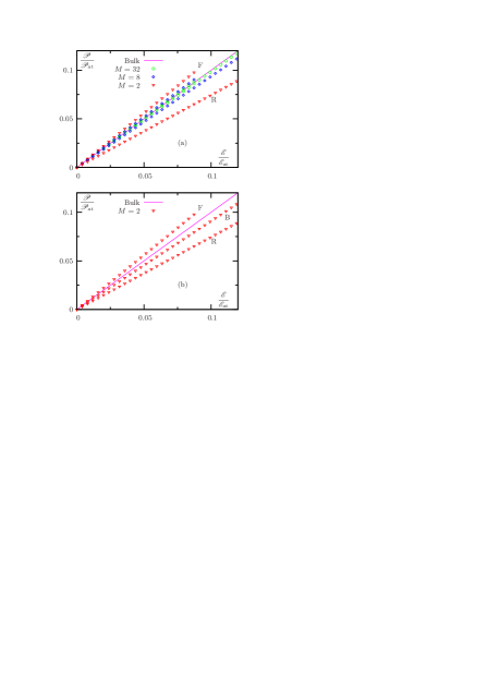
Figure 1: The dipole moment density per unit area, ${\mathscr{P}}$, as a function of the applied field, ${\mathscr{E}}$, for different types of boundary conditions and for films consisting of different numbers of atomic layers, $M$. The continuous line corresponds to the “bulk” (macroscopic) result and the centered symbols represent the results obtained from the DFT. In panel (a), three different values of $M$ are used, as labeled. All data points above the continuous line correspond to F-type boundary conditions and the points below the line correspond to R-type boundary conditions; B-type boundary conditions are not used in this panel. In panel (b), only $M=2$ is used. The two sets of centered symbols below the continuous line in (b) correspond to R- and B-type boundary conditions, as labeled. In both panels, the data points for F-type boundary conditions (above the continuous line) terminate at ${\mathscr{E}}/{\mathscr{E}}_{\rm at}=0.87$; computations for larger values of ${\mathscr{E}}$ (with F-type boundary conditions) are affected by the numerical instability discussed in the text.

In Fig. 1, we plot ${\mathscr{P}}$ as a function of the applied field, ${\mathscr{E}}$, for different widths of the slab and for different types of boundary conditions. In the case of the R- or B-type boundary conditions, the system is stable independent of the strength of the applied field. In the case of F-type boundary condition, we have observed an instability of the charge density for ${\mathscr{E}}\gtrsim 0.1{\mathscr{E}}_{\rm at}$. This instability can be explained by the effect of tunneling, which can result in significant charge accumulation in a biased potential over long periods of time, or after many DFT iterations. The data points affected by this instability are not displayed in Fig. 1. It can be seen that the F-type boundary condition tends to increase ${\mathscr{P}}$ (compared to the macroscopic limit) while the B- or R-type boundary conditions tend to decrease ${\mathscr{P}}$. For all types of boundary conditions, deviations from the macroscopic result are significant when $M=2$ and $M=8$ but small when $M=32$. In the case $M=2$ (Fig. 1b), the B-type curve lies above the R-type curve; a similar result was obtained for other values of $M$ (data not shown). Physically, the behavior illustrated in Fig. 1 can be understood as the result of electron spillover Pustovit and Shahbazyan (2006a, b) (in the case of F-type boundary condition) or as the combined action of the finite charge density of the jellium and of the uncertainty principle (in the case of B- or R-type boundary conditions).

Although the deviation of ${\mathscr{P}}$ from the macroscopic result is obvious in Fig. 1, all curves shown in this figure appear to be linear. To visualize the deviations from linearity, we have computed the nonlinear contribution to the dipole moment density according to

$${\mathscr{P}}_{\rm nonl}={\mathscr{P}}-\frac{h\alpha_{1}}{4\pi}{\mathscr{E}}\ .$$ (54)

The result is plotted in Fig. 2. It can be seen that the correction is negative for R- and B-type boundary conditions. For the F-type boundary condition, the correction is positive and about $200$ times larger in magnitude. An interesting effect can be seen in Fig. 2b. Namely, the B-type boundary condition produces a nonlinear correction of a larger magnitude compared to the R-type boundary condition. This is somewhat unexpected since the data of Fig. 1 suggest that the B-type curve is closer to the macroscopic asymptote. Moreover, we have discovered a non-monotonic dependence of the expansion coefficient $\alpha_{3}$ in (5) on the displacement parameter $\Delta$, as is discussed below.

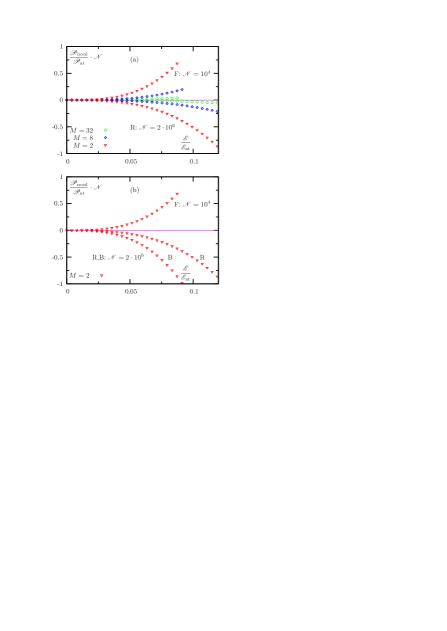
Figure 2: ${\mathscr{P}}_{\rm nonl}$ as a function of the applied field, ${\mathscr{E}}$. The same convention for encoding the different types of boundary conditions and the different numbers of atomic layers as in Fig. 1 is used. Additionally, different numerical normalization factors ${\mathscr{N}}$ have been used for different types of boundary conditions, as labeled.

Recall that the B-type boundary condition involves a displacement of the rigid potential wall from the surface of the metal by the distance $\Delta=\Delta_{\rm B}\approx 0.38\ell$. We can, however, view $\Delta$ as a free parameter. In the case $\Delta=0$, we recover the R-type boundary condition, in the case $\Delta=\infty$ – the F-type boundary condition, and $\Delta=\Delta_{\rm B}$ corresponds to Bardeen’s model. In Fig. 3, we plot the expansion coefficient $\alpha_{3}$ as a function of $\Delta$ for $M=2$. In this figure, we show the data obtained both with and without the exchange-correlation potential. We find that the surprising non-monotonic dependence is observed in both cases. For larger values of $\Delta$, the red curve in Fig. 3 (with exchange-correlation potential included) rapidly grows and saturates at the level of $\alpha_{3}\approx 0.1$ for $\Delta\gtrsim 8\Delta_{\rm B}$ (data not shown). The latter result exactly corresponds to the one obtained with the F-type boundary condition. Note that $\alpha_{1}$ is almost independent of $\Delta$. Qualitatively the same results have been obtained for $M=8$ and $M=32$.

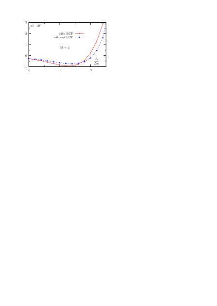
Figure 3: Dependence of $\alpha_{3}$ on $\Delta$ for $M=2$, with and without accounting for the exchange-correlation potential (ECP).

Next, in Fig. 4, we plot ${\mathscr{P}}$ for the B-type boundary condition (with $\Delta=\Delta_{\rm B}$) in a very large interval of ${\mathscr{E}}$, up to ${\mathscr{E}}/{\mathscr{E}}_{\rm at}=10^{3}$. Of course, an applied static electric field of this magnitude is not achievable in practice. However, the situation can be more experimentally favorable in the case of quasistatic fields. Although we do not consider this case directly, it is known that the internal field enhancement factor due to plasmon resonances is of the order of $\omega_{p}/\gamma$, where $\omega_{p}$ is the plasma frequency and $\gamma$ is the Drude relaxation constant. This factor can be as large as $\sim 500$ in the case of silver, and it enters the nonlinear correction to the polarizability in the fourth power Drachev et al. (2004); Govyadinov et al. (2001). Note that the quasistatic approximation (known in the context of DFT as the adiabatic approximation) is applicable as long as $h\omega/c\ll 1$, which easily holds even in the visible spectral range. Also, the electric field intensity in very short laser pulses can be of the order of or higher than the atomic field, and the related physics has attracted considerable recent attention Durach et al. (2010).

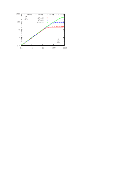
Figure 4: ${\mathscr{P}}$ as a function of the applied field, ${\mathscr{E}}$, for B-type boundary condition and for different numbers of atomic layers, $M$. Centered symbols correspond to DFT results and continuous lines to the analytical expression (55).

In Fig. 4, we also compare the DFT calculations with the expression

$${\mathscr{P}}=\left\{\begin{array}[]{ll}{\displaystyle\frac{h{\mathscr{E}}}{4\pi}}\left[1-{\displaystyle\frac{\ell}{8\pi h}\left|\frac{\mathscr{E}}{\mathscr{E}}_{\rm at}\right|}\right]\ ,&{\rm if}\left|{\displaystyle\frac{\mathscr{E}}{\mathscr{E}}_{\rm at}}\right|\leq{\displaystyle\frac{4\pi h}{\ell}}\ ,\\ {\displaystyle\frac{h^{2}{\mathscr{E}}_{\rm at}}{2\ell}}\ ,&\ \ {\rm otherwise}\ ,\end{array}\right.$$ (55)

which was derived in Ref. Panasyuk et al., 2008 using purely classical arguments. It can be seen that (55) is surprisingly accurate for $M=8$ and especially for $M=32$. This may seem unexpected because (55) contains a nonanalyticity of the form ${\mathscr{E}}|{\mathscr{E}}|$, while the expansion (5) represents a real analytic function. This discrepancy is resolved by noting that (5) has a finite radius of convergence and that an expansion of this type can not, in principle, capture the saturation phenomena illustrated in Fig. 3. On the other hand, numerical DFT calculations can be carried out whether or not (5) converges.

Finally, we investigate the dependence of the coefficients $\alpha_{1}$, $\alpha_{3}$ on the number of atomic layers $M$ for all three types of boundary conditions. The results are shown in Fig. 5. It can be seen that, in all cases, the dependence is monotonic. Comparing the results for R- and B-type boundary conditions, we reconfirm the trend that has been already noted, namely, that B-type boundary conditions produce a smaller finite-size correction to $\alpha_{1}$ (compared to R-type boundary conditions) but a larger nonlinear response.

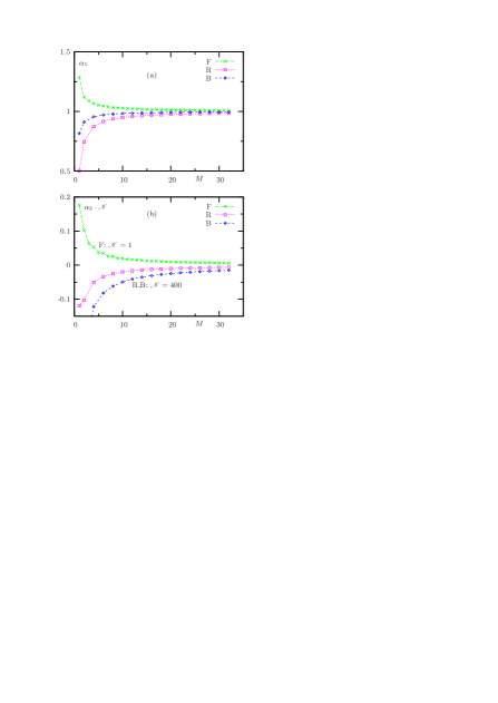
Figure 5: Coefficients $\alpha_{1}$ (a) and $\alpha_{3}$ (b) as functions of the number of atomic layers, $M$, for three different types of boundary conditions. Different numerical normalization factors ${\mathscr{N}}$ have been used for different types of boundary conditions, as labeled.

VI Summary and discussion

We have studied theoretically and numerically polarization of a thin silver film under perpendicularly applied low-frequency external electric field. Three different boundary conditions have been applied at the film surface. It was shown that the sign and magnitude of the nonlinear correction to the film polarizability depends dramatically on the type of boundary condition used. Since all theories involved contain approximations, only comparison with experiment can determine which boundary condition is physically correct.

An obvious shortcoming of the calculations reported herein is that they are carried out for static fields. However, the results can be extended to finite frequencies, as long as relaxation and resonance phenomena are not taken into consideration, that is, if the frequency is far below the lowest plasmon resonance of the system. In practice, this means that the theory can be applied up to THz frequencies. Thus our results are amenable to experimental verification. A possible experimental test could be a measurement of the sign of the real part of the nonlinear susceptibility $\chi^{(3)}$ for a suspension of silver nanodisks at the excitation frequency $\sim 10{\rm GHz}$. The disk thickness should be much smaller than the skin depth, $\delta\approx 0.2\mu{\rm m}$ in this example. Previous experimental measurements of $\chi^{(3)}$ were largely confined to the optical and near-IR spectral regions Uchida et al. (1994); Petrov (1996); Danilova et al. (1996); Torres-Torres et al. (2007), where the sign of ${\rm Re}[\chi^{(3)}]$ can depend on frequency due to the effects of plasmon resonances.

It seems possible to further extend our theory to optical frequencies by utilizing the quasistatic approximation, which is known as the adiabatic approximation in the context of DFT Runge and Gross (1984). In this approximation, all potentials are computed using instantaneous values of the density, for example, by writing for the Hartree interaction potential $U_{\rm H}[\rho_{e}]({\bf r},t)=U_{\rm H}[\rho_{e}({\bf r},t)]$, and similarly for other functionals. This corresponds to neglecting the effects of retardation in the electromagnetic interaction and is adequate as long as $h\omega/c\ll 1$. Note that plasmon resonances and relaxation phenomena can be taken into consideration within quasistatics. However, time-dependent DFT is still relatively unexplored, although some promising results have been obtained Vasiliev et al. (2002).

This work was supported by the NSF under the grant DMR0425780. One of the authors (GYP) is supported by the National Research Council Senior Associateship Award at the Air Force Research Laboratory.

References

• Maier et al. (2003) S. A. Maier, P. G. Kik, H. A. Atwater, S. Meltzer, E. Harel, B. E. Koel, and A. G. Requicha, Nature Materials 2, 229 (2003).
• Prodan et al. (2003) E. Prodan, C. Radloff, N. J. Halas, and P. Nordlander, Science 302, 419 (2003).
• Stockman (2008a) M. I. Stockman, Nature Photonics 2, 327 (2008a).
• Stockman (2008b) M. I. Stockman, New J. Phys. 10, 025031 (2008b).
• Brongersma and Shalaev (2010) M. L. Brongersma and V. M. Shalaev, Science 328, 440 (2010).
• Halas et al. (2011) N. J. Halas, S. Lal, W. S. Chang, S. Link, and P. Nordlander, Chem. Rev. 111, 3913 (2011).
• Dasgupta and Fuchs (1981) B. B. Dasgupta and R. Fuchs, Phys. Rev. B 24, 554 (1981).
• Fuchs and Claro (1987) R. Fuchs and F. Claro, Phys. Rev. B 35, 3722 (1987).
• Ruppin (1992) R. Ruppin, Phys. Rev. B 45, 11209 (1992).
• Panasyuk et al. (2008) G. Y. Panasyuk, J. C. Schotland, and V. A. Markel, Phys. Rev. Lett. 100, 047402 (2008).
• Hache et al. (1986) F. Hache, D. Ricard, and C. Flytzanis, J. Opt. Soc. Am. B 3, 1647 (1986).
• Rautian (1997) S. G. Rautian, Soviet Physics JETP 85, 451 (1997).
• Drachev et al. (2004) V. P. Drachev, A. K. Buin, H. Nakotte, and V. M. Shalaev, Nano Letters 4, 1535 (2004).
• Govyadinov et al. (2001) A. A. Govyadinov, G. Y. Panasyuk, J. C. Schotland, and V. A. Markel, Phys. Rev. B XX, XX (2001).
• Ekardt (1984) W. Ekardt, Phys. Rev. Lett. 52, 1925 (1984).
• Lerme et al. (1999) J. Lerme, B. Palpant, E. Cottancin, M. Pellarin, B. Prevel, J. L. Vialle, and M. Broyer, Phys. Rev. B 60, 16151 (1999).
• Zhu et al. (2008) G. Zhu, M. Mayy, M. Bahoura, B. A. Ritzo, H. V. Gavrilenko, V. I. Gavrilenko, and M. A. Noginov, Opt. Express 16, 15576 (2008).
• Gavrilenko et al. (2010) A. V. Gavrilenko, C. S. McKinney, and V. I. Gavrilenko, Phys. Rev. B 82, 155426 (2010).
• Drachev et al. (2008) V. P. Drachev, U. K. Chettair, A. V. Kildishev, H.-K. Yuan, W. Cai, and V. M. Shalaev, Opt. Express 16, 1186 (2008).
• Qiu et al. (2008) L. Qiu, T. A. Larson, D. Smith, E. Vitkin, M. D. Modell, B. A. Korgel, K. V. Sokolov, E. B. Hanlon, I. Itzkan, and L. T. Perelman, Appl. Phys. Lett. 93, 153106 (2008).
• Shore and Rose (1991) H. B. Shore and J. H. Rose, Phys. Rev. Lett. 66, 2519 (1991).
• Perdew et al. (1990) J. P. Perdew, H. Q. Tran, and E. D. Smith, Phys. Rev. B 42, 11627 (1990).
• Liebsch (1997) A. Liebsch, Electronic Excitations at Metal Surfaces (Plenum Press, 1997), chap. 2.1.3.
• Gunnarsson and Lundqvist (1976) O. Gunnarsson and B. I. Lundqvist, Phys. Rev. B 13, 4274 (1976).
• Bardeen (1936) J. Bardeen, Phys. Rep. 49, 653 (1936).
• Pitarke and Eguiluz (2001) J. M. Pitarke and A. G. Eguiluz, Phys. Rev. B 63, 045116 (2001).
• Han and Liu (2009) Y. Han and D. J. Liu, Phys. Rev. B 80, 155404 (2009).
• Kohn and Sham (1965) W. Kohn and L. J. Sham, Phys. Rep. 140, 1133 (1965).
• Martin (2004) R. M. Martin, Electronic structure: Basic theory and practical methods (Cambridge University Press, 2004).
• Chelvayohan and Mee (1982) M. Chelvayohan and C. H. B. Mee, J. Phys. Chem. 15, 2305 (1982).
• Pustovit and Shahbazyan (2006a) V. N. Pustovit and T. V. Shahbazyan, J. Opt. Soc. Am. A 23, 1369 (2006a).
• Pustovit and Shahbazyan (2006b) V. N. Pustovit and T. V. Shahbazyan, Phys. Rev. B 73, 085408 (2006b).
• Durach et al. (2010) M. Durach, A. Rusina, M. F. Kling, and M. I. Stockman, Phys. Rev. Lett. 105, 086803 (2010).
• Uchida et al. (1994) K. Uchida, S. Kaneko, S. Omi, C. Hata, H. Tanji, Y. Asahara, and A. J. Ikushima, J. Opt. Soc. Am. B 11, 1236 (1994).
• Petrov (1996) D. V. Petrov, J. Opt. Soc. Am. B 13, 1491 (1996).
• Danilova et al. (1996) Y. E. Danilova, S. G. Rautian, and V. P. Safonov, Bulletin of the Russian Acad. Sci. - Physics 60, 374 (1996).
• Torres-Torres et al. (2007) C. Torres-Torres, A. V. Khomenko, J. C. Cheang-Wong, L. Rodriguez-Fernandez, A. Crespo-Sosa, and A. Oliver, Opt. Express 15, 9248 (2007).
• Runge and Gross (1984) E. Runge and E. K. U. Gross, Phys. Rev. Lett. 52, 997 (1984).
• Vasiliev et al. (2002) I. Vasiliev, S. S. Ogut, and J. R. Chelikowsky, Phys. Rev. B 65, 115416 (2002).