Oscillatory dynamos and their induction mechanisms

Abstract

Context. Large-scale magnetic fields resulting from hydromagnetic dynamo action may differ substantially in their time dependence. Cyclic field variations, characteristic for the solar magnetic field, are often explained by an important $\Omega$-effect, i.e. by the stretching of field lines due to strong differential rotation.

Aims. The dynamo mechanism of a convective, oscillatory dynamo model is investigated.

Methods. We solve the MHD-equations for a conducting Boussinesq fluid in a rotating spherical shell. For a resulting oscillatory model, dynamo coefficients have been computed with the help of the so-called test-field method. Subsequently, these coefficients have been used in a mean-field calculation in order to explore the underlying dynamo mechanism.

Results. The oscillatory dynamo model under consideration is of $\alpha^{2}\Omega$-type. Although the rather strong differential rotation present in this model influences the magnetic field, the $\Omega$-effect alone is not responsible for its cyclic time variation. If the $\Omega$-effect is suppressed the resulting $\alpha^{2}$-dynamo remains oscillatory. Surprisingly, the corresponding $\alpha\Omega$-dynamo leads to a non-oscillatory magnetic field.

Conclusions. The assumption of an $\alpha\Omega$-mechanism does not explain the occurrence of magnetic cycles satisfactorily.

1 Introduction

The study of the solar cycle has motivated dynamo theory for many decades. Hence, the solar dynamo has become the prototype of oscillatory dynamos. However, its explanation is still controversial (Jones et al. 2010). Most solar dynamo models have been built on the assumption of an $\alpha\Omega$-dynamo mechanism (Ossendrijver 2003); that is, the poloidal field results from the interaction of helical turbulence with the toroidal field ($\alpha$-effect) whereas the toroidal field is thought to originate from the shearing of poloidal field lines by strong differential rotation ($\Omega$-effect). This attempt is attractive for mainly two reasons:

First, the existence of a strong shear layer at the bottom of the solar convection zone is observationally well established, and the importance of a resulting $\Omega$-effect is non-controversial.

Second, Parker’s plane layer model (Parker 1955) and in particular mean-field electrodynamics (Steenbeck et al. 1966) provide a very elegant theoretical framework for this approach. Within mean-field theory, attention is focused on large scale, i.e. averaged fields, only, and the induction equation may be replaced by a mean-field dynamo equation (Krause & Rädler 1980)

$$\frac{\partial\overline{\@vec{B}}}{\partial t}=\nabla\times(\@vec{\mathcal{E}}+\overline{\@vec{V}}\times\overline{\@vec{B}}-\eta\nabla\times\overline{\@vec{B}})\,,$$ (1)

in which $\overline{\@vec{B}}$ and $\overline{\@vec{V}}$ denote the average magnetic and the average velocity field, $\eta$ stands for the magnetic diffusivity and $\@vec{\mathcal{E}}$ is the mean electromotive force. Moreover, it is assumed that $\@vec{\mathcal{E}}$ is homogeneous in the mean magnetic field and may be replaced by a parameterisation in terms of $\overline{\@vec{B}}$ and its first derivatives

$$\@vec{\mathcal{E}}=\@tens{a}\overline{\@vec{B}}+\@tens{b}\nabla\overline{\@vec{B}}\,.$$ (2)

In (2), the so-called dynamo coefficients $\@tens{a}$ and $\@tens{b}$ are tensors of second and third rank, respectively, and depend only on the velocity field and the magnetic diffusivity. The traditional $\alpha$-effect implemented in a large number of solar dynamo models (e.g. Steenbeck & Krause 1969; Roberts 1972; Roberts & Stix 1972; Stix 1976; Ossendrijver 2003; Brandenburg & Subramanian 2005; Chan et al. 2008) corresponds to the isotropic component of $\@tens{a}$ in relation (2), while the $\Omega$-effect results from the $\phi$-component of the $\nabla\times(\overline{\@vec{V}}\times\overline{\@vec{B}})$ term in equation (1).

However, a strong differential rotation is not a necessary condition for oscillatory solutions of the dynamo equation (1), as has been demonstrated in several papers (see e.g. Rädler & Bräuer 1987; Schubert & Zhang 2000; Rüdiger et al. 2003; Stefani & Gerbeth 2003). These authors construct models in which the toroidal field is likewise generated from the poloidal field by an $\alpha$-effect ($\alpha^{2}$-models) and investigate necessary constraints on $\@tens{a}$, the boundary conditions for the magnetic field and the geometry of the dynamo region in order to obtain oscillatory solutions of (1). Recently, oscillatory dynamo models have also been investigated by means of direct numerical simulations. Mitra et al. (2010) performed dynamo simulations in a wedge-shaped spherical shell with an applied forcing and demonstrate again the existence of oscillatory $\alpha^{2}$-dynamo models.

However, the success of mean-field models in reproducing solar-like variations of the magnetic field relies partly on the large number of free parameters, i.e. on the arbitrary determination of the dynamo coefficients $\@tens{a}$ and $\@tens{b}$. An alternative approach is presented by Pétrélis et al. (2009). They construct amplitude equations guided from symmetry considerations and analyse polarity reversals and oscillatons of the magnetic field resulting from the interaction between two dynamo modes.

Self-consistent, global, convective dynamo models with cyclic magnetic field variations have been bublished by Busse & Simitev (2006), and Goudard & Dormy (2008). Convective dynamo simulations with stress-free mechanical boundary conditions (Busse & Simitev 2006) exhibit a strong and a weak field branch, depending on the initial conditions for the magnetic field. If the magnetic field is initially weak, stress free boundary conditions enable the development of a strong zonal flow carrying most of the kinetic energy and rendering convection ineffective. The magnetic field resulting from these dynamos is rather small scaled, often of quadrupolar symmetry and weak. Oscillatory solutions of the induction equation are typical for this dynamo branch.

A transition from steady to oscillatory dynamos may also be governed by the width of the convection zone; Goudard & Dormy (2008) found oscillatory models by decreasing the shell width. In this study, we follow their approach and analyse the dynamo mechanism for these oscillatory models. In particular, we address the question whether an $\Omega$-effect is responsible for the cyclic variation of the magnetic field. Different from previous work, we determine the dynamo coefficients $\@tens{a}$ and $\@tens{b}$ from direct numerical simulations with the help of the test-field method (Schrinner et al. 2005, 2007). The application of $\@tens{a}$ and $\@tens{b}$ in a mean-field calculation reveals their importance for the generation of the magnetic field.

2 Dynamo calculations

We consider a conducting Boussinesq fluid in a rotating spherical shell and solve the equations of magnetohydrodynamics for the velocity $\@vec{v}$, magnetic field $\@vec{B}$ and temperature $T$ as given by Goudard & Dormy (2008) with the help of the code PaRoDy (Dormy et al. (1998) and further developments),

$$E\left(\frac{\partial\@vec{v}}{\partial t}+\@vec{v}\cdot\nabla\@vec{v}-\nabla^{2}\@vec{v}\right)+2\@vec{z}\times\@vec{v}+\nabla P=$$

$$Ra\frac{\boldsymbol{r}}{r_{o}}T+\frac{1}{Pm}(\nabla\times\@vec{B})\times\@vec{B}\,,$$ (3)

$$\frac{\partial\@vec{B}}{\partial t}=\nabla\times(\@vec{v}\times\@vec{B})+\frac{1}{Pm}\nabla^{2}\@vec{B}\,,$$ (4)

$$\frac{\partial T}{\partial t}+(\@vec{v}\cdot\nabla)(T+T_{s})=\frac{1}{Pr}\nabla^{2}T\,.$$ (5)

Governing parameters are the Ekman number $E=\nu/\Omega L^{2}$, the (modified) Rayleigh number $Ra=\alpha_{T}g_{0}\Delta TL/\nu\Omega$, the Prandtl number $Pr=\nu/\kappa$ and the magnetic Prandtl number $Pm=\nu/\eta$. In these expressions, $\nu$ denotes the kinematic viscosity, $\Omega$ the rotation rate, $L$ the shell width, $\alpha_{T}$ the thermal expansion coefficient, $g_{0}$ is the gravitational acceleration at the outer boundary, $\Delta T$ stands for the temperature difference between the spherical boundaries, $\kappa$ is the thermal and $\eta=1/\mu\sigma$ the magnetic diffusivity with the magnetic permeability $\mu$ and the electrical conductivity $\sigma$. Furthermore, the aspect ratio is defined as the ratio of the inner to the outer shell radius, $r_{i}/r_{o}$; it determines the shell width.

In our models, convection is driven by an imposed temperature gradient between the inner and the outer shell boundary. The mechanical boundary conditions are no slip at the inner and stress free at the outer boundary. Moreover, the magnetic field is assumed to continue as a potential field outside the fluid shell.

Time-averaged dynamo coefficients for an axisymmetric mean magnetic field have been determined from direct numerical simulations as described in detail by Schrinner et al. (2007) and as recently discussed for time-dependent dynamo models by Schrinner (2011). In a second step, these coefficients have been applied in a mean-field model based on equation (1) written as an eigenvalue problem,

$$\sigma\overline{\@vec{B}}=\nabla\times\@tens{D}\overline{\@vec{B}}\,,$$ (6)

in which the linear operator $\@tens{D}$ is defined as

$$\@tens{D}\overline{\@vec{B}}=\overline{\@vec{V}}\times\overline{\@vec{B}}+\@tens{a}\overline{\@vec{B}}+\@tens{b}\nabla\overline{\@vec{B}}-\frac{1}{Pm}\nabla\times\overline{\@vec{B}}\,.$$ (7)

The time evolution of each mode is determined by its eigenvalue $\sigma$ and proportional to $\exp{(\sigma t)}$. For more details concerning the eigenvalue calculation, we refer to Schrinner et al. (2010b).

We also consider the evolution of a kinematically advanced magnetic field, $\@vec{B}_{\mathrm{Tr}}$, governed by a second induction equation

$$\frac{\partial\@vec{B}_{\mathrm{Tr}}}{\partial t}=\nabla\times(\@vec{v}\times\@vec{B}_{\mathrm{Tr}})+\frac{1}{Pm}\nabla^{2}\@vec{B}_{\mathrm{Tr}}\,.$$ (8)

The tracer field $\@vec{B}_{\mathrm{Tr}}$ experiences the self-consistent velocity field at each time step but does not contribute to the Lorentz force and is passive in this sense (see also Schrinner et al. 2010a). Its evolution will be compared with mean-field results originating likewise from a kinematic approach. Moreover, a kinematically advanced tracer field allows us to test for the influence of the $\Omega-$effect in direct numerical simulations. In a numerical experiment, we subtract the contribution of the $\Omega-$effect and the mean meridional flow in the equation for the tracer field,

$$\frac{\partial\@vec{B}_{\mathrm{Tr}}}{\partial t}=\nabla\times(\@vec{v}\times\@vec{B}_{\mathrm{Tr}})+\frac{1}{Pm}\nabla^{2}\@vec{B}_{\mathrm{Tr}}-\nabla\times(\overline{\@vec{V}}\times\overline{\@vec{B}}_{\mathrm{Tr}})\,,$$ (9)

and study in this way the outcome of a kinematic $\alpha^{2}$-dynamo.

3 Results

The model under consideration has been previously studied by Goudard & Dormy (2008). It is defined by $E=10^{-3}$, $Ra=100\,(=2.8\,Ra_{c})$, $Pm=5$, $Pr=1$ and an aspect ratio of $0.65$. Except for the stress-free mechanical boundary condition applied at $r=r_{o}$ and an increased aspect ratio, the governing parameters are those of a rather simple, quasi-steady benchmark dynamo (Christensen et al. 2001). However, Goudard & Dormy (2008) report a transition from steady, dipolar to oscillatory models for these parameter values. Note that the model requires a rather high angular resolution up to harmonic degree $l_{\mathrm{max}}=112$.

Figure 1 displays the radial component of the velocity field at a given radial level. A typical columnar convection pattern is visible, even though the convection columns are noticeably disturbed by the influence of the curved boundaries and a strong zonal flow carrying about 50 per cent of the kinetic energy. The magnetic Reynolds number based on the rms-velocity and the shell width, $Rm=v_{\mathrm{rms}}\,L/\eta$, is about 90. The flow is symmetric with respect to the equatorial plane and convection takes place only outside the inner core tangent cylinder.

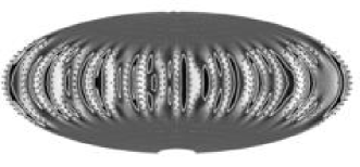
Figure 1: Snapshot of the radial velocity of the considered dynamo model at $r=0.79\,r_{o}$. The velocity component has been normalised by its maximum absolute value, $\@vec{v}_{r,\,\mathrm{max}}=24.46\,\nu/L$. Hence, the colour coding ranges from $-1$, white, to $+1$, black. Contour lines correspond to $\pm 0.2$ and $\pm 0.6$.

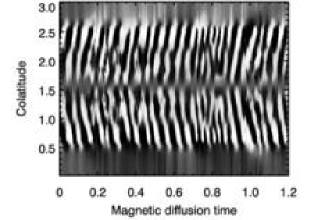
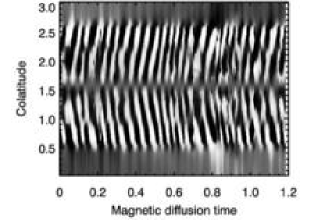
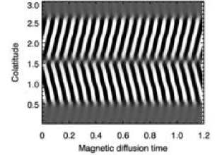
Figure 2: Azimuthally averaged radial magnetic field at the outer shell boundary varying with time (butterfly diagram) resulting from a self-consistent calculation (top), kinematic calculation according to (8) (middle) and mean-field calculation (bottom). The contour plots have been normalised by their maximum absolute value at each time step considered. The colour coding ranges from $-1$, white, to $+1$, black.

The evolution of the magnetic field is cyclic. In figure 2 (top), contours of the azimuthally averaged radial magnetic field at the outer shell boundary varying with time are plotted in a so-called butterfly diagram. A dynamo wave migrates away from the equator until it reaches mid-latitudes where the inner core tangent cylinder intersects the outer shell boundary. The magnetic field looks rather small scaled and multipolar. This is confirmed by the magnetic energy spectrum which is essentially white, except for a negligible dipole contribution. Furthermore, the magnetic field is weak, as expressed by an Elsasser number of $\Lambda=B^{2}_{\mathrm{rms}}/(\mu\rho\eta\Omega)=0.13$.

The kinematically advanced tracer field grows slowly in time, i.e. the model under consideration is kinematically unstable according to the classification by Schrinner et al. (2010a). But, deviations of the tracer field from the actual field are hardly noticeable in the field morphology. Moreover, the very same dynamo wave persists in the kinematic calculation (see also Goudard & Dormy (2008)), as visible in figure 2 (middle). Note that the tracer field in figure 2 has evolved from random initial conditions.

A mean-field calculation based on the dynamo coefficients $\@tens{a},\,\@tens{b}$ and the mean flow $\overline{\@vec{V}}$ determined from the self-consistent model is presented in the bottom line of figure 2. The fastest growing eigenmodes form a conjugate complex pair and give rise to a dynamo wave which compares nicely with the direct numerical simulations. Since this model depends on the full $\@tens{a}$-tensor and the mean flow, we refer to it as an $\alpha^{2}\Omega$-dynamo.

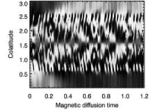
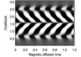
Figure 3: Azimuthally averaged radial magnetic field at the outer shell boundary varying with time (butterfly diagram) resulting from a kinematic calculation with subtracted $\Omega$-effect (top) and a corresponding mean-field calculation (bottom). The contour plots are presented as in figure (2).

The influence of the differential rotation may be suppressed in the kinematic calculation of the tracer field without changing any other component of the flow. A butterfly diagram resulting from a kinematically advanced field according to equation (9) is presented in figure 3 (top). The evolution of the magnetic field is again cyclic. Apart from small-scale variations on shorter time scales, a dynamo wave migrates from mid-latitudes towards the equator. This is in agreement with a corresponding mean-field calculation in which the mean flow $\overline{\@vec{V}}$ in (7) has been canceled: The bottom chart of figure 3 provides the butterfly diagram stemming from the fastest growing eigenmodes of the resulting $\alpha^{2}$-dynamo. An explanation why direct numerical simulations and mean field calculations compare somewhat better in figure 2 than in figure 3 is provided in appendix A.

The time evolution of the related $\alpha\Omega$-dynamo is of further interest. As the $\alpha$-effect is not directly accessible in direct numerical simulations, the corresponding $\alpha\Omega$-dynamo can be realised in a mean-field calculation, only. In a first attempt, we have set $\@tens{a}_{rr}=\@tens{a}_{\theta\theta}=0$ in order to suppress the generation of toroidal field from poloidal field by an $\alpha$-effect. Both components make major contributions to this process. The leading eigenmode resulting from this calculation is shown in figure 4; it is real, i.e. non-oscillatory, and close to marginal stability. The results remain similar if we neglect further, non-diagonal components of $\@tens{a}$.

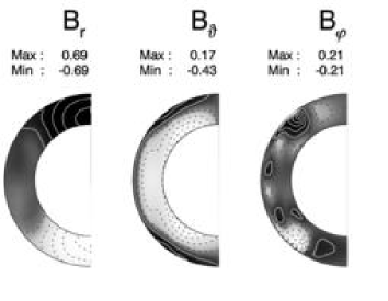
Figure 4: The leading dipolar eigenmode resulting from a mean-field calculation with $a_{rr}=a_{\theta\theta}=0$. Contour plots of all three components are presented, each normalised separately by their maximum absolute values. Maxima and minima are written next to each plot. The colour coding ranges from $-1$, white, to $+1$, black, and contour lines correspond to $\pm 0.1$, $\pm 0.3$, $\pm 0.5$, $\pm 0.7$ and $\pm 0.9$.

4 Discussion

The Frequency and the propagation direction of the dynamo wave visible in figure 2 depend strongly on the differential rotation, in agreement with Busse & Simitev (2006). We follow their approach and give an estimate for the cycle frequency applying Parker’s plane layer formalism (Parker 1955). To this end, we introduce a Cartesian coordinate system $(x,y,z)$ corresponding to the $(\phi,\theta,r)$ directions and define mean quantities to be x-independent. Moreover, we write $\overline{\@vec{B}}=B\@vec{e_{x}}+\@vec{B_{p}}=B\@vec{e_{x}}+\nabla\times A\@vec{e_{x}}$ and reformulate (1) in the following simplified manner

$$\frac{\partial A}{\partial t} = \@tens{\alpha}_{xx}B+\frac{1}{Pm}\nabla^{2}A\,,$$ (10)

$$\frac{\partial B}{\partial t} = -\frac{\partial}{\partial y}(\@tens{\alpha}_{zz}\frac{\partial A}{\partial y})+\frac{\mathrm{d}\overline{\@vec{V}}_{x}}{\mathrm{d}z}\frac{\partial A}{\partial y}+\frac{1}{Pm}\nabla^{2}B\,.$$ (11)

In the above equations, we have considered only the dominant diagonal components of $\@tens{a}$, $\@tens{a}_{rr}$ and $\@tens{a}_{\phi\phi}$ corresponding to $\@tens{\alpha}_{zz}$ and $\@tens{\alpha}_{xx}$; all components of $\@tens{b}$ and the mean meridional flow have been neglected. Furthermore, $\overline{\@vec{V}}$ has been assumed to depend only on $z$. Then, the ansatz

$$(A,B)=(\hat{A},\hat{B})\exp(i\@vec{k}\cdot\@vec{x}+\sigma t)\,,$$ (12)

leads to

$$p\hat{A} = \alpha_{xx}\hat{B}\,,$$ (13)

$$p\hat{B} = \left(\alpha_{zz}k_{y}^{2}+ik_{y}\left(\frac{\mathrm{d}\overline{\@vec{V}}}{\mathrm{d}z}-\frac{\partial\alpha_{zz}}{\partial y}\right)\right)\hat{A}\,,$$ (14)

with $p=\sigma+|\@vec{k}|^{2}/Pm$. From (13), (14), we derive a dispersion relation

$$p^{2}=\alpha_{xx}\left(\alpha_{zz}k_{y}^{2}+ik_{y}\left(\frac{\mathrm{d}\overline{\@vec{V}}}{\mathrm{d}z}-\frac{\partial\alpha_{zz}}{\partial y}\right)\right)\,,$$ (15)

from which the real and the imaginary part of $\sigma$ can be calculated. If $\alpha_{xx}$ is positive (e.g. in the northern hemisphere), it follows

$$\lambda = \Re(\sigma)=-|\@vec{k}|^{2}/Pm$$ (16)

$$+\sqrt{\frac{\alpha_{xx}}{2}}\left(\sqrt{(\alpha_{zz}k_{y}^{2})^{2}+\left(\frac{\mathrm{d}\overline{\@vec{V}}}{\mathrm{d}z}-\frac{\partial\alpha_{zz}}{\partial y}\right)^{2}k_{y}^{2}}+\alpha_{zz}k_{y}^{2}\right)^{1/2}\,$$

and

$$\omega = \Im(\sigma)=$$ (17)

$$\pm\sqrt{\frac{\alpha_{xx}}{2}}\left(\sqrt{(\alpha_{zz}k_{y}^{2})^{2}+\left(\frac{\mathrm{d}\overline{\@vec{V}}}{\mathrm{d}z}-\frac{\partial\alpha_{zz}}{\partial y}\right)^{2}k_{y}^{2}}-\alpha_{zz}k_{y}^{2}\right)^{1/2}\,.$$

The sign in (17) is determined by the sign of $k_{y}(\mathrm{d}\overline{\@vec{V}}/\mathrm{d}z-\partial\alpha_{zz}/\partial y)$. If we further assume that the frequency is dominated by differential rotation and neglect the $\alpha$-terms in (17), we estimate similar to Busse & Simitev (2006)

$$\omega=\Im(\sigma)\approx\pm\left(\frac{\pi}{L^{2}}\@tens{\alpha}_{xx}\sqrt{2\overline{E}_{T}}\right)^{1/2}\,.$$ (18)

In (18), $\overline{E}_{T}$ denotes the the kinetic energy density due to the axisymmetric toroidal velocity field and $k_{y}\approx 2\pi/L$ has been used. Approximating $\@tens{\alpha}_{xx}$ by the rms-value of $\@tens{a}_{\phi\phi}$, $\@tens{\alpha}_{xx}=11.50\,\nu/L$, and with $E_{T}=71\,\nu^{2}/L^{2}$, we find $\omega\approx\pm 103.7\,\eta/L^{2}$ which is surprisingly close to $\omega=\pm 100.95\eta/L^{2}$ in the full calculation presented in figure 2. Note that $\@tens{\alpha}_{xx}$ and $\mathrm{d}\overline{\@vec{V}}/\mathrm{d}z$ are of the same order of magnitude and contribute equally to $\omega$. The sign in (18) is determined by the sign of the product $\@tens{a}_{\phi\phi}\,\partial\overline{\@vec{V}}_{\phi}/\partial r$ which is positive in the northern and negative in the southern hemisphere. Therefore, our estimate in (18) predicts a dynamo wave migrating away from the equator. This is in agreement with the simulations shown in figure 2.

However, the attempt to describe the model under consideration as an $\alpha\Omega$-dynamo fails. An oscillatory mode with a frequency close to the above estimate turns out to be clearly subcritical in a mean-field calcuation, if $\@tens{a}_{rr}$ and $\@tens{a}_{\theta\theta}$ are omitted. Instead, this model is governed by a real, dipolar mode close to marginal stability (see figure 4). Hence, the $\Omega$-effect is only partly responsible for the generation of the mean azimuthal field, as confirmed by figure 5. The chart in the middle compares the $\Omega$-effect, $r\overline{\@vec{B}}_{r}\,\partial(r^{-1}\overline{\@vec{V}}_{\phi})/\partial r+r^{-1}\sin\theta\,\overline{\@vec{B}}_{\theta}\,\partial(\sin\theta^{-1}\overline{\@vec{V}}_{\phi})/\partial\theta$ in greyscale with the mean azimuthal field displayed by superimposed contour lines. In particular, the elongated flux patches close to the inner core tangent cylinder are, if at all, negatively correlated with the $\Omega$-effect. Consistent with this finding, the poloidal axisymmetric magnetic energy density exceeds the toroidal one by 20%.

Differential rotation alone is not responsible for the cyclic time evolution of the magnetic field, despite its influence on the frequency and the propagation direction of the dynamo wave. This is most clearly visible in figure 3. Simulations without differential rotation still lead to a dynamo wave even though its frequency and propagation direction have changed. In the framework of Parker’s plane layer formalism, the frequency of this oscillatory $\alpha^{2}$-dynamo depends crucially on $-\partial\@tens{\alpha}_{zz}/\partial y$ instead of $d\overline{\@vec{V}}_{x}/dz$. Note the additional minus sign, which might explain the reversed propagation direction if the assume that $\partial\alpha_{zz}/\partial y$ is predominantly positive. But different from the radial derivative of the mean azimuthal flow, $(1/r)\,\partial\@tens{a}_{rr}/\partial\theta$ is highly structured, changes sign in radial direction and exhibits localised patches of low negative values (see figure 5). Therefore, we do not attempt to give an estimate for the frequency similar to (18).

In order to better understand the influence of the mean flow on the frequency of the dynamo wave, we have gradually changed the amplitude of $\overline{\@vec{V}}$ in a series of kinematic calculations. Results are presented in figure 6. Stars denote frequencies obtained from eigenvalue calculations according to (6), wheras triangles stand for frequencies estimated from kinematic results due to equation (8). In both cases, the amplitude of the mean flow $\overline{\@vec{V}}$ has been varied by multiplication with a scale factor $f$. For $f=1$, the original calculation is retained, while for $f=0$, we reproduce the $\alpha^{2}$-dynamo already discussed above. Frequencies of dynamo waves resulting from direct numerical simulations according to (8) have been meassured for $f=1,\,0.7$, and $0.5$. Owing to the turbulence present in the simulations, these are rather rough estimates and error bars have been included. Nevertheless, the results obtained are in satisfactory agreement with the eigenvalue calculations. The frequencies in figure 6 decrease continously with decreasing scale factors. If the amplitude of $\overline{\@vec{V}}$ is reduced to 25 per cent of its original value, $\omega$ changes sign and the propagation direction of the dynamo wave is reversed. The dashed-dotted line in figure 6 gives $\omega$ according to (18) as predicted for an $\alpha\omega$-dynamo. It matches the numerical results if $\mathrm{d}\overline{\@vec{V}}/\mathrm{d}z$ dominates in (17) but deviates clearly for smaller amplitudes. On the other hand, it is illustrative to use relation (17) to model the dependence of $\omega$ on the mean flow. If we set $\partial\alpha_{zz}/dy=0.25\,\mathrm{d}\overline{\@vec{V}}/\mathrm{d}z$ and determine a representative value for $\alpha_{zz}$ inverting (17) for $\mathrm{d}\overline{\@vec{V}}/\mathrm{d}z=0$ and $\omega=-29.15\eta/L^{2}$, the dashed line in figure 6 results from (17). It fits the numerical data rather well and converges towards the frequencies predicted for an $\alpha\omega$-dynamo, if the amplitude of $\overline{\@vec{V}}$ is sufficiently high.

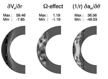
Figure 5: Left: $\partial\overline{\@vec{V}}_{\phi}/\partial r$ in units of $\nu/L^{2}$. Middle: $\Omega$-effect as given by $r\overline{\@vec{B}}_{r}\,\partial(r^{-1}\overline{\@vec{V}}_{\phi})/\partial r+r^{-1}\sin\theta\,\overline{\@vec{B}}_{\theta}\,\partial(\sin\theta^{-1}\overline{\@vec{V}}_{\phi})/\partial\theta$ (greyscale) and $\overline{\@vec{B}}_{\phi}$ (superimposed contour lines, solid [dashed] lines indicate positive [negative] values). Right: $(1/r)\,\partial\@tens{a}_{rr}/\partial\theta$ in units of $\nu/L^{2}$. The contour plots are presented in the same style as in figure 4.

Let us stress again that some caution is needed in applying the present mean-field analysis to non-linear direct numerical simulations, as the the dynamo model considered here is kinematically unstable. Strictly speaking, our mean-field results are only relevant for the kinematically advanced tracer field. But, because the model is close to dynamo onset and only weakly non-linear, we believe that our interpretation is also valid for the fully self-consistent field. This is in particular confirmed by the rather good agreement of the three butterfly diagrams presented in figure 2.

Figure 6: Frequencies resulting from kinematic calculations in which the amplitude of the mean flow has been changed by multiplication with a scale factor, $f$. Stars denote frequencies stemming from an eigenvalue calculation according to (6), whereas triangles are estimates obtained from kinematic results due to (8). The dashed-dotted line gives frequencies as predicted for an $\alpha\omega$-dynamo by (18), while the dashed line represents $\omega$ as a function of $\overline{\@vec{V}}$ for an $\alpha^{2}\omega$-dynamo according to (17).

5 Conclusions

A particular dynamo mechanism does not seem to be responsible for the occurrence of periodically time-dependent magnetic fields. It turns out, that the influence of the large-scale radial shear (the $\Omega$-effect), is not necessary for cyclic field variations. Instead, the action of small-scale convection, represented by a spatially structured dynamo coefficient $\@tens{a}_{rr}$, happens to be essential. For the model presented here, small convective length scales are forced by a thin convection zone. Further investigations are needed to assess whether our finding is representative for a wider class of oscillatory models.

Appendix A The use of time averaged dynamo coefficients

In the following, azimuthal averages are, as throughout in the paper, denoted by an overbar, time averages are expressed by brackets, $<\cdots>$. Initially, dynamo coefficients have been determined for an azimuthally averaged, mean magnetic field $\overline{\@vec{B}}$. Hence, the evolution of the latter is given by

$$\frac{\partial\overline{\@vec{B}}}{\partial t}=\nabla\times(\@tens{a}\overline{\@vec{B}}+\@tens{b}\nabla\overline{\@vec{B}}+\overline{\@vec{V}}\times\overline{\@vec{B}}-\frac{1}{Pm}\nabla\times\overline{\@vec{B}})\,.$$ (19)

But, the dynamo coefficients $\@tens{a}$, $\@tens{b}$ and the mean flow $\overline{\@vec{V}}$ vary stochastically in time. In order to describe the average dynamo action, we take in addition the time average of these quantities and write approximatively,

$$\frac{\partial\overline{\@vec{B}}}{\partial t}\approx\nabla\times(<\!\@tens{a}\!>\overline{\@vec{B}}+<\!\@tens{b}\!>\nabla\overline{\@vec{B}}+<\!\overline{\@vec{V}}\!>\times\overline{\@vec{B}}-\frac{1}{Pm}\nabla\times\overline{\@vec{B}}).$$ (20)

We emphasise that there is no a priori relation between the left hand side and the right hand side of equation (20). The actual, azimuthally averaged magnetic field will deviate from our mean-field description the stronger, the more $\@tens{a}$, $\@tens{b}$ and $\overline{\@vec{V}}$ fluctuate in time. Among these three quantities, the mean flow $\overline{\@vec{V}}$ is almost time independent, whereas $\@tens{a}$ and $\@tens{b}$ vary considerably. This is the reason, why the butterfly diagrams in figure 2 are in better agreement than in figure 3, for which the stabilizing influence of the mean flow has been omitted.

References

- Brandenburg & Subramanian (2005) Brandenburg, A. & Subramanian, K. 2005, Phys. Rep, 417, 1
- Busse & Simitev (2006) Busse, F. H. & Simitev, R. D. 2006, Geophys. Astrophys. Fluid Dyn., 100, 341
- Chan et al. (2008) Chan, K. H., Liao, X., & Zhang, K. 2008, ApJ, 682, 1392
- Christensen et al. (2001) Christensen, U. R., Aubert, J., Cardin, P., et al. 2001, Phys. Earth Planet. Inter., 128, 25
- Dormy et al. (1998) Dormy, E., Cardin, P., & Jault, D. 1998, Earth Planet. Sci. Lett., 160, 15
- Goudard & Dormy (2008) Goudard, L. & Dormy, E. 2008, Europhys. Lett., 83, 59001
- Jones et al. (2010) Jones, C. A., Thompson, M. J., & Tobias, S. M. 2010, Space Sci. Rev., 152, 591
- Krause & Rädler (1980) Krause, F. & Rädler, K. 1980, Mean-field magnetohydrodynamics and dynamo theory, ed. Goodman, L. J. & Love, R. N. (Oxford, Pergamon Press, Ltd., 1980. 271 p.)
- Mitra et al. (2010) Mitra, D., Tavakol, R., Käpylä, P. J., & Brandenburg, A. 2010, ApJ, 719, L1
- Ossendrijver (2003) Ossendrijver, M. 2003, A&A Rev., 11, 287
- Parker (1955) Parker, E. N. 1955, ApJ, 122, 293
- Pétrélis et al. (2009) Pétrélis, F., Fauve, S., Dormy, E., & Valet, J. 2009, Phys. Rev. Lett., 102, 144503
- Rädler & Bräuer (1987) Rädler, K. & Bräuer, H. 1987, Astron. Nachr., 308, 101
- Roberts (1972) Roberts, P. H. 1972, Phil. Trans. R Soc. Lond. A, 272, 663
- Roberts & Stix (1972) Roberts, P. H. & Stix, M. 1972, A&A, 18, 453
- Rüdiger et al. (2003) Rüdiger, G., Elstner, D., & Ossendrijver, M. 2003, A&A, 406, 15
- Schrinner (2011) Schrinner, M. 2011, in preparation
- Schrinner et al. (2005) Schrinner, M., Rädler, K., Schmitt, D., Rheinhardt, M., & Christensen, U. 2005, Astron. Nachr., 326, 245
- Schrinner et al. (2007) Schrinner, M., Rädler, K., Schmitt, D., Rheinhardt, M., & Christensen, U. R. 2007, Geophys. Astrophys. Fluid Dyn., 101, 81
- Schrinner et al. (2010a) Schrinner, M., Schmitt, D., Cameron, R., & Hoyng, P. 2010a, Geophys. J. Int., 182, 675
- Schrinner et al. (2010b) Schrinner, M., Schmitt, D., Jiang, J., & Hoyng, P. 2010b, A&A, 519, A80+
- Schubert & Zhang (2000) Schubert, G. & Zhang, K. 2000, ApJ, 532, L149
- Steenbeck & Krause (1969) Steenbeck, M. & Krause, F. 1969, Astron. Nachr., 291, 49
- Steenbeck et al. (1966) Steenbeck, M., Krause, F., & Rädler, K. 1966, Zeit. Nat. A, 21, 369
- Stefani & Gerbeth (2003) Stefani, F. & Gerbeth, G. 2003, Phys. Rev. E, 67, 027302
- Stix (1976) Stix, M. 1976, A&A, 47, 243