Subdiffusive dynamics in washboard potentials: two different approaches
and different universality classes

Abstract

We consider and compare two different approaches to the fractional subdiffusion and transport in washboard potentials. One is based on the concept of random fractal time and is associated with the fractional Fokker-Planck equation. Another approach is based on the fractional generalized Langevin dynamics and is associated with anti-persistent fractional Brownian motion and its generalizations. Profound differences between these two different approaches sharing the common adjective “fractional” are explained in spite of some similarities they share in the absence of a nonlinear force. In particular, we show that the asymptotic dynamics in tilted washboard potentials obey two different universality classes independently of the form of potential.

I Introduction

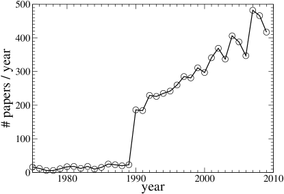
Figure 1: Number of papers on the subject “anomalous diffusion” published per year according to the ISI Web of Science, Thomson-Reuters. Notice the “phase transition”-like rise during 1990.

Anomalous diffusion becomes an increasingly popular subject with the number of papers published per year growing fast over last twenty years after a distinct rise occurred in 1990 (cf. Fig. 1). Since then, it spreads from such typical physical applications as charge transport in disordered solids and hot plasmas to biophysical applications and even quantitative finance Shlesinger1 ; Scher ; Bouchaud ; Hughes ; Shlesinger ; Metzler ; West ; West2 ; Zaslavsky ; Saxton ; Seisenberg ; Tolic ; GH04 ; Golding ; Wilhelm ; Amblard ; Szymanski ; Kou ; Mizuno ; Reuveni .

There are several sufficiently generic physical mechanisms and accompanying theoretical approaches to describe the complexity of anomalous transport processes. One approach is intrinsically based on the physical picture of a stochastic time clock Shlesinger1 ; Scher ; Hughes ; Shlesinger ; Metzler ; Sokolov1 . It models random sojourns of a travelling particle in trapping domains of a disordered solid, e.g. due to energy disorder. After a random time spent in some spatially located trapping domain the particle jumps to a neighboring domain, or maybe farther, and such a jumping process continues in time. The jump directions and their lengths are not correlated from jump to jump and the next clock period is not correlated with those passed (semi-Markovian assumption ). Such a random clock is completely characterized by the probability density of clock periods $\psi(\tau)$. In a given time interval $t$ there will be a random number of jumps $n$, or stochastic clock periods completed. However, if the mean clock period $\langle\tau\rangle$ exists, the probability distribution $p(n,t)$ of “ticking” $n$ times within the observer time window $t$ becomes for large $n$ a very sharp function Hughes around $n^{*}(t)=t/\langle\tau\rangle$, as characterized by the relative dispersion, $\langle\delta n^{2}(t)\rangle^{1/2}/\langle n(t)\rangle$ (see Appendix A). In the continuum medium approximation the trapping domains shrink to points. Then, $\langle\tau\rangle$ can be made arbitrarily small and $n$ becomes quasi-continuous variable for a finite $t$. Correspondingly, the probability density of intrinsic time, $\tau(t)=n(t)\tau_{\rm sc}$, where $\tau_{\rm sc}$ is a time-scaling parameter, an intrinsic clock time unit equal to the duration of time period for the regular clock, assumes a delta-function, $p(\tau)=\delta(\tau-t)$, and the stochastic clock is not different from the regular one.

The situation changes dramatically if the mean of sojourns does not exist, or better to say, it exceeds largely a typical time required to diffuse across the physical medium of a finite size. Then, $p(n,t)$ is not a sharp function around the mean number $\langle n(t)\rangle$. This is the case, for example, when $\psi(\tau)$ possesses a long tail, $\psi(\tau)\propto(\tau/\tau_{\rm sc})^{-1-\alpha}$ for $\tau/\tau_{\rm sc}\to\infty$ with $0<\alpha<1$. This implies a divergent mean $\langle\tau\rangle\to\infty$, and diverging higher moments as well. Nevertheless, $\langle n(t)\rangle\propto(t/\tau_{\rm sc})^{\alpha}$ exists for any finite $t$ and it scales sublinearly with the physical time $t$ (see in Appendix A). In terms of the one-sided Levy distribution density ${\cal L}_{\alpha}(z)$, $p(n,t)=(t/\tau_{\rm sc}){\cal L}_{\alpha}(n^{-1/\alpha}t/\tau_{\rm sc})/(\alpha n^{1/\alpha+1})$.

Consider now an ensemble of particles. Until time $t$, each particle has accomplished an individual number of intrinsic time periods corresponding to the intrinsic time $\tau(t)$ which becomes a random variable broadly distributed: all the particles have their own history, maintaining individuality and avoiding the fate of self-averaging even in the strict limit $t\to\infty$. Only an additional ensemble averaging smears out this principal randomnessSokolov1 ; He ; Lubelski . The unbiased diffusion becomes anomalously slow and nonergodic with the spatial variance of a cloud of particles growing sublinearly, $\langle\delta x^{2}(t)\rangle\propto\langle n(t)\rangle\propto t^{\alpha}$. Such a nonergodic approach to subdiffusion seems appropriate for disordered solids, e.g. thin amorphous films Scher ; Hughes , with a more recent example provided by ${\rm TiO_{2}}$ nanocrystalline electrodes in the Grätzel’s photovoltaic cell elements Nelson . For charged carriers within such media one can create a potential energy profile $U(x)$ by applying an electrical field of spatially distributed fixed charges and a static external electrical field. Then in the continuum approximation subdiffusion can be described by the fractional Fokker-Planck equation (FFPE) Metzler ; Metzler99 ; Barkai01

$$\frac{\partial}{\partial t}P(x,t)=\sideset{{}_{0}}{{}_{t}}{\mathop{\hat{D}}^{1-\alpha}}\left[-\frac{\partial}{\partial x}\frac{f(x)}{\eta_{\alpha}}+\kappa_{\alpha}\frac{\partial^{2}}{\partial x^{2}}\right]P(x,t)\,,$$ (1)

where $f(x)=-dU(x)/dx$ is the force, $\eta_{\alpha}$ is the fractional friction coefficient related to the fractional subdiffusion coefficient $\kappa_{\alpha}$ by the generalized Einstein relation, $\eta_{\alpha}=k_{B}T/\kappa_{\alpha}$, at temperature $T$ and

$$\sideset{{}_{t_{0}}}{{}_{t}}{\mathop{\hat{D}}^{\gamma}}P(x,t)=\frac{1}{\Gamma(1-\gamma)}\frac{\partial}{\partial t}\int_{t_{0}}^{t}\mathrm{d}t^{\prime}\,\frac{P(x,t^{\prime})}{(t-t^{\prime})^{\gamma}}\,,$$ (2)

is the Riemann-Liouville operator of the fractional derivative Mainardi , where $0<\gamma<1$ and $\Gamma(x)$ is the gamma-function. The FFPE (1) can be derived within the above continuous time random walk (CTRW) framework. It can also be written in the form using the Caputo fractional derivative Mainardi

$$\sideset{{}_{t_{0}}}{{}_{*}}{\mathop{D}^{\gamma}}P(x,t):=\frac{1}{\Gamma(1-\gamma)}\int_{t_{0}}^{t}dt^{\prime}\frac{\partial P(x,t^{\prime})/\partial t^{\prime}}{(t-t^{\prime})^{\gamma}}$$ (3)

acting on the left hand side, yielding GH06

$$\sideset{{}_{0}}{{}_{*}}{\mathop{D}^{\alpha}}P(x,t)=\kappa_{\alpha}\frac{\partial}{\partial x}\left(e^{-\beta U(x)}\frac{\partial}{\partial x}\,e^{\beta U(x)}P(x,t)\right)=-\frac{\partial J(x,t)}{\partial x}\,,$$ (4)

in the transport form. Here, $\beta=1/(k_{B}T)$ is inverse temperature and

$$J(x,t)=-\kappa_{\alpha}e^{-\beta U(x)}\frac{\partial}{\partial x}\,e^{\beta U(x)}P(x,t)$$ (5)

is the subdiffusive flux. It should be emphasized that a non-Markovian Fokker-Planck equation never defines the corresponding non-Markovian process completely HT77 ; Grabert . It allows to find merely the single-time, conditional, and double-time probability densities, but never the multi-time probability densities. However, the FFPE dynamics can be nicely simulated from the underlying CTRW with the nearest neighbors jumps only GH06 ; H06 .

A quite different approach to subdiffusion is associated with the fractional Brownian motion Mandelbrot . Here, the principal issue is the long-range anticorrelations in the particle displacements, positive increments follow with a greater probability by negative increments and vice versaGoychuk09 ; Jeon , which can reflect e.g. the phenomenon of viscoelasticity in complex glass-forming liquids above, but close to the glass transition. The Brownian particle is temporally trapped in a trap (cage effect) by an elastic force with spring constant $G(t)$ which decays to zero in time releasing the particle. Let’s assume that the motion starts at $t_{0}$, $v(t)=\dot{x}(t)=0$ for $t<t_{0}$. In the linear approximation, on the particle acts a viscoelastic force $F_{\rm v-el}(t)=-\int_{t_{0}}^{t}G(t-t^{\prime})\dot{x}(t^{\prime})dt^{\prime}$, where $\dot{x}(t)$ is the particle’s instant velocity. The first theory of viscoelasticity has been proposed by J. Clerk Maxwell Maxwell in 1867. It corresponds to $G(t)$ exponentially decaying in time, $G(t)=G_{0}\exp(-t/\tau_{0})$, with a relaxation time constant $\tau_{0}$. Departing from the phenomenon of elasticity in solids Maxwell derived the phenomenon of viscosity in liquids in the limit where the decay of elastic modulus is very fast on the time scale of $v(t)$ change, which corresponds to $G(t)=2\eta_{0}\delta(t)$, with $\eta_{0}=G_{0}\tau_{0}$ being the viscous friction coefficient. In the theory of generalized Brownian motion, $G(t)$ is interpreted as the frictional memory kernel $\eta(t)$, rather than a decaying elastic force constant. Here, one departs from the phenomenon of viscosity and viscous Stokes memoryless friction and considers the emerging elasticity in complex fluids or viscoelastic bodies. Both view points are essentially equivalent for a positive $\eta(t)>0$ departing just from different standing points . The anticorrelations in the particle’s displacements are due to the elastic restoring force component.

In complex media, the memory function $G(t)$ is better described by a sum of exponentials reflecting a viscoelastic response with multiple time scales. Moreover, in 1936 A. Gemant Gemant found that some viscoelastic bodies are better described by a $G(t)$ relaxing in accordance with a power law, $G(t)\propto t^{-\alpha}$, rather than a single-exponential and introduced a fractional integro-differential in the viscoelasticity theory. Using the notion of fractional Caputo derivative such a visco-elastic force can be short-handed, written as

$$F_{\rm v-el}(t)=-\eta_{\alpha}\sideset{{}_{t_{0}}}{{}_{*}}{\mathop{D}^{\alpha}}x(t)\;.$$ (6)

Indeed, such and similar viscoelastic responses are measured Wilhelm ; Mizuno ; Mason using the microrheology methods rheo . The Brownian motion never stops and the frictional loss of energy must be compensated on average by the energy gain provided by a zero-mean random force of environment so that at the thermal equilibrium the equipartition theorem holds, in accordance with the classical fluctuation-dissipation theorem. Within the considered model of a linear memory-friction such a force must be Gaussian Reimann (but not necessarily so beyond the linear friction model). As a result, the Brownian motion of a particle of mass $m$ is described by the Fractional Langevin Equation (FLE) Lutz ; Coffey ; Goychuk07a ; Burov

$$m\ddot{x}+\eta_{\alpha}\sideset{{}_{0}}{{}_{*}}{\mathop{D}^{\alpha}}x(t)=f(x)+\xi(t)\;,$$ (7)

(from now on we fix $t_{0}=0$) which is a particular case of the celebrated Generalized Langevin Equation (GLE) Kubo1 ; Kubo2 ; Zwanzig ; HTB90 ; WeissBook

$$m\ddot{x}+\int_{0}^{t}\eta(t-t^{\prime})\dot{x}(t^{\prime})dt^{\prime}=f(x)+\xi(t)\;,$$ (8)

with the memory kernel $\eta(t)=\eta_{\alpha}t^{-\alpha}/\Gamma(1-\alpha)$ and the noise autocorrelation function obeying the fluctuation dissipation relation

$$\langle\xi(t)\xi(t^{\prime})\rangle=k_{B}T\eta(|t-t^{\prime}|)\;.$$ (9)

Such a GLE can be derived also from a Hamiltonian model for a particle bilinearly coupled with coupling constants $c_{i}$ to a thermal bath of harmonic oscillators with masses $m_{i}$ and frequencies $\omega_{i}$, $H_{B,\rm int}(p_{i},q_{i},x)=(1/2)\sum_{i}\{p_{i}^{2}/m_{i}+m_{i}\omega_{i}^{2}[q_{i}-c_{i}x/(m_{i}\omega_{i}^{2})]^{2}\}$. The total effect of the bath oscillators, which are initially canonically distributed with $H_{B,\rm int}$ at temperature $T$ and fixed $x=x(0)$, is characterized by the bath spectral density

$$J(\omega)=\frac{\pi}{2}\sum_{i}\frac{c_{i}^{2}}{m_{i}\omega_{i}}\delta(\omega-\omega_{i}).$$ (10)

The memory kernel is $\eta(t)=(2/\pi)\int_{0}^{\infty}J(\omega)\cos(\omega t)d\omega$ in terms of $J(\omega)$ and the subdiffusive FLE corresponds to a sub-Ohmic, or fracton thermal bath with $J(\omega)=\eta_{\alpha}\sin(\pi\alpha/2)\omega^{\alpha}$ WeissBook . Without frequency cutoffs such a model presents a clear idealization. There always exists a highest frequency of the thermal bath and this leads to a small time regularization of the memory kernel, i.e. a short-time cutoff. Physically, this takes into account the medium’s granularity beyond the continuum approximation. Moreover, in the case of a finite-size medium there always exists also a smallest frequency of the medium’s oscillators corresponding to the inverse size of the medium. These facts become especially clear if one evaluates the spectral density of low-frequency “fracton” oscillators in proteins, see in Refs. Reuveni . This leads also to a cutoff at large times in the memory kernel and the dynamics can be subdiffusive on the time scale smaller than the corresponding memory cutoff. The latter one can be but prominently large which makes the considered idealization relevant. Important is also the result that an overdamped FLE description of subdiffusion can be derived from a broad class of phenomenological continuum elastic models Taloni .

In the inertialess limit with $m\to 0$, one can conceive the idea that FFPE (1, 4) is the fractional Fokker-Planck equation corresponding to the FLE (7). This idea is but wrong Goychuk07a . The non-Markovian Fokker-Planck equation (NMFPE) which corresponds to the GLE (with arbitrary kernel) Adelman ; Hanggi78 ; Hynes and to the FLE, in particularGoychuk07a , is a different one. Presently, its explicit form is known only for constant or linear forces $f(x)$Adelman ; Hanggi78 ; Hynes . This resulting NMFPE has the form of Fokker-Planck equation with time-dependent kinetic coefficients. This time-dependence is not universal and it heavily depends on the form of potential. In turn, the Langevin equation which corresponds to the above FFPE is known and it has the form of a Langevin equation which is local in the stochastic time $\tau(t)$ and describes thus a doubly stochastic process DoublyStoch . Here lies also the profound mathematical difference between these two approaches to subdiffusion. The physical differences are also immense. In particular, the GLE and FLE approaches are asymptotically mostly ergodic as they are not based on the concept of fractal stochastic time with divergent mean period and the mean residence time in a finite spatial domain remains finite. Before we discuss the striking differences in more detail, let us start from some apparent, but misleading similarities.

II Free subdiffusion and constant bias

Free subdiffusion, as well as diffusion biased by a constant force $F$ can readily be solved in both approaches using the method of Laplace-transform. First one finds the Laplace-transform of the mean ensemble-averaged displacement $\langle\delta x(t)\rangle$, and of the position variance $\langle\delta x^{2}(t)\rangle=\langle x^{2}(t)\rangle-\langle x(t)\rangle^{2}$, starting from a delta-peaked distribution at $x=0$ and $t_{0}=0$. Then, one transforms back to the time domain. This givesMetzler

$$\langle\delta x(t)\rangle=\mu_{\alpha}Ft^{\alpha}/\Gamma(1+\alpha)$$ (11)

and

$$\langle\delta x^{2}(t)\rangle=2\kappa_{\alpha}t^{\alpha}/\Gamma(1+\alpha)$$ (12)

with the generalized mobility $\mu_{\alpha}=1/\eta_{\alpha}$ related to the subdiffusion coefficient at $F=0$ by the generalized Einstein relation $\mu_{\alpha}=\kappa_{\alpha}/(k_{B}T)$. Within the FLE approach these results are valid in the strict inertialess limit $m\to 0$. Furthermore, the Eq. (12) is still valid then for arbitrary $F\neq 0$. However, within the FFPE approach the Eq. (12) is valid only for $F=0$, which is the first striking difference, see also below. Furthermore, both results are also valid asymptotically, $t\to\infty$, within the FLE for a finite $m\neq 0$.

Generally, the GLE results can be obtained for arbitrary memory kernel $\eta(t)$. Assuming the particles being initially Maxwellian distributed, i.e. thermalized with thermal r.m.s. velocities

$$v_{T}=\sqrt{k_{B}T/m},$$ (13)

one can obtain for the Laplace-transformed stationary velocity (fluctuation) autocorrelation function (VACF) $K_{v}(\tau)=\langle\delta v(t+\tau)\delta v(t)\rangle$, $\delta v(t)=v(t)-\langle v(t)\rangle$,

$$\tilde{K}_{v}(s)=\frac{k_{B}T}{ms+\tilde{\eta}(s)},$$ (14)

where $\tilde{\eta}(s)$ is the Laplace-transform of $\eta(t)$. This is a well-known result which was obtained first by KuboKubo1 ; Kubo2 in the Fourier space. For the FLE with $\tilde{\eta}(s)=\eta_{\alpha}s^{\alpha-1}$ it yields by the inversion to the time-domain Lutz

$$K_{v}(\tau)=v_{T}^{2}E_{2-\alpha}[-(\tau/\tau_{v})^{2-\alpha}]$$ (15)

with $\tau_{v}=(m/\eta_{\alpha})^{1/(2-\alpha)}$ being the anomalous velocity relaxation time constant. In (15), $E_{\gamma}(z)$ is the Mittag-Leffler function, $E_{\gamma}(z)=\sum_{n=0}^{\infty}z^{n}/\Gamma(n\gamma+1)$ Metzler . For $0<\alpha<1$, $K_{v}(\tau)$ is initially positive reflecting ballistic persistence due to inertial effects and then becomes negative (anti-persistence due to decaying elastic cage force). In the limit $m\to 0$, the VACF undergoes a jump starting from $v_{T}^{2}$ at $\tau=0$ and then becoming negative, $K_{v}(\tau)\propto-1/\tau^{2-\alpha}$ for $\tau>0$, corresponding to purely anti-persistent motion. The position variance is given by the doubly-integrated VACF. Its Laplace-transform therefore reads,

$$\langle\widetilde{\delta x^{2}(s)}\rangle=\frac{2k_{B}T}{s^{2}[ms+\tilde{\eta}(s)]}.$$ (16)

Moreover,

$$\langle\widetilde{\delta x(s)}\rangle=\frac{F}{s^{2}[ms+\tilde{\eta}(s)]},$$ (17)

for arbitrary kernel, which can also be easily shown from the GLE, and therefore

$$\frac{\langle\delta x(t)\rangle}{\langle\delta x^{2}(t)\rangle}=\frac{F}{2k_{B}T}\;$$ (18)

for the thermally equilibrium initial preparation. For the FLE with a finite $m$ the inversion of Eq. (16) to the time domain yieldsLutz ,

$$\langle\delta x^{2}(t)\rangle=2v_{T}^{2}t^{2}E_{2-\alpha,3}[-(t/\tau_{v})^{2-\alpha}],$$ (19)

where $E_{\gamma,\beta}(z)=\sum_{n=0}^{\infty}z^{n}/\Gamma(n\gamma+\beta)$ is the generalized Mittag-Leffler function. One recovers Eq. (12) in the limit $m\to 0$.

However, for the subdiffusive CTRW and FFPE dynamics the behavior of the ensemble-averaged variance is very different from Eq. (12) under a non-zero bias $F\neq 0$. Then, the Eq. (12) is not valid anymore. This fact is ultimately related to the properties of the stochastic clock. The point is that starting from a CTRW picture it is easy to show (see Appendix A) that the growing ensemble-averaged variance $\langle\delta x^{2}(t)\rangle$ depends in the asymmetric case (the probabilities to jump left and right are different) not only on the mean number $\langle n(t)\rangle$ of the stochastic clock periods passed, but also on their variance $\langle\delta n^{2}(t)\rangle$. For $\alpha=1$ (regular clock), $\langle\delta n^{2}(t)\rangle$=0. However, for $0<\alpha<1$, $\langle\delta n^{2}(t)\rangle\propto t^{2\alpha}$ and this dramatically changes the character of anomalous CTRW and FFPE diffusion in the presence of bias. It becomes asymptotically $\langle\delta x^{2}(t)\rangle\propto F^{2}t^{2\alpha}$, while $\langle\delta x(t)\rangle\propto Ft^{\alpha}$. Notice that for $1/2<\alpha<1$ the subdiffusion at $F=0$ transforms into superdiffusion for $F\neq 0$, i.e. a cloud of particles spreads out anomalously fast relative to its center of mass. This yields a remarkable scaling for the ensemble-averaged quantities

$$\lim_{t\to\infty}\frac{\langle\delta x^{2}(t)\rangle}{\langle\delta x(t)\rangle^{2}}=\lim_{t\to\infty}\frac{\langle\delta n^{2}(t)\rangle}{\langle n(t)\rangle^{2}}=\frac{2\Gamma^{2}(\alpha+1)}{\Gamma(2\alpha+1)}-1\,.$$ (20)

This scaling, which was observed first in Refs. Shlesinger1 ; Scher for a CTRW subdiffusion in the absence of any additional potential $U(x)$, has been shown to be universal within the FFPE description also for arbitrary tilted washboard potentials and temperature GH06 ; H06 . Recently, this astounding fact has been related to the universal fluctuations of anomalous mobility and weak ergodicity breaking Sokolov . Ultimately, this is just the property of the stochastic clock and it reflects the scaling between the variance and the mean number of stochastic periods passed within the external observed time $t$. Surprisingly, the viscoelastic GLE subdiffusion also exhibits a universal asymptotical scaling in tilted washboard potentials. In the $t\to\infty$ limit it is the same as in Eq. (18). Astonishingly, it works both for a vanishingly small $F$, and for an arbitrary strong bias. Moreover, both the diffusion and drift in the tilted washboard potentials do not depend asymptotically on the amplitude and the form of the periodic potential in the case of GLE subdiffusion and are given by Eqs. (12) and (11), correspondingly. This again is very much different from the FFPE case, where Eq. (18) can be used only to calculate the anomalous flux response at a vanishingly small $F$ from the equilibrium $\langle\delta x^{2}(t)\rangle_{F=0}$ at $F=0$. Also, given $\langle\delta x(t)\rangle$ at $F\neq 0$ one can calculate $\langle\delta x^{2}(t)\rangle_{F=0}$ using Eq. (18) and the corresponding subdiffusion coefficient in periodic potentials in the limit $F\to 0$, for details see in the workH07 and below.

III Other similarities

One more similarity emerges for the relaxation of mean fluctuation from equilibrium in harmonic potentials, $U(x)=kx^{2}/2$. Then, both the FFPE approach and the FLE approach (in the limit $m\to 0$) yield the same relaxation law Kou ; Goychuk07a ; Metzler99 , $\langle\delta x(t)\rangle=\langle\delta x(0)\rangle E_{\alpha}[-(t/\tau_{r})^{\alpha}]$ with the ultraslow position relaxation time constant $\tau_{r}=(\eta_{\alpha}/k)^{1/\alpha}$. Asymptotically, this relaxation follows a power-law, $\langle\delta x(t)\rangle\propto t^{-\alpha}$.

The asymptotic distributions of the residence times within a half-infinite spatial domain (or the first return times to the origin in the infinite domain) in the case of free subdiffusion are also similar, following the same scaling law Ding ; Taloni ; GH04 $\Psi(\tau)\propto 1/\tau^{2-\alpha/2}$. However, here the similarities end. The asymptotics for a finite-size domain cannot be same. In particular, the mean residence time in any finite-size domain within the subdiffusive GLE description is finite Goychuk09 , whereas within the FFPE description is not, except for the case of injection of diffusing particles on the normal radiative boundary, where they can be immediately absorbedGH04 . Moreover, the GLE (for arbitrary $\eta(t)$, including FLE) describe a Gaussian process for constant and linear forces $f(x)$ , whereas the FFPE does not correspond to a Gaussian process in these cases, see in Ref.Metzler .

IV Diffusion and transport in washboard potentials

Let us proceed with the case of washboard potentials, where the differences between the two discussed approaches to subdiffusion become particularly transparent. We consider the tilted potential $U(x)=V(x)-xF$, where $V(x+L)=V(x)$ is a periodic potential with the spatial period $L$.

IV.1 FFPE dynamics

In this case, one can find exact analytical results for the ensemble-averaged nonlinear mobility $\mu_{\alpha}(F)$ using Eq. (11) asymptotically also in washboard potentials. First, one finds the exact analytical expression for the ensemble-averaged subvelocity $v_{\alpha}(F)=\mu_{\alpha}(F)F$. The FFPE in the form (4) is more convenient for this purpose. Indeed, it has the form of a fractional-time continuity equation with the flux $J(x)$. For the sake of generality we consider its further generalization with a spatially-dependent subdiffusion coefficient $\kappa_{\alpha}(x)$,

$$J(x,t)=-\kappa_{\alpha}(x)e^{-\beta U(x)}\frac{\partial}{\partial x}\,e^{\beta U(x)}P(x,t)$$ (21)

which is assumed to be periodic with the same period $\kappa_{\alpha}(x+L)=\kappa_{\alpha}(x)$, and the generalized Einstein relation is fullfield locally at any $x$, $\kappa_{\alpha}(x)=k_{B}T/\eta_{\alpha}(x)$. We proceed similarly to the case of normal diffusion Stratonovich ; ReimannRev ; HM09 , $\alpha=1$. A spatial period averaged density $\hat{P}(x,t)=\sum_{k=-M}^{M}P(x+kL,t)/(2M+1)$ should attain a steady-state regime (corresponding to a non-equilibrium steady state for $F\neq 0$) in the limit $M\to\infty$, $t\to\infty$ and that becomes periodic with the period $L$, $\hat{P}_{\rm st}(x+L)=\hat{P}_{\rm st}(x)$. The corresponding subdiffusive flux $\hat{J}(x)$, defined with $\hat{P}_{\rm st}(x)$, becomes a constant $J_{\alpha}$ in the steady state:

$$J_{\alpha}=-\kappa_{\alpha}(x)e^{-\beta U(x)}\frac{d}{dx}\,e^{\beta U(x)}\hat{P}_{\rm st}(x)\;.$$ (22)

Then, the dynamics of the averaged mean displacement follows as

$$\sideset{{}_{0}}{{}_{*}}{\mathop{D}^{\alpha}}\langle x(t)\rangle=LJ_{\alpha}\;,$$ (23)

which can be shown akin to the normal diffusion caseReimannRev . The appearance of the fractional Caputo time derivative in the lhs of Eq. (23) is the only mathematical difference as compared with the normal diffusion case. The solution of (23) yields for the mean excursion

$$\langle x(t)\rangle=v_{\alpha}^{({\rm wb})}(F)t^{\alpha}/\Gamma(1+\alpha)\;,$$ (24)

with $v_{\alpha}^{({\rm wb})}(F)=LJ_{\alpha}$ being the subvelocity in the washboard potential.

One finds $J_{\alpha}$ and $v_{\alpha}^{({\rm wb})}(F)$ by multiplying Eq. (22) with $e^{\beta U(x)}/\kappa_{\alpha}(x)$ and integrating the result within one spatial period. Taking into account the spatial periodicity of $V(x)$ and $\kappa_{\alpha}(x)$ this yields:

$$J_{\alpha}\int_{y}^{y+L}\frac{e^{\beta U(x)}}{\kappa_{\alpha}(x)}dx =-e^{\beta U(y+L)}\hat{P}_{\rm st}(y+L)+e^{\beta U(y)}\hat{P}_{\rm st}(y)$$ (25)

$$=(1-e^{-\beta FL})e^{\beta U(y)}\hat{P}_{\rm st}(y)\;.$$

Next, multiplying (25) with $e^{-\beta U(y)}$, integrating over $y$ within $[0,L]$, and using the normalization $\int_{0}^{L}\hat{P}_{\rm st}(y)dy=1$ one finds the main result

$$v_{\alpha}^{({\rm wb})}(F)=\frac{(1-e^{-\beta FL})L}{\int_{0}^{L}e^{-\beta U(y)}dy\int_{y}^{y+L}\frac{e^{\beta U(x)}}{\kappa_{\alpha}(x)}dx}\;.$$ (26)

Accordingly, the nonlinear anomalous mobility is $\mu^{(\rm wb)}_{\alpha}(F)=v_{\alpha}^{({\rm wb})}(F)/F$. This presents a further generalization of the result for subvelocity in Refs. GH06 ; H06 to a spatially-dependent subdiffusion coefficient $\kappa_{\alpha}(x)$. The subdiffusion coefficient in the unbiased washboard potential for $F=0$ can also be found using the generalized Einstein relation $\kappa^{(\rm wb)}_{\alpha}(F=0)=k_{B}T\mu^{(\rm wb)}_{\alpha}(F=0)$. It reads,

$$\kappa_{\alpha}^{({\rm wb})}(F=0)=\frac{L^{2}}{\int_{0}^{L}e^{-\beta V(y)}dy\int_{0}^{L}\frac{e^{\beta V(x)}}{\kappa_{\alpha}(x)}dx}\;,$$ (27)

and for $\kappa_{\alpha}=const$ this is the result of the workH07 . For constant $\kappa_{\alpha}$ and a number of different potentials $V(x)$, temperatures $T$ and biasing forces $F$, these two general results were beautifully confirmed by numerical simulations of the underlying CTRW GH06 ; H06 ; H07 on a lattice from which the FFPE in the form (4) was derived in the workGH06 . These simulations also confirmed the universality of the scaling relation (20) within the FFPE approach. Surprisingly, it remains invariant also in the presence of a driving which is periodic in time, in the biased case $F\neq 0$ H09 , featuring thus the universality class of subdiffusion governed by a stochastic clock with divergent mean period and characterized by the only parameter $\alpha$. The above $v_{\alpha}^{(\rm wb)}$ is the ensemble-averaged result. The subvelocities of individual particles remain randomly distributed in the limit $t\to\infty$ and they follow a universal subvelocity distribution which reflects the distribution of random individual time of travelling particles, as it has been clarified in Ref. Sokolov . Both the weak ergodicity breaking and the universal fluctuations of anomalous mobility within the FFPE approach are ultimately related to this remarkable property of the stochastic time.

IV.2 GLE dynamics in periodic potentials

The GLE subdiffusion distinctly differs in the physical mechanism and this leads to quite different results for washboard potentialsGoychuk09 ; G10 . First of all, it is asymptotically ergodic and self-averaging over a single trajectory yields a quite definite non-random result Goychuk09 . No additional ensemble averaging is required. Moreover, it turns out that both the particle anomalous mobility $\mu^{(\rm wb)}_{\alpha}$ and the subdiffusion coefficient $\kappa^{(\rm wb)}_{\alpha}$ do not depend asymptotically neither on the potential $V(x)$, nor on the bias $F$ being universal and the same as for biased GLE subdiffusion in the absence of periodic potential, obeying the generalized Einstein relation. The transition to this asymptotic regime is, however, very slow and it strongly depends on the amplitude of the periodic potential $V_{0}$ and the temperature $T$. Because of this slowness of the transient aging, this asymptotic regime will not necessarily be relevant on a finite time scale for anomalous transport in finite-size systems. This is especially so if the periodic potential amplitude exceeds the thermal energy by many times. However, this remarkable property features the very mechanism of the GLE subdiffusion, which is based on the long-range velocity and displacement correlations and not on diverging mean residence time within a potential well, in clear contrast to the CTRW subdiffusion with independent increments. It outlines a quite different universality class of subdiffusion. This is the long-range anti-persistence which limits asymptotically the GLE subdiffusion and transport processes in the washboard potentials. Since the mean residence time in a potential well is finite Goychuk09 , a coarse graining over the potential period, which makes the sojourns in the trapping potential wells irrelevant, becomes asymptotically possible. In fact, upon increasing the potential height the escape kinetics out of a potential well (being asymptotically stretched-exponential) becomes ever closer to the normal exponential kinetics Goychuk09 , where it becomes described by the non-Markovian rate theoryHTB90 ; HM82 . This does not mean, however, that the diffusion spreading over many spatial periods becomes normal. As a matter of fact, in the unbiased periodic potentials the diffusion cannot become faster than the free subdiffusion and this is a reason why the asymptotic limit of free subdiffusion is attained. A signature of this universality has been revealed theoretically for quantum transport in sinusoidal potentials for the case of sub-Ohmic thermal bath which classically corresponds to the considered case of fractional sub-diffusive friction. Technically this was done by using two different approaches, one perturbativeChen and one non-perturbative based on a quantum duality transformation between the quantum dissipative washboard dynamics coupled to a sub-Ohmic bath and a quantum dissipative tight-binding dynamics coupled to a super-Ohmic bathWeissBook . In the quantum case, there are also tunneling processes which are accounted for. Our numerical results for the classical Brownian dynamics indicate, however, that this feature is purely classical and, moreover, it is universal, i.e. is beyond the particular case of sinusoidal potentialsG10 . It is not caused by the quantum-mechanical effects.

Our numerical simulation approach is also insightful and it can be considered as an independent theoretical route to model anomalous diffusion and transport processes. The idea is to approximate the non-Markovian GLE dynamics with a power-law kernel by a finite-dimensional Markovian dynamics of a sufficiently high dimensionality $D$ Marchesoni ; Kupferman ; Goychuk09 ; Siegle . Here, ”sufficient” means the following: having subdiffusion extending over $r$ time-decades one finds a $D$-dimensional Markovian dynamics whose projection on the $(x,v)$ plane approximates the GLE dynamics over the required time range within the accuracy of stochastic simulations, as it can be checked for the cases where an exact solution of the GLE dynamics is available (free or biased subdiffusion, subdiffusion in harmonic potentials). Increasing $D$ one can cover larger $r$ of experimental interest and the embedding dimension $D$ turns out to be finite to arrive at the asymptotic results valid for the strict power law kernel. Needless to say that the practically observed cases of anomalous diffusion hardly extend over more than 6 time decades (typically several only) which underpins the practical value of our approach.

We expand the power law kernel into a sum of exponentials

$$\eta(t)=\frac{\eta_{\alpha}}{\Gamma(1-\alpha)}C_{\alpha}(b)\sum_{i=1}^{N}\nu_{i}^{\alpha}\exp(-\nu_{i}t)$$ (28)

obeying a fractal scaling with $\nu_{i}=\nu_{0}/b^{i-1}$, where $b>1$ is a scaling parameter, $\nu_{0}>0$ is high-frequency (short-time) cutoff corresponding to the fastest time scale $\tau_{0}=1/\nu_{0}$ in the hierarchy of the relaxation time constants, $\tau_{i}=\tau_{0}b^{i-1}$, of viscoelastic memory kernel. $C_{\alpha}(b)$ is a numerical constant to provide a best fit to $\eta(t)=\eta_{\alpha}t^{-\alpha}/\Gamma(1-\alpha)$ in the interval $[\tau_{0},\tau_{0}b^{N-1}]$. In the theory of anomalous relaxation similar expansions are well-known Hughes ; Palmer . In the present context, the approach corresponds to an approximation of the fractional Gaussian noise by a sum of uncorrelated Ornstein-Uhlenbeck (OU) noises, $\xi(t)=\sum_{i=1}^{N}\zeta_{i}(t)$, with autocorrelation functions, $\langle\zeta_{i}(t)\zeta_{j}(t^{\prime})\rangle=k_{B}T\kappa_{i}\delta_{ij}\exp(-\nu_{i}|t-t^{\prime}|)$. This idea is also known in the theory of $1/f$ noise Weissman . For $t>\tau_{0}b^{N-1}$ the tail of (28) is exponential and the diffusion becomes normal for $t\gg\tau_{0}b^{N-1}$. However, by increasing $N$ one can enlarge the corresponding time scale and even make it practically irrelevant. The subdiffusion can be modelled in this way over $r=N\log_{10}b-2$ time decades and the corresponding embedding dimension, $D=N+2$, can be rather small. Such fits are known to exhibit logarithmic oscillations superimposed on the power law Hughes . However, their amplitude can be made negligibly small if to choose $b$ sufficiently small, e.g. for $b=2$ they become already barely detectable. Nevertheless, even the decade scaling with $b=10$ suffices to arrive at excellent (within the statistical errors of Monte Carlo simulations) approximation of the FLE dynamics by a finite-dimensional Markovian dynamics over a huge range of time scales. Weak logarithmic sensitivity of $r$ to $b$ and linear dependence on $N$ allows one to improve the quality of Markovian embedding at a moderate computational price. The choice of Markovian embedding which corresponds to (28) is not uniqueKupferman ; Siegle . A particular one is the following Goychuk09 :

$$\dot{x} = v\;,$$

$$m\dot{v} = f(x,t)+\sum_{i=1}^{N}u_{i}(t)\;,$$

$$\dot{u}_{i} = -k_{i}v-\nu_{i}u_{i}+\sqrt{2\nu_{i}k_{i}k_{B}T}\xi_{i}(t)\;,$$ (29)

where $k_{i}=C_{\alpha}(b)\eta_{\alpha}\nu_{i}^{\alpha}/\Gamma(1-\alpha)>0$ and $\xi_{i}(t)$ are independent unbiased white Gaussian noise sources, $\langle\xi_{i}(t)\xi_{j}(t^{\prime})\rangle=\delta_{ij}\delta(t-t^{\prime})$. Indeed, integrating out the auxiliary force variables $u_{i}$ in Eq. (IV.2) it follows that the resulting dynamics is equivalent to the GLE (8), (9) with the kernel (28), provided that $u_{i}(0)$ are unbiased random Gaussian variables with variances $\langle u_{i}^{2}(0)\rangle=k_{i}k_{B}T$. The latter condition ensures the stationarity of $\xi(t)$ in the GLE (8), as well as validity of the FDR (9) for all times. Using different non-thermal preparations of $u_{i}(0)$ one can study the influence of initial non-stationarity of the noise $\xi(t)$ in the GLE on the Brownian dynamicsSiegle . In this aspect, our approach is even more flexible and more general than the standard GLE approach.

The auxiliary variables $u_{i}$ can be interpreted as elastic forces, $u_{i}=-k_{i}(x-x_{i})$, exerted by some overdamped particles with positions $x_{i}$, which are coupled to the central Brownian particle with elastic spring constants $k_{i}$ and are subjected to viscous friction with frictional constants $\eta_{i}=k_{i}/\nu_{i}=C_{\alpha}(b)\eta_{\alpha}\tau_{i}^{1-\alpha}/\Gamma(1-\alpha)$ and the thermal random forces of environment. This corresponds to motion of $N+1$ particles in a potential $U(x,\{x_{i}\})=U(x,t)+(1/2)\sum_{i=1}^{N}k_{i}(x-x_{i})^{2}$. The Brownian particle is massive (inertial effects are generally included), all other “particles” are overdamped (massless, $m_{i}\to 0$). For example, one can imagine that some coordination spheres of the viscoelastic environment stick to the Brownian particle and are co-moving. Their influence can be effectively represented by $N$ “quasi-particles”. In this insightful physical interpretation, our embedding scheme is equivalent to:

$$m\ddot{x} = f(x,t)-\sum_{i=1}^{N}k_{i}(x-x_{i})\;,$$

$$\eta_{i}\dot{x}_{i} = k_{i}(x-x_{i})+\sqrt{2\eta_{i}k_{B}T}\xi_{i}(t)\;.$$ (30)

It worth to notice that in this approach the mass of the Brownian particle and therefore the inertial effects are important. In order to perform an overdamped limit $m\to 0$, one has to include the viscous frictional force $-\eta_{0}\dot{x}$ acting directly on the particle and the corresponding random force. Then, in the limit $m\to 0$, one obtains

$$\eta_{0}\dot{x} = f(x,t)-\sum_{i=1}^{N}k_{i}(x-x_{i})+\sqrt{2\eta_{0}k_{B}T}\xi_{0}(t)\;,$$

$$\eta_{i}\dot{x}_{i} = k_{i}(x-x_{i})+\sqrt{2\eta_{i}k_{B}T}\xi_{i}(t)\;,$$ (31)

where $\xi_{0}(t)$ is a zero-mean Gaussian random force of unit intensity which is not correlated with the set $\{\xi_{i}(t)\}$. However, it was noticed Burov that the inertial effects are generally important for the subdiffusive GLE dynamics and therefore we take them into account. Of course, here emerges one more difference with the alternative description of subdiffusion within the FFPE (1), (4).

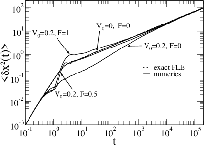
Figure 2: Anomalous diffusion in the potential $U(x)=-V_{0}\sin(2\pi x/L)-Fx$ for various $V_{0}$ and $F$ at $T=0.1$ for $\alpha=0.5$. Notice an excellent agreement (differences practically cannot be detected in this plot) of simulations with the exact FLE result, $\langle\delta x^{2}(t)\rangle=2v_{T}^{2}t^{2}E_{2-\alpha,3}[-(t/\tau_{v})^{2-\alpha}]$, in the absence of periodic potential $V_{0}=0$. Scaling: time in $\tau_{v}=(m/\eta_{\alpha})^{1/(2-\alpha)}$, distance in $L$, energy in $m(L/\tau_{v})^{2}$, force in $mL/\tau_{v}^{2}$ and temperature in $mL^{2}/(\tau_{v}^{2}k_{B})$.

A proper fractal scaling of coefficients $k_{i}$ and $\eta_{i}$ with $i$ (see above) allows one to model viscoelastic subdiffusion over arbitrary time scales of the experimental interest. One can numerically solve these stochastic differential equations (IV.2) e.g. with a standard stochastic Heun methodGard (second order Runge-Kutta method) as done in Refs. Goychuk09 ; G10 . An example of such simulations is given in Figs. 2, 3 for $\alpha=0.5$, $\nu_{0}=100$, $b=10$, $C_{\alpha}(b)=1.3$, $N=12$ and $k_{B}T=0.1$. The following scaling is used: time in the units of $\tau_{v}$ , distance in the units of $L$. All the energy units are then scaled in $\Delta E=m(L/\tau_{v})^{2}$ and the force units in $mL/\tau_{v}^{2}$. Stochastic Heun method is used to integrate Eq. (IV.2) with a time step $\Delta t=(1-5)\cdot 10^{-3}$ until $t_{\rm max}=2\cdot 10^{5}$ and $n=10^{4}$ trajectories are used for the ensemble averaging. Stochastic numerics are compared against the exact results for the free subdiffusion and for the mean displacement under a constant biasing force. The agreement is excellent. The considered particular embedding still works as an approximation to the FLE dynamics until $t=10^{8}$. If one needs to describe subdiffusion on an even longer time scale one can increase $N$. If one needs a better precision of approximation one can make $b$ smaller. Initially all the particles are localized at the origin, $x=0$, with the velocities thermally distributed at the temperature $T$. For the time span $t\lesssim\tau_{v}$ the motion is always ballistically persistent (superdiffusion). This reflects the inertia of the Brownian particle. It assumes the subdiffusive character for $t\gg\tau_{v}$, when the VACF is negative. The presence of a periodic potential $V(x)=-V_{0}\sin(2\pi x/L)$ dramatically changes both subdiffusion, $\langle x^{2}(t)\rangle-\langle x(t)\rangle^{2}$, as well as subdiffusive transport, $\langle x(t)\rangle$, on intermediate time scale. However, the long time asymptotics of free or biased subdiffusion are gradually attained. The initial behavior still within one potential well remains ballistic. One can conclude that both subdiffusion and subdiffusive transport are indeed asymptotically insensitive to the presence of periodic potential within the GLE approach. This finding is in a striking contrast with the FFPE approach. However, the transient to this asymptotic regime can be very slow, depending on the amplitude of the periodic potential and temperature.

An interesting phenomenon is also accelerated subdiffusion occurring on an intermediate time scale in tilted washboard potentials, as compared with the free subdiffusion. It can be detected in Fig. 2 for a strong yet subcritical bias $F=1<F_{\rm cr}=2\pi V_{0}/L\approx 1.2566...$. This calls to mind the acceleration of normal diffusion in tilted washboard potentialsReimann3 . However, this accelerated subdiffusive phenomenon occurs only on an intermediate time scale because asymptotically the GLE subdiffusion is not sensitive to the presence of the potential. One more interesting effect occurs for the initially ballistic transport. It first seems paradoxical that in the trapping potential the initial transport becomes faster than in the absence of potential and not vice versa, see in Fig. 3. The result can be understood in view of the fact that the minimum of the potential under the strong bias $F$ is essentially displaced in the direction of biasing force and the particles are initially accelerated by the additional to $F$ force stemming from the periodic potential.

Figure 3: Anomalous transport for $F>0$, see Fig.2 for details.

V Summary and conclusions

With this Chapter, we reviewed and scrutinized two different approaches, the FFPE approach and the FLE approach, to anomalously slow diffusion and transport in nonlinear force fields with a focus on applications in tilted periodic potentials. In spite of some similarities in the case of constant or linear forcings it was shown that the nonlinear dynamics radically differ, obeying asymptotically two different universality classes. A first one reflects the universal fluctuations of intrinsic time clock and is closely tight to a weak ergodicity breaking. In contrast, within the GLE and FLE approach the long-range antipersistence of the velocity and position fluctuations renders the asymptotic dynamics ergodic. One approach seems more appropriate for the disordered solids, or glass-forming liquids below the glass-forming transition, as characterized by the nonergodic glass phase. Another one seems more appropriate for the regime above but close to the glass transition, or for crowded viscoelastic environments like cytosols in biological cells. We have left out further pronounced differences between the FFPE and FLE approaches in the case of time-dependent fieldsSK06 ; HPRL07 ; G07 ; H09 ; West2 . We are confident that our results not only shed light on the origin of profound differences, but also will stimulate a further development of both approaches to subdiffusion, and possibly other interrelationships emerging in random potentials.

Appendix A Continuous time random walk and random clock

Consider a lattice with period $a$ and a particle jumping with probabilities $q_{+}$ and $q_{-}$, $q_{+}+q_{-}=1$, to the neighboring sites after a random clock characterized by the residence time distribution (RTD) $\psi(\tau)$ “ticked” on the next jump. Within the physical time interval $t$ there will be a variable random number of intrinsic time periods $n(t)$. The probability to make $m$ steps forward and $n-m$ steps backward after $n$ periods is given by the binomial distribution, $P(m,n)=n!/[m!(n-m)!]q_{+}^{m}q_{-}^{n-m}$. Using it one can calculate the first two moments, $\langle x^{k}\rangle=a^{k}\sum_{m=0}^{n}(2m-n)^{k}P(m,n),k=1,2$, of the particle displacement after $n$ periods:

$$\langle x(t)\rangle = a(q_{+}-q_{-})n(t)$$

$$\langle x^{2}(t)\rangle = a^{2}\left[n^{2}(t)(q_{+}-q_{-})^{2}+4n(t)q_{+}q_{-}\right]\;.$$ (32)

They are still random quantities because of the randomness of $n(t)$. Each particle has an individual number of periods completed until $t$. For the additional ensemble average one obtains

$$\langle\langle x(t)\rangle\rangle_{\rm ens} = a(q_{+}-q_{-})\langle n(t)\rangle_{\rm ens}$$

$$\langle\langle x^{2}(t)\rangle\rangle_{\rm ens} = a^{2}\left[\langle n^{2}(t)\rangle_{\rm ens}(q_{+}-q_{-})^{2}+4\langle n(t)\rangle_{\rm ens}q_{+}q_{-}\right]\;$$ (33)

and for the ensemble-averaged variance $\langle\langle[x-\langle\langle x\rangle\rangle_{\rm ens}]^{2}\rangle\rangle_{\rm ens}=\langle\langle x^{2}\rangle\rangle_{\rm ens}-\langle\langle x\rangle\rangle^{2}_{\rm ens}$

$$\langle\langle\delta x^{2}(t)\rangle\rangle_{\rm ens} = a^{2}\left[\langle\delta n^{2}(t)\rangle_{\rm ens}(q_{+}-q_{-})^{2}+4\langle n(t)\rangle_{\rm ens}q_{+}q_{-}\right]\;$$ (34)

where $\langle\delta n^{2}(t)\rangle_{\rm ens}=\langle n^{2}(t)\rangle_{\rm ens}-\langle n(t)\rangle_{\rm ens}^{2}$ is the variance of random periods passed. Notice that $\langle\langle x^{2}\rangle\rangle_{\rm ens}-\langle\langle x\rangle\rangle^{2}_{\rm ens}\neq\langle\langle[x-\langle x\rangle]^{2}\rangle\rangle_{\rm ens}$. Clearly, for a regular clock, $\langle\delta n^{2}(t)\rangle_{\rm ens}=0$ and the corresponding contribution to the ensemble-averaged position variance is absent. To simplify the notations, we further denote the ensemble averages as $\langle...\rangle$ rather than $\langle\langle...\rangle\rangle_{\rm ens}$.

The physical time $t$ can be measured by the sum of independent stochastic periods $\tau_{k}$ already completed and one not yet completed period $\tau_{n+1}^{*}$, $t=\sum_{k=1}^{n(t)}\tau_{k}+\tau_{n+1}^{*}$, with $n=0,1,2,...,\infty$. Therefore, the probability distribution $p(n,t)$ to have $n$ time periods within $t$, $\sum_{n=0}^{\infty}p(n,t)=1$, is the $n+1$-time convolution of the RTDs $\psi(\tau)$ ($n$ times) and of the survival probability $\Phi(\tau)=\int_{\tau}^{\infty}\psi(\tau)d\tau$. Its Laplace-transform reads

$$\tilde{p}(n,s)=\frac{1-\tilde{\psi}(s)}{s}[\tilde{\psi}(s)]^{n}$$ (35)

in terms of the Laplace-transformed $\psi(\tau)$. Let’s consider $\tilde{\psi}(s)\approx 1-(s\tau_{\rm sc})^{\alpha}$ for $s\tau_{\rm sc}\to 0$, where $\tau_{\rm sc}$ is a time unit of measurements. The continuous spatial limit is achieved when $a\to 0$, $\tau_{\rm sc}\to 0$ with $\kappa_{\alpha}=a^{2}/\tau_{\rm sc}^{\alpha}$ being a constant. For a finite $\tau_{\rm sc}$, considering the scaling limit $n\to\infty$, $s\tau_{\rm sc}\to 0$ with $n(s\tau_{\rm sc})^{\alpha}$ being finite, one obtains

$$\tilde{p}(n,s)=\tau_{\rm sc}(s\tau_{\rm sc})^{\alpha-1}\exp[-n(s\tau_{\rm sc})^{\alpha}],$$ (36)

where $n$ is considered as a continuous variable and

$$\tau(t)=n(t)\tau_{\rm sc}$$ (37)

is the intrinsic random time. Notice that for $\alpha=1$ one finds, $p(n,t)=\delta(n-t/\tau_{\rm sc})$ by inversion to the time domain. That means to say that $\tau(t)=t$ is not random. For $0<\alpha<1$, $p(n,t)$ can be expressed via the one-sided Levy distribution density ${\cal L}_{\alpha}(t)$ whose Laplace transform reads $\tilde{\cal L}_{\alpha}(s)=\exp(-s^{\alpha})$. Then, all the moments $\langle n^{k}(t)\rangle$ can be easily found from (36) to read

$$\langle n^{k}(t)\rangle=\frac{\Gamma(1+k)}{\Gamma(1+k\alpha)}(t/\tau_{\rm sc})^{k\alpha}.$$ (38)

In spite of the fact that the mean time interval $\langle\tau\rangle$ does not exist all the moments of the intrinsic time $\tau(t)$ are finite. This might seem paradoxical. However, the intrinsic time scales with the number of stochastic periods passed and if the mean period does not exist the moments of $n(t)$ are nevertheless finite for any finite $t$. This is because a frequent occurrence of very long stochastic time periods within some fixed $t$ implies a smaller value of $n(t)$. In particular,

$$\langle n(t)\rangle = (t/\tau_{\rm sc})^{\alpha}/\Gamma(1+\alpha),$$

$$\langle n^{2}(t)\rangle = 2(t/\tau_{\rm sc})^{2\alpha}/\Gamma(1+2\alpha),\;$$ (39)

and

$$\frac{\langle\delta n^{2}(t)\rangle}{\langle n(t)\rangle^{2}}=\frac{\langle\delta\tau^{2}(t)\rangle}{\langle\tau(t)\rangle^{2}}=\frac{2\Gamma^{2}(1+\alpha)}{\Gamma(1+2\alpha)}-1$$ (40)

is the most important property of the stochastic clock. It is primarily responsible for the discussed universality class of the CTRW-based subdiffusion associated with the universal fluctuations, and the weak ergodicity breaking.

References

- (1) M. F. Shlesinger, Asymptotic solutions of continuous time random walks, J. Stat. Phys. 10, 421–434 (1974).
- (2) H. Scher and E. M. Montroll, Anomalous transit time dispersion in amorphous solids, Phys. Rev. B 12, 2455–2477 (1975).
- (3) J.-P. Bouchaud and A. Georges, Anomalous diffusion in disordered media: statistical mechanisms, models and physical applications, Phys. Rep. 195, 127–293 (1990).
- (4) B. D. Hughes, Random walks and Random Environments, Vols. 1,2 (Clarendon Press, Oxford, 1995).
- (5) M. F. Shlesinger, Random processes, in: Encyclopedia of Applied Physics 16 (VCH Publishers, 1996), pp. 45–70.
- (6) R. Metzler and J. Klafter, The random walk’s guide to anomalous diffusion: a fractional dynamics approach, Phys. Rep. 339, 1–77 (2000).
- (7) B. J. West and W. Deering, Fractal physiology for physicists: Levy statistics, Phys. Rep. 246, 2–100 (1994).
- (8) B. J. West, E. L. Geneston, and P. Grigolini, Maximizing information exchange between complex networks, Phys. Rep. 468, 1–99 (2008).
- (9) G. M. Zaslavsky, Chaos, fractional kinetics, and anomalous transport, Phys. Rep. 371, 461–580 (2002).
- (10) I. M. Sokolov, Statistics and the single molecule, Physics 1, 8 (2008).
- (11) M. J. Saxton and K. Jacobson, Single-particle tracking: applications to membrane dynamics, Annu. Rev. Biophys. Biomol. Struct. 26, 373–399 (1997).
- (12) G. Seisenberger, et al., Real-time single-molecule imaging of the infection pathway of an adeno-associated virus, Science 294, 1929–1932 (2001).
- (13) I. M. Tolić-Nørrelykke, et al., Anomalous diffusion in living yeast cells, Phys. Rev. Lett. 93, 078102 (2004).
- (14) I. Goychuk and P. Hänggi, Fractional diffusion modeling of ion channel gating, Phys. Rev. E 70, 051915 (2004).
- (15) I. Golding and E. C. Cox, Physical nature of bacterial cytoplasm, Phys. Rev. Lett. 96, 098102 (2006).
- (16) C. Wilhelm, Out-of-equilibrium microrheology inside living cells, Phys. Rev. Lett. 101, 028101 (2008).
- (17) F. Amblard, et al., Subdiffusion and anomalous local viscoelasticity in actin networks, Phys. Rev. Lett. 77, 4470–4473 (1996).
- (18) J. Szymanski and M. Weiss, Elucidating the origin of anomalous diffusion in crowded fluids, Phys. Rev. Lett. 103, 038102 (2009).
- (19) S. C. Kou and X. S. Xie, Generalized Langevin equation with fractional Gaussian noise: Subdiffusion within a single protein molecule, Phys. Rev. Lett. 93, 180603 (2004); W. Min, et al., Observation of a power-law memory kernel for fluctuations within a single protein molecule, Phys. Rev. Lett. 94, 198302 (2005).
- (20) D. Mizuno, C. Tardin, C. F. Schmidt, and F. C. MacKintosh, Nonequilibrium mechanics of active cytoskeletal networks, Science 315, 370–373 (2007).
- (21) R. Granek and J. Klafter, Fractons in proteins: Can they lead to anomalously decaying time autocorrelations? Phys. Rev. Lett. 95, 098106 (2005); S. Reuveni, R. Granek, and J. Klafter, Proteins: coexistence of stability and flexibility, Phys. Rev. Lett. 100, 208101 (2008); M. de Leeuw, et al. Coexistence of flexibility and stability of proteins: an equation of state, PLoS One 4, e7296 (2009).
- (22) G. Bel and E. Barkai, Weak ergodicity breaking in the continuous-time random walk, Phys. Rev. Lett. 94, 240602 (2005).
- (23) Y. He, S. Burov, R. Metzler and E. Barkai, Random time-scale invariant diffusion and transport coefficients, Phys. Rev. Lett. 101, 058101 (2008).
- (24) A. Lubelski, I. M. Sokolov, and J. Klafter, Nonergodicity mimics inhomogeneity in single particle tracking, Phys. Rev. Lett. 100, 250602 (2008)
- (25) J. Nelson, Continuous-time random-walk model of electron transport in nanocrystalline electrodes, Phys. Rev. B 59, 15374–15380 (1999).
- (26) R. Metzler, E. Barkai, J. Klafter, Anomalous diffusion and relaxation close to thermal equilibrium: A fractional Fokker-Planck equation approach, Phys. Rev. Lett. 82, 3563-3567 (1999).
- (27) E. Barkai, Fractional Fokker-Planck equation, solution, and application, Phys. Rev. E 63, 046118 (2001).
- (28) R. Gorenflo and F. Mainardi, in: Fractal and Fractal Calculus in Continuum Mechanics, ed. by A. Carpinteri and F. Mainardi (Springer, Wien, 1997), 223–276.
- (29) I. Goychuk, E. Heinsalu, M. Patriarca, G. Schmid, P. Hänggi, Current and universal scaling in anomalous transport, Phys. Rev. E 73, 020101 (Rapid Communication) (2006).
- (30) E. Heinsalu, M. Patriarca, I. Goychuk, G. Schmid, P. Hänggi, Fractional Fokker-Planck dynamics: Numerical algorithm and simulations, Phys. Rev. E 73, 046133 (2006).
- (31) P. Hänggi and H. Thomas, Time Evolution, Correlations and Linear Response of Non-Markov Processes Z. Physik B 26, 85–92 (1977).
- (32) H. Grabert, P. Hänggi, and P. Talkner, Microdynamics and nonlinear stochastic processes of gross variables, J. Stat. Phys. 22, 537–552 (1980).
- (33) B. B. Mandelbrot and J. W. van Ness, Fractional Brownian motions, fractional noises and applications, SIAM Review 10, 422 (1968).
- (34) I. Goychuk, Viscoelastic subdiffusion: from anomalous to normal, Phys. Rev. E 80, 046125 (2009).
- (35) J. H. Jeon and R. Metzler, Fractional Brownian motion and motion governed by the fractional Langevin equation in confined geometries, Phys. Rev. E 81, 021103 (2010).
- (36) J. C. Maxwell, On the dynamical theory of gases, Phil. Trans. R. Soc. Lond. 157, 49–88 (1867).
- (37) A. Gemant, A method of analyzing experimental results obtained from elasto-viscous bodies, Physics 7, 311–317 (1936).
- (38) T. G. Mason and D. A. Weitz, Optical measurements of frequency-dependent linear viscoelastic moduli of complex fluids, Phys. Rev. Lett. 74, 1250–1253 (1995).
- (39) F. C. MacKintosh, C. F. Schmidt, Microrheology, Curr. Opin. Coll. Interface Sci. 4, 300–307 (1999).
- (40) P. Reimann, A uniqueness-theorem for “linear” thermal baths, Chem. Phys. 268, 337–346 (2001).
- (41) E. Lutz, Fractional Langevin equation, Phys. Rev. E 64, 051106 (2001).
- (42) W. T. Coffey, Y. P. Kalmykov, J. T. Waldron, The Langevin Equation: With Applications to Stochastic Problems in Physics, Chemistry and Electrical Engineering, 2nd ed. (World Scientific, Singapore, 2004).
- (43) I. Goychuk and P. Hänggi, Anomalous escape governed by thermal 1/f noise, Phys. Rev. Lett. 99, 200601 (2007).
- (44) S. Burov and E. Barkai, Critical exponent of the fractional Langevin equation, Phys. Rev. Lett. 100, 070601 (2008).
- (45) R. Kubo, The fluctuation-dissipation theorem, Rep. Prog. Phys. 29, 255 (1966).
- (46) R. Kubo, M. Toda, and M. Hashitsume, Nonequilibrium Statistical Mechanics, 2nd ed. (Springer, Berlin, 1991).
- (47) R. Zwanzig, Nonequilibrium Statistical Mechanics (Oxford University Press, Oxford, 2001).
- (48) P. Hänggi, P. Talkner, and B. Borkovec, Reaction-rate theory: fifty years after Kramers, Rev. Mod. Phys. 62, 251–341 (1990).
- (49) U. Weiss, Quantum Dissipative Systems, 2nd ed. (World Scientific, Singapore, 1999).
- (50) A. Taloni, A. Chechkin, J. Klafter, Generalized elastic model yields a fractional Langevin equation description, Phys. Rev. Lett. 104, 160602 (2010).
- (51) S. A. Adelman, Fokker-Planck equations for simple non-Markovian systems, J. Chem. Phys. 64, 124 (1976).
- (52) P. Hänggi, H. Thomas, H. Grabert, P. Talkner, Note on time evolution of non-Markov processes, J. Stat. Phys. 18, 155 (1978).
- (53) J. T. Hynes, Outer-sphere electron-transfer reactions and frequency-dependent friction, J. Phys. Chem. 90, 3701–3706 (1986).
- (54) H. C. Fogedby, Langevin-equations for continuous-time Levy flights, Phys. Rev. E 50, 1657–1660 (1994); A. A. Stanislavsky, Fractional dynamics from the ordinary Langevin equation, Phys. Rev. E, 67, 021111 (2003); M. Magdziarz, A. Weron, K. Weron, Fractional Fokker-Planck dynamics: Stochastic representation and computer simulation, Phys. Rev. E 75, 016708 (2007).
- (55) N. Pottier, Aging properties of an anomalously diffusing particle, Physica A 317, 371–382 (2003).
- (56) W. H. Deng, E. Barkai, Ergodic properties of fractional Brownian-Langevin motion, Phys. Rev. E 79, 011112 (2009).
- (57) I. M. Sokolov, E. Heinsalu, P. Hänggi, I. Goychuk, Universal fluctuations in subdiffusive transport, Europhys. Lett. 86, 30009 (2009).
- (58) M. Z. Ding, W. M. Yang, Distribution of the first return time in fractional Brownian motion and its application to the study of on-off intermittency, Phys. Rev. E 52, 207–213 (2005).
- (59) R. L. Stratonovich, Topics in the Theory of Random Noise, Vol. II (Gordon and Breach, New York, 1967).
- (60) P. Reimann, Brownian motors: noisy transport far from equilibrium, Phys. Rep. 361, 57–265 (2002).
- (61) P. Hänggi and F. Marchesoni, Artificial Brownian motors: Controlling transport on the nanoscale, Rev. Mod. Phys. 81, 387–442 (2009)
- (62) E. Heinsalu, M. Patriarca, I. Goychuk, and P. Hänggi, Fractional diffusion in periodic potentials, J. Phys.: Condens. Matt. 19, 065114 (2007).
- (63) E. Heinsalu, M. Patriarca, I. Goychuk, and P. Hänggi, Fractional Fokker-Planck subdiffusion in alternating force fields, Phys. Rev. E 79, 041137 (2009).
- (64) I. Goychuk, Subdiffusive Brownian ratchets rocked by a periodic force, Chem. Phys. 375, 450–457 (2010).
- (65) P. Hänggi and F. Mojtabai, Thermally activated escape rate in presence of long-time memory, Phys. Rev. A 26, 1168–1170 (1982).
- (66) Y. C. Chen and J. L. Lebowitz, Quantum particle in a washboard potential. I. Linear mobility and the Einstein relation, Phys. Rev. B46, 10743–10750 (1992).
- (67) M. Ferrario and P. Grigolini, The non-Markovian relaxation process as a “contraction” of a multidimensional one of Markovian type, J. Math. Phys.20, 2567 (1979); F. Marchesoni and P. Grigolini, On the extension of the Kramers theory of chemical relaxation to the case of nonwhite noise, J. Chem. Phys. 78, 6287 (1983).
- (68) R. Kupferman, Fractional kinetics in Kac-Zwanzig heat bath models, J. Stat. Phys. 114, 291 (2004).
- (69) P. Siegle, I. Goychuk, P. Talkner, and P. Hänggi, Markovian embedding of non-Markovian superdiffusion, Phys. Rev. E81, 011136 (2010).
- (70) R. G. Palmer, D. L. Stein, E. Abrahams, P. W. Anderson, Models of hierarchically constrained dynamics for glassy relaxation, Phys. Rev. Lett. 53, 958–961 (1984).
- (71) M. B. Weismann, 1/f noise and other slow, nonexponential kinetics in condensed matter, Rev. Mod. Phys.60, 537–571 (1988).
- (72) T. C. Gard, Introduction to Stochastic Differential Equations (Dekker, New York, 1988).
- (73) P. Reimann, C. Van der Broek, H. Linke, P. Hänggi, J. M. Rubi, A. Perez-Madrid, Giant acceleration of free diffusion by use of tilted periodic potentials, Phys. Rev. Lett. 87, 010602 (2001); ibid., Diffusion in tilted periodic potentials: enhancement, universality, and scaling, Phys. Rev. E 65, 031104 (2002).
- (74) I. M. Sokolov and J. Klafter, Field-induced dispersion in subdiffusion, Phys. Rev. Lett. 97, 140602 (2006).
- (75) E. Heinsalu, M. Patriarca, I. Goychuk, and P. Hänggi, Use and abuse of a fractional Fokker-Planck dynamics for time-dependent driving, Phys. Rev. Lett. 99, 120602 (2007).
- (76) I. Goychuk, Anomalous relaxation and dielectric response, Phys. Rev. E 76, 040102(R) (2007).