The rapid X-ray variability of NGC 4051

Abstract

We present an analysis of the high frequency X-ray variability of NGC 4051 ($M_{\rm BH}\sim 1.7\times 10^{6}$ $\rm\thinspace M_{\odot}$) based on a series of XMM-Newton observations taken in 2009 with a total exposure of $\sim 570$ ks (EPIC pn). These data reveal the form of the power spectrum over frequencies from $10^{-4}$ Hz, below the previously detected power spectral break, to $\mathrel{\hbox{\hbox to0.0pt{\hbox{\lower 4.0pt\hbox{$\sim$}}\hss}\hbox{$>$}}}10^{-2}$ Hz, above the frequency of the innermost stable circular orbit (ISCO) around the black hole ($\nu_{\rm ISCO}\sim 10^{-3}-10^{-2}$ Hz, depending on the black hole spin parameter $j$). This is equivalent to probing frequencies $\mathrel{\hbox{\hbox to0.0pt{\hbox{\lower 4.0pt\hbox{$\sim$}}\hss}\hbox{$>$}}}1$ kHz in a stellar mass ($M_{\rm BH}\sim 10$ $\rm\thinspace M_{\odot}$) black hole binary system. The power spectrum is a featureless power law over the region of the expected ISCO frequency, suggesting no strong enhancement or change in the variability at the fastest orbital period in the system. Despite the huge amplitude of the flux variations between the observations (peak-to-peak factor of $\mathrel{\hbox{\hbox to0.0pt{\hbox{\lower 4.0pt\hbox{$\sim$}}\hss}\hbox{$>$}}}50$) the power spectrum appears to be stationary in shape, and varies in amplitude at all observed frequencies following the previously established linear rms-flux relation. The rms-flux relation is offset in flux by a small and energy-dependent amount. The simplest interpretation of the offset is in terms of a very soft spectral component that is practically constant (compared to the primary source of variability). One possible origin for this emission is a circumnuclear shock energised by a radiatively driven outflow from the central regions, and emitting via inverse-Compton scattering of the central engine’s optical-UV continuum (as inferred from a separate analysis of the energy spectrum). A comparison with the power spectrum of a long XMM-Newton observation taken in 2001 gives only weak evidence for non-stationarity in power spectral shape or amplitude. Despite being among the most precisely estimated power spectra for any active galaxy, we find no strong evidence for quasi-periodic oscillations (QPOs) and determine an upper limit on the strength of a plausible QPO of $\mathrel{\hbox{\hbox to0.0pt{\hbox{\lower 4.0pt\hbox{$\sim$}}\hss}\hbox{$<$}}}2$ per cent rms in the $3\times 10^{-3}-0.1$ Hz range, and $\sim 5-10$ per cent in the $10^{-4}-3\times 10^{-3}$ Hz range. We compare these results to the known properties of accreting stellar mass black holes in X-ray binaries, with the aim further of developing a ‘black hole unification’ scheme.

1 Introduction

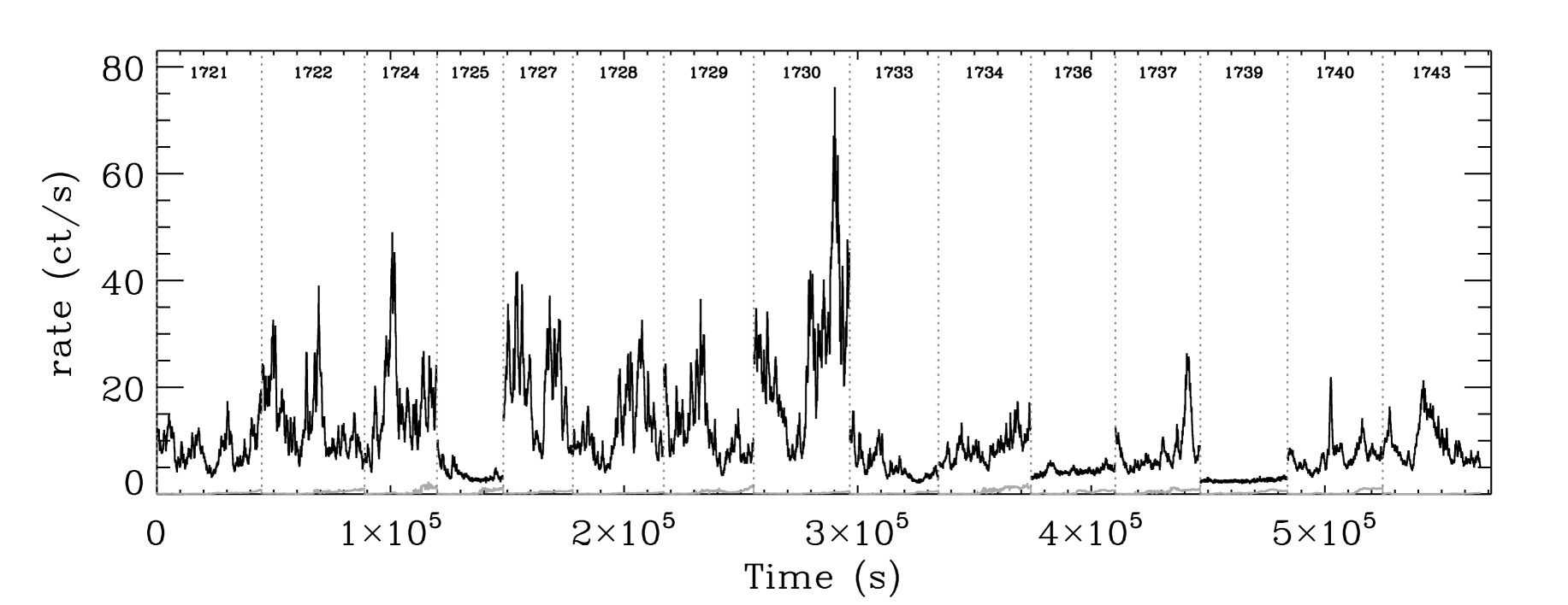
Figure 1: Time series of $0.2-10$ keV EPIC pn count rate (background-subtracted) from each of the $15$ observations taken in 2009. The bin size is $\Delta t=100$ s. The $15$ separate $\sim 30-40$ ks observations, taken typically $~{}2-4$ days apart, have been concatenated in this plot, to allow easy comparison between them, with the end points marked by the dotted vertical line. The background count rate is also shown as a grey curve, but is almost always far weaker than the source. The labels above each section of data refer to the spacecraft revolutions during which the observations were made.

If strong gravity dominates the dynamics of the inner accretion flows around black holes then an elementary consequence is scale invariance: many important aspects of accretion onto supermassive black holes ($M_{\rm BH}\mathrel{\hbox{\hbox to0.0pt{\hbox{\lower 4.0pt\hbox{$\sim$}}\hss}\hbox{$>$}}}10^{6}$ $\rm\thinspace M_{\odot}$) in Active Galactic Nuclei (AGN) should be fundamentally the same as for stellar mass black holes ($M_{\rm BH}\sim 10$ $\rm\thinspace M_{\odot}$) in Galactic Black Hole systems (GBHs). (See e.g. Shakura & Sunyaev 1976 and Mushotzky et al. 1993.) Over the past few years several similarities have been observed in the X-ray variability of nearby AGN and GBHs, supporting the idea of black hole unification (Fender et al., 2006). In particular, the power spectrum (often power spectral density, PSD), and inter-band X-ray time lags appear to have similar frequency dependence and relative amplitudes in AGN and GBHs but with characteristic frequencies scaled (to first order) inversely with mass, $\nu\propto 1/M_{\rm BH}$ (see e.g. Lawrence et al., 1987; Hayashida et al., 1998; Edelson & Nandra, 1999; Uttley et al., 2002; Vaughan et al., 2003; Markowitz et al., 2003; M^cHardy et al., 2004; Done & Gierliński, 2005; M^cHardy et al., 2006; M^cHardy et al., 2007; Gierliński et al., 2008; Arévalo et al., 2008). Another property of the X-ray variability common to both types of system is a linear rms-flux relation, a scaling of the rms amplitude of variability with average source flux that appears to hold over a very wide range of timescales (Uttley & M^cHardy, 2001; Vaughan et al., 2003; Gaskell, 2004; Gleissner et al., 2004; Uttley et al., 2005).

Arguably among the most important recent breakthroughs in the study of stellar mass black holes was the discovery of quasi-periodic oscillations (QPOs) at high frequencies ($\nu_{\rm Q}\mathrel{\hbox{\hbox to0.0pt{\hbox{\lower 4.0pt\hbox{$\sim$}}\hss}\hbox{$>$}}}100$ Hz) in GBHs (see Remillard et al., 1999; Strohmayer, 2001; Remillard et al., 2002, 2003; van der Klis, 2006; Remillard & McClintock, 2006). These are the fastest variations observed from GBHs and their high frequencies, close to the Keplerian frequency of the innermost stable circular orbit (ISCO; $\nu_{\rm ISCO}$), indicate an origin in the central regions of the accretion flow. High frequency QPOs (HF QPOs) therefore carry information on the strongly curved spacetime close to the event horizon and should, in principle, constrain the fundamental parameters of black holes: mass and spin. As a product of strong gravity, HF QPOs should also be present in AGN, but until recently there were no robust detections, due mainly to the insufficient length of previous XMM-Newton observations (see Vaughan & Uttley, 2005, 2006). Recently a QPO was detected in the Seyfert galaxy RE J1034+396 (Gierliński et al., 2008). This is a major discovery that adds further support to the general idea that AGN are scaled-up GBHs, but this one detection provides limited diagnostic power because it is so far unique and the other properties of the source are not well understood (Middleton et al., 2009; Middleton & Done, 2010)

In parallel with these X-ray advances, studies of transient radio jets from GBHs have led to the development of a scheme that unifies jet production with accretion state (Fender et al., 2004). Relativistic jets must be launched from the region dominated by strong-field gravity, and so scale invariance implies this accretion state/jet unification scheme should extend to AGN (Heinz & Sunyaev, 2003), a hypothesis supported by observations (Merloni et al., 2003; Falcke et al., 2004; Körding et al., 2006). From these results a new paradigm is emerging in which accretion mode, X-ray spectrum, high-frequency timing properties and jet production for both GBH “states” and AGN “types” may be unified into a single framework for the activity cycles of accreting black holes.

Here we discuss the results obtained from a series of XMM-Newton observations of the bright, highly-variable Seyfert 1 galaxy NGC 4051. These observations were designed to provide some of the best constraints to date on the high-frequency X-ray variability properties of any AGN and improve our understanding of black hole unification generally. This particular target was chosen because of a combination of factors. NGC 4051 (redshift $z=0.002336$, distance $D\approx 15$ Mpc; Russell, 2002) has a relatively low and well-determined black hole mass, $M_{\rm BH}\approx 1.7\pm 0.5\times 10^{6}~{}\hbox{$\rm\thinspace M_{\odot}$}$ (Denney et al., 2009, 2010), displays strong, persistent X-ray flux and spectral variability (see e.g. Lawrence et al., 1987; Papadakis & Lawrence, 1995; M^cHardy et al., 2004; Uttley et al., 2004; Ponti et al., 2006; Terashima et al., 2009), and a soft X-ray spectrum rich in emission and absorption features (Collinge et al., 2001; Pounds et al., 2004; Ogle et al., 2004; Steenbrugge et al., 2009).

2 Observations and data analysis

NGC 4051 was observed by XMM-Newton $15$ times over $45$ days during May-June 2009, and previously during 2001 and 2002 (see table 1). The total duration of the useful data from the 2009 campaign is $\approx 572$ ks, giving $\sim 6\times 10^{6}$ EPIC pn source counts (using PATTERN $0-4$) or $\sim 9\times 10^{6}$ EPIC source counts (using PATTERN $0-12$ pn and MOS combined).

The raw data were processed from Observation Data Files (ODFs) following standard procedures using the XMM-Newton Science Analysis System (SAS v10.0.2). The EPIC data were processed using the standard SAS processing chains to produce calibrated event lists. For each observation, source events were extracted from these using a $40$ arcsec circular region centred on the the target, and background events were extracted from a rectangular region on the same chip but not overlapping with the source region. (In order to obtain a precise background estimate the background region was $\sim 7$ times larger than the source region.) Examination of the background time series showed the background to be relatively low and stable throughout most of the observations, with the exception of the final few ks of each observation where the background rate increased as the spacecraft approached the radiation belts at perigee (each of the observations occurred towards the end of a spacecraft revolution). The EPIC data were taken using the small window mode of each camera and the medium blocking filter to reduce pile-up and optical loading effects, respectively. Nevertheless, during bright intervals NGC 4051 is sufficiently bright to cause moderate pile-up, especially in the MOS, which can affect power spectrum estimation (Tomsick et al., 2004). In order to mitigate any distorting effects all results are based on pn data PATTERNS $0-4$ only, but where possible checked for consistency with the MOS data. Response matrices were generated using RMFGEN v1.55.2 and ancillary responses were generated with ARFGEN v.1.77.4.

Table 1: Observation log. The columns list (1) the observation identifier, (2) the spacecraft revolution number, (3) the date of the start of the observation, (4) the observation duration.

Obs ID.		Obs. date	Duration
ID	rev.	(YYYY-MM-DD)	(ks)
0109141401	0263	2001-05-16	121958
0157560101	0541	2002-11-22	51866
0606320101	1721	2009-05-03	45717
0606320201	1722	2009-05-05	45645
0606320301	1724	2009-05-09	45548
0606320401	1725	2009-05-11	45447
0606321301	1727	2009-05-15	32644
0606321401	1728	2009-05-17	42433
0606321501	1729	2009-05-19	41813
0606321601	1730	2009-05-21	41936
0606321701	1733	2009-05-27	44919
0606321801	1734	2009-05-29	43726
0606321901	1736	2009-06-02	44946
0606322001	1737	2009-06-04	39756
0606322101	1739	2009-06-08	43545
0606322201	1740	2009-06-10	44453
0606322301	1743	2009-06-16	42717

Time series were extracted from the filtered events for the source and background regions using a range of time bin sizes and energy ranges. These were all corrected for exposure losses, as catalogued in the Good Time Information (GTI) header contained in each event file, except where less than $30$ per cent of a bin was exposed, in which case the data were calculated by linear interpolation from the nearest ‘good’ data either side and appropriate Poisson noise was added (this was needed for only $0.3$ per cent of the total exposure time from the pn, for $\Delta t=5$ s time bins). The outputs of this process were regularly sampled and uninterrupted, exposure-corrected time series for source and background. The background time series was then subtracted from the corresponding source time series (after scaling by the ratio of the ‘good’ extraction region areas). Figure 1 shows the resulting time series from the $15$ separate 2009 observations.

3 Power spectrum

The power spectrum of the 2009 data was estimated using standard methods (van der Klis, 1989). In particular, time series were extracted with binning $\Delta t=5$ s and divided into uninterrupted $10$ ks intervals. For each interval a periodogram was computed in units of relative power (Miyamoto et al., 1991; van der Klis, 1997; Vaughan et al., 2003), the Poisson noise level was subtracted, and then the periodgrams were averaged. Figure 2 shows the resulting power spectrum estimate after rebinning in logarithmic frequency intervals. The model fitting was performed using XSPEC v12.6.0 (Arnaud, 1996) using $\chi^{2}$ as the fit statistic, all data were binned to ensure that Gauss-normal statistics applied, and errors quoted correspond to $90$ per cent confidence limits (e.g. using a $\Delta\chi^{2}=2.71$ criterion for one parameter) unless otherwise stated.

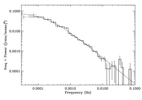
Figure 2: Power spectrum estimate (histogram) for the broad band ($0.2-10$ keV) EPIC pn data, computed using $10$ ks intervals at $\Delta t=5$ bins, with best-fitting bending power law continuum model (solid curve). Also shown (grey circles) are two low frequency power density estimates computed using $28$ ks intervals. These lower frequency data were not used in the fitting (see text for details).

The previous analysis of the power spectrum of NGC 4051 by M^cHardy et al. (2004) found a smoothly bending power law continuum provided an adequate description of the data

$$cont(\nu)=\frac{N\nu^{\alpha_{\rm low}}}{1+(\nu/\nu_{\rm bend})^{\alpha_{\rm low}-\alpha_{\rm high}}},$$ (1)

with indices of $\alpha_{\rm low}\approx-1.1$ at low frequencies and $\alpha_{\rm high}\approx-2$ above $\nu_{\rm bend}\sim 8\times 10^{-4}$ Hz. This model provided an excellent fit to the 2009 power spectrum, as shown in Figure 2, with the lower frequency index fixed at $\alpha_{\rm low}=-1.1$ (since it is much better constrained by the RXTE data; M^cHardy et al., 2004). The best-fitting values for the free parameters of the model were $\alpha_{\rm high}=-2.31\pm 0.08$ and $\nu_{\rm bend}=2.3\pm 1.0\times 10^{-4}$ Hz. The fit statistic was $\chi^{2}=31.19$ with $27$ degrees of freedom (dof), giving a $p$-value of $0.26$. Allowing $\alpha_{\rm low}$ to vary provided no improvement in the fit ($\Delta\chi^{2}<2$) and the index itself was poorly constrained (with a $90$ per cent confidence interval of $[-0.25,-1.78]$), and restricting $\alpha_{\rm low}$ to vary only within the range $[-1.2,-0.9]$ (the confidence interval determined by M^cHardy et al. (2004) from the RXTE data) provided very little change in the confidence interval for $\nu_{\rm bend}$ compared to the fixed $\alpha_{\rm low}=-1.1$ model. There is no obvious indication, in either the overall fit statistic or the residual plot, of additional power spectral components. We discuss this point in more detail in Section 5.

A sharply broken power law model also provided a good fit, with $\chi^{2}=37.52$ for $27$ dof ($p=0.086$), slightly worse than the smoothly bending model. The index below the break was again fixed to $\alpha_{\rm low}=-1.1$, and the best-fitting break frequency was $\nu_{\rm break}=2.5\pm 0.6\times 10^{-4}$ Hz, and a high frequency index of $\alpha_{\rm high}=-2.18\pm 0.05$. These parameters, and the overall fit quality, are very similar to those of the bending power law model, indicating that the data are rather insensitive to the detailed shape of the change from flat to steep index. By contrast, the power spectrum is less well explained in terms of an exponentially cut-off power law, which gives $\chi^{2}=44.03$ for $26$ dof ($p=0.015$), but only by allowing $\alpha_{\rm low}\approx-1.8$ which is inconsistent with the long-term RXTE results (M^cHardy et al., 2004). Assuming $\alpha_{\rm low}=1.1$ gave an unacceptable fit ($\chi^{2}=217.81$ for $27$ dof; $p\ll 0.001$).

The model fitting was repeated using a Bayesian scheme by treating the likelihood function as $\sim\exp(-\chi^{2}/2)$ and assigning simple prior distributions to the parameters. See Vaughan (2010), and references therein, for a brief introduction to these ideas. Uniform priors were assigned to $\alpha_{\rm high}$ and the overall normalisation, and to $\log\nu_{\rm bend}$ (equivalent to a $p(\nu)=1/\nu$ Jeffreys’ prior), although in practice using uniform or Jeffreys’ prior made no significant difference to the results. As expected, the parameter values at the posterior mode were almost identical to those giving the best-fit using the classical $\min\chi^{2}$ method. But having the problem restated in Bayesian terms allowed for an exploration of the posterior distribution of the parameters, $p(\theta_{C}\mid\mathbf{x}^{\rm obs})$ with $\theta_{C}$ the parameters specifying the continuum and $\mathbf{x}^{\rm obs}$ the observed data, using a Markov Chain Monte Carlo (MCMC) scheme to randomly draw sets of parameters from the posterior. The marginal density for the bend frequency, $p(\nu_{\rm bend}\mid\mathbf{x}^{\rm obs})$, as computed using the MCMC data, is shown in Figure 3; the $90$ per cent credible interval on $\nu_{\rm bend}$ was $[1.3,3.2]\times 10^{-4}$ Hz.

Figure 3: Marginal posterior probability density for the bend frequency in the bending power law model, computed by MCMC (see text for details). That for the 2009 data is shown as a solid curve, and that for the 2001 data is shown as the dashed curve.

The limited durations of the individual 2009 observations makes it difficult to directly probe frequencies lower than $10^{-4}$ Hz. But for completeness the power spectrum was also estimated using longer uninterrupted intervals ($28$ ks duration, of which there were $15$ in 2009, one for each observation). However, the estimates of power density at the lowest frequencies were not normally distributed in this case, due to the small number of estimates contributing to the average (Papadakis & Lawrence, 1993). These data were not included in the power spectral fitting, but the lowest frequency points are shown in Figure 2 and are clearly consistent with an extrapolation of the best-fitting model.

As a test for a possible high frequency cut-off in the power spectrum the bending power law model was modified by including an exponential cut-off (the highecut model in XSPEC). This provided only a very small improvement in the overall fit statistic ($\Delta\chi^{2}=4.1$ for $2$ additional free parameters) with only poorly constrained parameters (cut-off frequency $\nu_{\rm cut}\leq 8\times 10^{-3}$ and $e$-folding frequency $\nu_{\rm fold}=2\pm 1\times 10^{-2}$). The power spectrum estimated from the high flux data (see next section) has slightly higher signal-to-noise above $10$ mHz, but again shows no significant difference in the quality of the fit between the bending power law with and without an exponential cut-off at high frequencies.

3.1 Energy dependence of the power spectrum

The dependence of the power spectrum on photon energy was investigated by dividing the data into three broad energy bands – $0.2$–$0.7$, $0.7$–$2$ and $2$–$10$ – and estimating and fitting the power spectrum for each of these. A simultaneous fit to all these spectra using the same continuum model (equation 1) gave a rather poor fit ($\chi^{2}=118.9$ with $85$ dof, $p=0.009$) with the parameters tied between the three spectra. But allowing to be different for each energy band, while keeping $\nu_{\rm bend}$ tied between them, gave a much better fit ($\chi^{2}=98.5$ with $83$ dof, $p=0.12$); the improvement is significant in an $F$-test, with $p<0.001$, indicating the high frequency power spectrum is energy dependent. The slopes estimated for the low, medium and high energy bands were $2.31\pm 0.07$, $2.24\pm 0.09$ and $2.04\pm 0.10$, respectively. The flattening of the power spectrum at higher energies is very similar to that detected by M^cHardy et al. (2004) from the 2001 data, and previously observed in several other Seyfert galaxies (e.g. Nandra & Papadakis, 2001; Vaughan & Fabian, 2003). Allowing the bend frequency $\nu_{\rm bend}$ to be different for each energy band, but with $\alpha_{\rm high}$ tied between them, provided a considerably worse fit ($\chi^{2}=108.0$ with $83$ dof) than the energy-dependent $\alpha_{\rm high}$ model. Furthermore, allowing both $\nu_{\rm bend}$ and $\alpha_{\rm high}$ to differ between energy bands did not improve significantly on the variable $\alpha_{\rm high}$ fit ($\chi^{2}=95.7$ with $81$ dof). In this case the best-fitting $\nu_{\rm bend}$ values for the low and medium energy bands were very similar while the hard band gave a somewhat lower value, but with a much larger confidence interval. We conclude there is strong evidence for a change in the high frequency slope with energy, but the data do not resolve any difference in the location of the bend.

4 rms-flux relation

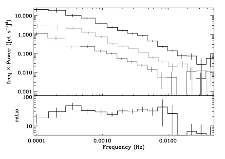
Figure 4: Power spectrum estimates computed as in Figure 2 from $10$ ks intervals but averaged into three flux bins, with average ($0.2-10$ keV pn) count rates of $4.8$, $8.4$ and $17.4$ ct s^-1. The lower panel shows the ratio of highest to lowest flux power spectral estimates, which is consistent with a constant over two decades in frequency, indicating a strong increase in absolute power but no strong change in shape with average flux. The data were binned logarithmically in frequency, by a factor $1.4$, and the bin centres shifted slightly to prevent the error bars overlapping.

The $15$ observations shown in Figure 1 clearly show very different mean levels and amplitudes of variability, with noticeably stronger variations occurring preferentially during brighter intervals (e.g. rev1730), and the lowest flux intervals being extremely stable (e.g. rev1739). This behaviour is exactly as expected for sources that obey the rms-flux relation (Uttley & M^cHardy, 2001; Uttley et al., 2005).

In order to test this explicitly and in detail the power spectrum was estimated in different flux bins. As before, the time series were divided into uninterrupted $10$ ks intervals, the periodograms computed and the contribution of the Poisson noise subtracted, but using absolute units of power (i.e. without normalising to the squared mean rate, see Vaughan et al., 2003). The intervals were sorted according to their mean flux, and the periodograms were then averaged in flux bins to provide estimates of the power spectrum as a function of mean flux. Figure 4 shows the power spectral estimates when the data were divided into three flux bins. There is clearly a large difference in the overall amplitude (in absolute units) but little change in shape, as revealed by the ratio of bright and faint power spectra. Direct fitting of the high and low flux power spectra gives the same result: the best-fitting values for $\alpha_{\rm high}$ and $\nu_{\rm bend}$ estimated for the high flux data fall within the $90$ per cent confidence intervals derived from the low flux data. The same effect was seen in Cygnus X-1 by Uttley & M^cHardy (2001) (see their figure $2$), and is consistent with there being a single rms-flux relation independent of the frequencies used to compute the rms.

The detailed rms-flux relation was then examined explicitly by dividing the data into $1$ ks uninterrupted intervals, computing a periodogram for each (again, in absolute units), subtracting the Poisson noise from each, and then averaging the results in several flux bins ($F_{i}$). The $1-10$ mHz rms, $\sigma_{i}$ was then estimated for each flux bin by integrating the corresponding power spectrum estimate over this frequency range. The resulting rms-flux data are shown in Figure 5. (The uncertainties on the rms estimates were calculated based on the variance of the sum of the averaged periodograms, which are themselves calculated based on the chi-square distribution of periodogram ordinates. The method is explained more fully in Heil, Vaughan & Uttley in prep.)

The dependence of rms on flux is clearly very close to linear over the full flux range, as previously noted in this source and accreting black holes generally (e.g. Uttley & M^cHardy, 2001; Uttley et al., 2005, Heil, Vaughan & Uttley in prep.). The best-fitting linear function – $\sigma_{i}=k(F_{i}-C)$, where $k$ is the gradient and $C$ is the offset on the flux axis – gave a rather high fit statistic ($\chi^{2}=30.05$ for $12$ dof) but the residuals show little structure. The best-fitting linear function has a negative offset in the rms axis, equivalent to a positive offset on the flux axis. The energy spectrum of this offset was computed by dividing the pn data into different energy bands ($14$ logarithmically spaced) and for each one calculating the rms-flux data and fitting with a linear model. The spectrum of the flux offset $C(E)$ is shown in Figure 6, along with some representative pn spectra from bright (rev1730), intermediate (rev1743) and faint (rev1739) flux observations. The spectra were “fluxed” for display purposes, that is, they have been normalised to flux density units by dividing out the effective area curve (see Appendix A for details). The spectrum of the offsets from the rms-flux relation is clearly soft: it is significantly positive in the lower energy bands, decreasing until consistent with zero intercept above $\sim 2$ keV. Most interestingly, it has a very similar shape and strength to the faint flux spectrum below $2$ keV.

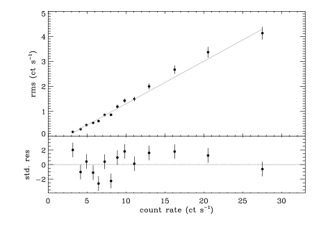
Figure 5: $0.2-10$ keV rms-flux relation. The rms is measured over the $1-10$ mHz range (see text for details). The solid line marks the best-fitting linear model. The lower panel shows the standardised residuals, i.e. (data – model)/error.

Figure 6: “Fluxed” EPIC pn spectra shown in $E\times F(E)$ units. Moving from top to bottom the spectra are: (1) from a bright flux interval (rev1730), (2) from a typical flux interval (rev1743) (3) from a faint interval (rev1739), (4) the offset of the rms-flux relation $C(E)$ (see text). Errors for the rms-flux offset spectrum are the errors on the linear regression parameter.

5 A search for quasi-periodic oscillations

The power spectral fitting discussed above provided no clear evidence for narrow features, i.e. QPOs. Such features are usually described in terms of Lorentzian “lines” seen in the power spectrum in addition to the continuum. In order to assess the evidence for a QPO more rigorously we defined two competing hypotheses: the null hypothesis $H_{0}$ of a continuum power spectrum, and the alternative hypothesis $H_{1}$ which includes an additional Lorentzian component.

$$H_{0}:P(\nu)=cont(\nu,\theta_{C})$$ (2)

$$H_{1}:P(\nu)=cont(\nu,\theta_{C})+qpo(\nu,\theta_{Q}).$$ (3)

where the continuum model is defined above (equation 1) and the QPO will be described by a Lorentzian profile

$$qpo(\nu,\theta_{Q})=\frac{2R^{2}Q\nu/\pi}{\nu_{\rm Q}^{2}+4(\nu-\nu_{\rm Q})^{2}}.$$ (4)

The parameters of the continuum are $\theta_{C}=\{\alpha_{\rm high},\nu_{\rm bend},N\}$ and the QPO parameters are $\theta_{Q}=\{\nu_{\rm Q},Q,R\}$, where $\nu_{\rm Q}$ is the centroid frequency, $Q$ is the width parameter ($Q=\nu_{\rm Q}/\Delta\nu$, where $\Delta\nu$ is the Full Width at Half Maximum), and $R$ is the amplitude parameter (equal to the total rms in the limit of high $Q$). See Pottschmidt et al. (2003) for details of this parameterisation. In the present case we have assumed two different values, namely $Q=5$ and $Q=10$, which are fairly typical values for high frequency QPOs in GBHs (e.g. Remillard et al., 2002, 2003). Using these two representative values rather than allowing $Q$ to be a free parameter made the QPO search and upper limit calculations (discussed later) much more efficient.

One of the simplest ways to select between these two competing models is to assess the improvement in the $\chi^{2}$ fit statistic upon the addition of the QPO, i.e. the difference between the minimum $\chi^{2}$ for $H_{0}$ and $H_{1}$. For a given dataset a large reduction (improvement) in the fit statistic between $H_{0}$ and $H_{1}$ is taken to be evidence in favour of a QPO. For the 2009 data, and the full $0.2-10$ keV energy band, the reduction in $\chi^{2}$ statistic was only $6.85$ (assuming $Q=10$, and a very similar value assuming $Q=5$), with best-fitting parameters $\nu_{Q}=3.8\pm 0.3$ mHz and $R=1.2\pm 0.5$ per cent. The modest improvement in the fit falls short of our threshold for a significant detection, as discussed below. The QPO search was repeated for the three energy bands discussed above, with very similar results. The $2$–$10$ keV band gave the largest improvement in the fit upon the addition of a QPO ($\Delta\chi^{2}=10.94$ assuming $Q=5$), but this still falls short of a detection in the $\alpha=0.01$ test.

The lack of detection may itself be an interesting result if the observation was sufficiently sensitive, and to assess this requires a calculation of the upper limit on the strength of a QPO. The first step is to define a precise detection procedure and then calibrate its statistical ‘power’ as a function of QPO strength. That would allow us to determine the weakest QPOs that would be detected with reasonable probability.

5.1 Detection procedure

The search for QPOs in binned power spectral data is no different from the search for “lines” in any other one dimensional spectrum, and suffers from the same statistical and computational challenges. See Freeman et al. (1999), Protassov et al. (2002), Park et al. (2008) for elaboration of the issues.

The difference in the minimum chi-square statistic for each model was used as a test statistic. For a dataset $\mathbf{x}$ we compute

$$T(\mathbf{x})=\chi^{2}(\mathbf{x},H_{0})-\chi^{2}(\mathbf{x},H_{1}).$$ (5)

The nuisance parameters – specifying the continuum and the QPO – are eliminated by minimisation, i.e. $\chi^{2}(\mathbf{x},H_{0})=\min_{\theta_{C}}[\chi^{2}(\mathbf{x},H_{0},\theta_{C})]$. This test statistic is closely related to the Likelihood Ratio Test (LRT), as has been discussed by Protassov et al. (2002). A large value of the test statistic (i.e. a large improvement in the fit upon adding a QPO to the model) is taken as evidence for a QPO.

The critical value of $T$ for detection, $T_{\rm crit}$, was calculated by a Monte Carlo method as discussed in Appendix B. In the present case we found $T_{\rm crit}=12.28$ for $\alpha=0.01$ (this is for $Q=10$, using $Q=5$ gave $13.05$ which is practically the same). In other words, assuming the continuum model to be true (with parameters represented by the posterior distribution $p(\theta_{C}\mid\mathbf{x}^{\rm obs})$ derived above from the real data), and no QPO, a reduction in the $\chi^{2}$ fit statistic of $T\geq 12.28$ will occur with probability $\alpha=0.01$ (and have a posterior predictive $p$-value $\leq 0.01$).

5.2 Upper limit procedure

In order to define an upper limit on the strength of possible QPOs we use the definition of an upper limit in terms of the power $\beta$ of a detection procedure, as discussed very clearly in the recent paper by Kashyap et al. (2010). A QPO of a given frequency and strength $(\nu_{Q},R)$ has a probability of detection $\beta(\nu_{Q},R)$ using the above method (for fixed $\alpha$).

We used a Monte Carlo method, as discussed in Appendix B, to estimate the detection probability $\beta(\nu_{Q},R)$ for a range of different QPO locations and strengths ($\nu_{Q}$ and $R$ values). The estimate is simply the fraction of simulations (for each $\nu_{Q}$ and $R$) that gave a significant detection defined by $T(\mathbf{x}^{\rm sim})\geq T_{\rm crit}$. Contours of constant $\beta$ on the $\nu_{Q}$-$R$ plane define the upper limit on the strength $R$ of a QPO as a function of frequency $\nu_{Q}$. Figure 7 shows the contours for $\beta=0.5$, $0.9$ and $>0.995$ assuming $Q=10$ (solid curves) and $Q=5$ (dotted curves). The middle of each set of curves represents the weakest QPO that could be present (at each frequency) and have a probability $\geq 0.9$ of being detected. This limit extends below $R=5$ per cent for $\nu\mathrel{\hbox{\hbox to0.0pt{\hbox{\lower 4.0pt\hbox{$\sim$}}\hss}\hbox{$>$}}}3\times 10^{-4}$ Hz, and below $R=2$ per cent for $\nu\mathrel{\hbox{\hbox to0.0pt{\hbox{\lower 4.0pt\hbox{$\sim$}}\hss}\hbox{$>$}}}3\times 10^{-3}$ Hz. The shape and amplitude of this curve is similar to that obtained using the simpler $\Delta\chi^{2}$ confidence contour method used previously by Vaughan & Uttley (2005).

Figure 7: Upper limit on the strength of a QPO, assumed to have a Lorentzian spectrum, defined for an $\alpha=0.01$ test. The solid curve was calculated assuming a $Q=10$ QPO and the dotted curve was calculated assuming $Q=5$. In each case the three curves show (from bottom to top) the upper limits corresponding $\beta=0.5,0.9$ and $>0.995$ powers. The detection power at each point in the plane was computed using $200$ Monte Carlo simulations of data with a QPO present and recording the fraction of simulations that gave a detection (using a $\Delta\chi^{2}\geq 12.28$ detection criterion for $Q=10$). See section 5 and Appendix B for details.

6 Long term stationarity

The power spectral estimation and fitting described in section 3 was repeated for the 2001 data. Figure 8 shows a comparison of the 2001 and 2009 power spectra which are in broad agreement in shape and overall (fractional) amplitude. The best-fitting bending power law model ($\chi^{2}=26.22$ for $27$ dof, $p=0.51$) had a slightly higher bend frequency ($\nu\approx 5.5\times 10^{-4}$ Hz with a $90$ per cent confidence interval of $[3.0,9.0]\times 10^{-4}$ Hz, and a credible interval of $[2.7,8.4]\times 10^{-4}$ Hz) and high-frequency index ($\alpha_{\rm high}=-2.48\pm 0.16$) compared to the 2009 data. The marginal distribution of $\nu_{\rm bend}$ from both datasets are shown in Fig 3. These appear to suggest there was a slight change in the power spectral shape between the two sets of observations. It is for this reason that we have not combined the 2001 and 2009 data to produce a composite power spectrum.

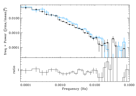
Figure 8: Comparison of 2009 and 2001 power spectrum estimates. Top panel: the estimated power spectra computed for the 2001 observation (blue histogram) and the combined 2009 observations (black; same as Figure 2). Bottom panel: ratio of the two estimates.

7 Discussion and conclusions

We have presented an analysis of the rapid X-ray flux variability of the low-mass Seyfert 1 galaxy NGC 4051 covering the range $10^{-4}$ to $\sim 2\times 10^{-2}$ Hz, based on a series of $15$ XMM-Newton observations taken during 2009. This is among the best X-ray power spectra for any active galaxy, and the large range of fluxes sampled during the observations has allowed for an examination of the flux-dependence of the variability. Below we discuss the results and, where possible, relate them to the known behaviour of GBHs (for which we use a fiducial mass of $M_{\rm BH}=10$ $\rm\thinspace M_{\odot}$).

7.1 Power spectral shape in relation to other sources

The power spectrum of the variations is well described by a bending power law model that bends from an index of $\alpha_{\rm low}\approx-1.1$ to $\alpha_{\rm high}\approx-2.3$ around $\nu_{\rm bend}\sim 2\times 10^{-4}$ Hz. This is fairly consistent with the M^cHardy et al. (2006) relation

$$\log(T_{\rm b})=2.1\log(M_{6})-0.98\log(L_{44})-2.32,$$ (6)

where $T_{\rm b}$ is the break timescale in days ($\nu_{\rm bend}=1.16\times 10^{-5}/T_{\rm b}$ Hz), $M_{\rm BH}=M_{6}10^{6}$ $\rm\thinspace M_{\odot}$, and $L_{\rm Bol}=L_{44}10^{44}$ erg s^-1 is the bolometric luminosity. The average $2-10$ keV X-ray flux during the 2009 observations was $F_{2-10}\approx 1.2\times 10^{-11}$ erg s^-1 cm^-2 which gives $L_{2-10}=3.5\times 10^{41}$ erg s^-1 at an assumed distance of $15.7$ Mpc (Russell, 2002), and $L_{\rm Bol}\sim 10^{43}$ (assuming a $L_{\rm Bol}/L_{2-10}\sim 27$; Elvis et al., 1994). The black hole mass is thought to be $M_{\rm BH}\sim 1.7\pm 0.5\times 10^{6}$ $\rm\thinspace M_{\odot}$(Denney et al., 2009), therefore $\dot{m}_{\rm Edd}\sim L_{\rm Bol}/L_{\rm Edd}\sim 0.05$. Together these give a predicted bend frequency of $8\times 10^{-5}$ Hz ($T_{\rm b}\sim 0.14$ day), within a factor $\sim 3$ of the observed value. In fact the estimated $\nu_{\rm bend}$ from the 2009 data is closer to the value expected from the M^cHardy et al. (2006) relation than that estimated by M^cHardy et al. (2004), when calculated using the revised black hole mass estimate (Denney et al., 2009, 2010).

The high frequency power spectrum above the bend rarely provides strong, unambiguous signatures of the accretion state of GBH systems, which tend to differ more at lower frequencies where features such as low frequency QPOs, flat-topped noise and broad Lorentzians occur (see e.g. van der Klis, 2006; McClintock & Remillard, 2006; Belloni, 2010). M^cHardy et al. (2004) suggested NGC 4051 may be analogous to a soft state (particularly like that seen in Cygnus X-1) on the basis of the low frequency noise (a $nu^{-1}$ spectrum extending over two decades or more), the high frequency slope ($\alpha_{\rm high}<-2$) and the value of $\nu_{\rm bend}$ (which tends to be higher in the soft state, making the ratio $T_{b}/M_{\rm BH}$ smaller).

For the 2009 data we found a very similar same high frequency shape and therefore is consistent with this identification. Ignoring any $\dot{m}$ dependence and simply scaling frequencies inversely with mass ($\nu_{\rm bend}\propto 1/M_{\rm BH}$), the bend frequency for NGC 4051 correponds to $\sim 34$ Hz in a typical GBH. This is close to the $\nu_{\rm bend}\approx 23$ Hz estimated from a soft state observation of Cygnus X-1 by M^cHardy et al. (2004).

The state analogy is supported by radio observations. At the highest available resolution the source is resolved into a core and two oppositely directed sources separated from the core by $\sim 0.4$ arcsec (Ulvestad & Wilson, 1984; Kukula et al., 1995; Ho & Ulvestad, 2001; Giroletti & Panessa, 2009). This structure is similar to the core and hotspots commonly seen in Fanaroff-Riley II radio galaxies, although no radio jet has been detected in NGC 4051. Jones et al. (2010) recently used radio monitoring observations and found no evidence for strong variability of the core flux. Despite the presence of these radio sources, Jones et al. (2010) showed that NGC 4051 falls below the ‘fundamental plane’ connecting the radio and X-ray luminosities to black hole mass in radio loud AGN and hard-state GBHs (Merloni et al., 2003; Falcke et al., 2004; Körding et al., 2006), i.e. it is less radio-loud than would be expected for a hard-state or radio-loud system (see Fig. 14 of Jones et al., 2010). This is consistent with the ‘soft state’ interpretation of NGC 4051 mentioned above.

The XMM-Newton data reveal the power spectrum of NGC 4051 up to frequencies as high as $\mathrel{\hbox{\hbox to0.0pt{\hbox{\lower 4.0pt\hbox{$\sim$}}\hss}\hbox{$>$}}}10^{-2}$ Hz (see Fig 2 and 4), a factor $\sim 40$ above the bend frequency $\nu_{\rm bend}$. Assuming a black hole mass as above, the gravitational radius is $r_{g}=GM/c^{2}\approx 2.5\times 10^{6}$ km, and the period of the innermost stable circular orbit (ISCO) should be $\sim 100-800$ s, depending on the dimensionless spin parameter, $j$ (see e.g. van der Klis, 2006, and references therein). The power spectrum of NGC 4051 above $\nu_{\rm bend}$ shows no indication of deviating from a power law up to the highest frequencies (but see section 7.3), and in particular shows no signature of the ISCO period, which might be expected to produce an excess of variability power due to Doppler boosting of “hot spots” (Revnivtsev et al., 2000; Syunyaev, 1973). There is no sign of the additional power spectral break seen at very high frequencies in the hard state of Cygnus X-1 by Revnivtsev et al. (2000). Indeed, assuming linear scaling of timescales with black hole mass, we detect power at frequencies corresponding to $\sim 1.7$ kHz for a GBH, far above the fastest variations yet detected from these sources (Revnivtsev et al., 2000; Strohmayer, 2001).

7.2 Stationarity and the existence of “states”

The location of the power spectrum bend frequency is lower than that reported by M^cHardy et al. (2004) from their analysis of the 2001 XMM-Newton data. The $90$ per cent confidence intervals from these two analyses – $[5,12]\times 10^{-4}$ mHz and $[1.4,3.3]\times 10^{-4}$ Hz – do not overlap, although some of this may be due to the interval reported by M^cHardy et al. (2004) being an underestimate (see Mueller & Madejski, 2009). The difference between the two results may in part be due to differences in the data reduction and power spectrum estimation techniques; the re-analysis of the 2001 data presented here (section 6) gives a lower $\nu_{\rm bend}$ estimate and shows the difference between the two observations to be only moderately statistically significant (compare also the Bayesian posterior distributions of Fig 3). If this is a real effect, it is different from the expected scaling of $\nu_{\rm bend}$ with accretion rate in the central region implied by the M^cHardy et al. (2006) relation, since the X-ray luminosity in the month leading up to the 2009 observation (based on the RXTE monitoring) was $\sim 20$ per cent higher than in the month leading up to the 2001 observations, but the bend frequency was $\sim 60$ per cent lower.

The separation of $\sim 8$ years between the two observations corresponds to a separation of only $\sim 30$ minutes for a $10$ $\rm\thinspace M_{\odot}$GBH; on these timescales GBH power spectra are approximately stationary except during very rapid state transitions. By the same linear scaling each of the $\sim 40$ ks XMM-Newton observations is equivalent to $\sim 0.2$ s, and the $45$ day span of the observations covers the equivalent of only $\sim 20$ s for a typical GBH. Unless NGC 4051 is drastically more non-stationary that most GBHs we might therefore expect all the XMM-Newton observations to be representative of almost exactly the same state and variability properties.

During both the 2001 and 2009 observations the variability does, to a very good approximation, follow a single rms-flux relation over the full flux range (see Figure 5) and the shape of the power spectrum remains roughly the same at different flux levels (see Figure 4). The lack of variability during low flux intervals (e.g. rev1739) and the extreme variability during high flux intervals (rev1730) are opposite extremes of this relation. These apparently different behaviours are therefore not the result of distinct variability states, despite their very different energy spectra (see Figure 6). (See also Uttley et al. 2003.) The variations in energy spectral shape are also continuous, as discussed by Vaughan et al. (2010, in prep.).

7.3 Absence of QPOs

We found no strong evidence (using a $\alpha=0.01$ test) for QPOs (additional, narrow components) in the 2009 power spectrum, and we place limits of $R\mathrel{\hbox{\hbox to0.0pt{\hbox{\lower 4.0pt\hbox{$\sim$}}\hss}\hbox{$<$}}}2$ per cent rms on the strength of a QPO in the $\mathrel{\hbox{\hbox to0.0pt{\hbox{\lower 4.0pt\hbox{$\sim$}}\hss}\hbox{$>$}}}3\times 10^{-3}$ Hz range, and $\mathrel{\hbox{\hbox to0.0pt{\hbox{\lower 4.0pt\hbox{$\sim$}}\hss}\hbox{$<$}}}5-10$ per cent over the $10^{-4}-3\times 10^{-3}$ Hz range. The $10^{-3}-0.1$ Hz bandpass over which these data are sensitive to weak QPOs corresponds to $\mathrel{\hbox{\hbox to0.0pt{\hbox{\lower 4.0pt\hbox{$\sim$}}\hss}\hbox{$>$}}}170$ Hz for a GBH, where HF QPOs are often found, and the upper limit of $R\sim 2$ per cent on the QPO strength is comparable to the strength of typical HF QPOs (Remillard et al., 2003). Such HF QPOs been detected in GBHs only in intermediate states (particularly the soft intermediate state; Belloni, 2010), but are not always present (at least not at detectable levels), and when detected may be strongly energy-dependent. The lack of detection in NGC 4051 therefore does not constitute strong evidence against an analogous state in this AGN.

Despite not being formally significant in an $\alpha=0.01$ test, the best-fitting narrow Lorentzian QPO component has a frequency of $\nu_{Q}=4\times 10^{-3}$ Hz and rms $R\sim 1$ per cent. This frequency is very close to that found previously by Vaughan & Uttley (2005) from fitting the power spectrum of the 2001 data. This may be a coincidence in the random sampling fluctuations around a smooth continuum power spectrum. But it is around this frequency that the signal-to-noise in the data is highest, and so model fitting will be most sensitive to small ($\sim 20$ per cent) deviations from the smooth power law model. The high frequency power law may be only an approximation to a more complex continuum power spectrum, the structure of which is on the edge of detectability in these data.

It is well known that HF QPOs in GBHs can be strongly energy dependent, and frequently stronger at higher energies, and in fact we did find the higher energy band ($2$–$10$ keV) gave slightly stronger evidence for a possible QPO. But this could also indicate that this energy band contains a stronger contribution from a second, variable emission component with a different power spectrum from that which dominates the softer energy bands.

7.4 A quasi-constant emission component

The flux offsets in the energy-resolved rms-flux relations, $C(E)$, reveals the spectrum of a quasi-constant component (QC) of the emission. A simple model comprising a single power law ($\Gamma=3.06\pm 0.13$) modified by Galactic absorption (Elvis et al., 1989) gave a very good fit, with $\chi^{2}=10.65$ for $18$ dof. A Comptonising plasma model (compTT) with optical depth $\tau=1$ and seed photon energy $\sim 50$ eV, which has an approximately power law shape, also gave a good fit ($\chi^{2}=9.45$ for $17$ dof). The simplest interpretation is that this represents an emission component that does not vary at all during the 2009 observations; emission that remains if the highly variable emission component(s) drop to zero flux. We note that the Chandra data taken during an extended low flux period in 2001 and the XMM-Newton observation taken during a low flux period in 2002 were previously interpreted in terms of an unresolved ($\mathrel{\hbox{\hbox to0.0pt{\hbox{\lower 4.0pt\hbox{$\sim$}}\hss}\hbox{$<$}}}100$ pc), non-varying soft spectral component and a strongly variable, harder spectral component (Uttley et al., 2003, 2004). However, the QC emission is not required to be absolutely constant over the observations, it is only required to have a far lower (absolute) amplitude (at $\mathrel{\hbox{\hbox to0.0pt{\hbox{\lower 4.0pt\hbox{$\sim$}}\hss}\hbox{$>$}}}1$ mHz) and be weakly correlated (or uncorrelated) with the highly variable component that dominates brighter flux spectra (e.g. rev1730) and drives the rms-flux relation.

The spectral shape and absolute flux level of this component are similar to the lowest flux spectrum taken during 2009 (rev1739) below $\sim 2$ keV, as shown in Figure 6. This strongly suggests that most of the soft X-ray continuum emission observed during low flux periods is due to the soft QC component. This may be the tail of the spectrum of inverse-Compton scattering of optical-UV continuum photons in shock-heated gas where the ionised outflow collides with the inter-stellar medium of the host galaxy, as recently predicted to occur in AGN by King (2010). Indeed, the velocity-ionisation structure of the outflow as resolved by the RGS data provide further evidence to support this scenario (Pounds & Vaughan, 2011).

Appendix A Construction of ‘fluxed’ spectra

X-ray spectra are conventionally given in terms of count rates per detector channel. These “raw” spectra are of limited use for data visualisation because of the distorting effect of (i) the energy-dependent efficiency of the telescope and detector (described by the effective area function), and (ii) blurring by the line spread function of the instrument (modelled by the redistribution matrix). The true source spectrum $S(E)$ (in units of photon s^-1 cm^-2 keV^-1) is related to the observed count rate in channel $i$ by a Fredholm integral equation:

$$C(i)=\int R(i,E)A(E)S(E)dE$$ (7)

where $A(E)$ is the instrument effective area (cm²) and $R(i,E)$ gives the probability that a photon of energy $E$ will be recorded in channel $i$ (i.e. the redistribution function). Here the observed spectrum $C(i)$ is assumed to be background-subtracted, and the instrumental response defined by $R(i,E)A(E)$ is assumed to be linear, that is, independent of the value of $S(E)$ which is a good approximation so long as pile-up is negligible. This integral equation can be approximated using a discrete formulation in which the energy range is divided into $N$ bins $E_{j}$:

$$C_{i}=\sum_{j=1}^{N}R_{ij}A_{j}S_{j}$$ (8)

where $R_{ij}$ is the average and $A_{j}$ and $S_{j}$ are the definite integrals of their continuous counterparts, over the energy range of each bin $E_{j}\rightarrow E_{j+1}$.

In general, methods that attempt to invert the above equations to recover $S(E)$ from an observed spectrum $C_{i}$ are unreliable and one must turn to the ‘forward fitting’ method to build a model of the spectrum (see Arnaud, 1996). However, it is often useful to view even an approximate ‘fluxed’ spectrum, largely free from the distorting effects of the instrument efficiency, if only to give a better visual representation of the underlying source spectrum. Nowak (2005) discussed a simple method to accomplish this in which the observed count spectrum is normalised by an effective area curve that has been blurred using the redistribution function.

$$\hat{S}_{i}=C_{i}/\sum_{j=1}^{N}R_{ij}A_{j}$$ (9)

This method matches the blurring of the effective area to the blurring of the observed spectrum to give an estimate of the spectrum in true flux units (e.g. photon s^-1 cm^-2) that is, to a large extent, free from the distorting effects of the energy-dependent effective area. This process is essentially equivalent to calibrating the sensitivity using an observation of an ideal standard star (with a perfectly flat spectrum). The resulting spectrum can easily be converted to conventional flux density units (e.g. erg s^-1 cm^-2 keV^-1).

It is crucial that the effective area function $A_{j}$ is blurred by the redistribution matrix. The reason is that the effective area function may contain abrupt changes in efficiency (e.g. near photoelectric edges in the detector-mirror system, such as the K-edges of O and Si, or the M-edge of Au) that can be far sharper than the resolving power of the detector, which means that normalising the observed (blurred) spectrum by the exact (not blurred) effective area introduces very strong spurious features into the spectrum near the edges. Blurring the effective area curve matches the resolution to that of the data and suppresses this effect. The result is a spectrum with the energy-dependence of the detector/mirror efficiency removed (to a reasonable approximation), but which remains at the detector spectral resolution. We emphasise that this is not, even approximately, a deconvolved spectrum. It has the advantage over the popular ‘unfolding’ method (in XSPEC) of being independent of the spectral model, and therefore providing a more objective visualisation ‘fluxed’ spectrum.

Appendix B QPO detection and upper limits

This appendix presents first an outline of the method used to search for QPOs in the power spectral data, and second how upper limits were derived based on the detection method.

B.1 Calibrating the QPO detection procedure

An $\alpha$-threshold detection procedure uses a test statistic $T$ to quantify evidence for a detection, and is calibrated such that a detection occurs when $T(\mathbf{x})>T_{\rm crit}$ for some threshold value $T_{\rm crit}$ chosen to have a small probability $\alpha$ of occurring by chance when $H_{0}$ is true. Specifically, the detection threshold is chosen such that $\Pr(T>T_{\rm crit}\mid H_{0})\leq\alpha$, where $\alpha$ is the chance of a ‘false detection’ (a ‘type I error’ when $H_{0}$ is true). Commonly used values are $\alpha=0.05$ and $0.01$. But in order to calculate $T_{\rm crit}$ we need to know the reference distribution of the test statistic on the assumption that the null hypothesis is true, $p(T\mid H_{0})$. In general this may be estimated by calculating the distribution of the test statistic from a large number of Monte Carlo simulations of data generated assuming $H_{0}$ and distributed as expected for realistic data.

The above would be valid if the null hypothesis was simple, that is, did not contain any unknown (free) parameters. In the present case the null hypothesis does involve parameters estimated using the observed data, $\theta_{C}$. We account for the uncertainties in their values by using random parameters drawn from the posterior distribution to generate the simulated data, using the MCMC discussed in section 3. This gives the distribution of the test statistic known as the posterior predictive distribution (see Rubin, 1984; Meng, 1994; Gelman et al., 1996, 2004; Protassov et al., 2002; Vaughan, 2010).

$$p(T\mid H_{0},\mathbf{x}^{\rm obs})=\int p(T\mid H_{0},\theta_{C})p(\theta_{C}|\mathbf{x}^{\rm obs})d\theta_{C}$$ (10)

In order to determine $T_{\rm crit}$ this distribution was mapped out using Monte Carlo simulations as follows:

• repeat for $k=1,2,...,N$ simulated datasets:

  1. Draw a set of parameter values from the posterior $\theta_{C}^{k}$

  2. simulate data from $H_{0}$ with parameters $\theta_{C}^{k}$: $\mathbf{x}^{k}$

  3. fit $H_{0}$ to get $\chi^{2}(\mathbf{x}^{k},H_{0})$

  4. fit $H_{1}$ to get $\chi^{2}(\mathbf{x}^{k},H_{1})$

  5. compute $T^{k}$

• use the distribution of $T^{k}$ to define $T_{\rm crit}$ for which $\Pr(T>T_{\rm crit}\mid H_{0})\leq\alpha$

We used $N=3,000$ simulations to calibrate $T_{\rm crit}$ and found the critical value for an $\alpha=0.01$ test was $T_{\rm crit}=12.28$. (This was calculated using a $Q=10$ QPO, but using $Q=5$ gave a very similar result.) for the data and models discussed in this paper. In order to ensure the global minimum was found in each case (this can be tricky for $H_{1}$ which may produce multiple minima in $\chi^{2}$) we used the robust automated fitting scheme discussed by Hurkett et al. (2008, section 3.2.2)

B.2 Upper limit procedure

We wish to determine the upper limit $U$ on the QPO strength $R$, which is the smallest value of $R$ such the probability of detecting the QPO (assuming it is present, i.e. $H_{1}$) is $\geq\beta_{\rm min}$ for some specific $\beta_{\rm min}$. See Kashyap et al. (2010) for a very clear introduction to the meaning and calculation of upper limits in astronomy.

In the present case we are searching for a QPO of unknown location (frequency) but the upper limit may vary as a function of this location – because the “background” continuum level and the uncertainty on the spectrum vary as a function of frequency – so we must calculate the limit for a set of different QPO locations $\nu_{Q}$. The probability of a detection, $\beta$, which is $1-$(probability of ‘type II error’), is:

$$\beta(\nu_{Q},R)=\Pr(T\geq T_{\rm crit}\mid H_{1},\nu_{Q},R)$$ (11)

and the upper limit $U(\nu_{Q})$ is the smallest value of $R$ which satisfies

$$\beta(\nu_{Q},R)\geq\beta_{\rm min}$$ (12)

for some chosen minimum power $\beta_{\rm min}$.

Given the $T_{\rm crit}$ defined above we can compute the upper limit using Monte Carlo simulations of realistic data under $H_{1}$. These can be used to map out the distribution $p(T\mid H_{1},\nu_{Q},R)$ for different $\nu_{Q}$ and $R$ values, and hence find $U(\nu_{Q})$ that satisfies the above equations. In these terms the upper limit is the strength of the weakest QPO that would have a reasonable probability $\beta\geq\beta_{\rm min}$, for some specific $\beta_{\rm min}$ such as $0.5$ or $0.9$.

This method will, in general, be sensitive to the parameters of the continuum model, $\theta_{C}$, which of course we do not know exactly. But, as before, we can average over the posterior distribution of these as derived from the data $p(\theta_{C}\mid\mathbf{x}^{\rm obs})$.

$$p(T\mid H_{1},\nu_{Q},R)=\int p(T\mid H_{1},\nu_{Q},R,\theta_{C})p(\theta_{C}\mid\mathbf{x}^{\rm obs})d\theta_{C}.$$ (13)

Again, this can be done be tacking values from the posterior using the MCMC discussed in section 3.

The calculation of $\beta$ for a given pair of QPO parameters ($\nu_{Q}$ and $R$) was performed using a Monte Carlo scheme as follows.

• loop over $k=1,2,...,N$ simulated datasets

  1. Draw a set of parameter values from the posterior $\theta_{C}^{k}$

  2. simulate data from $H_{1}$ with continuum parameters $\theta_{C}^{k}$ and QPO parameters ($\nu_{Q},R$): $\mathbf{x}^{k}$

  3. fit $H_{0}$ to get $\chi^{2}(\mathbf{x}^{k},H_{0})$

  4. fit $H_{1}$ to get $\chi^{2}(\mathbf{x}^{k},H_{1})$

  5. compute $T_{k}$

• use distribution of $T^{k}$ to find $\beta(\nu_{Q},R)=\Pr(T>T_{\rm crit}\mid H_{1},\nu_{Q},R)$

This process is repeated over a grid of QPO parameters, $\nu_{Q}$ and $R$, and at each frequency $\nu_{Q}$ the smallest $R$ for which $\beta(\nu_{Q},R)\geq\beta_{\rm min}$ is the upper limit $U(\nu_{Q})$. For the present analysis we used $30$ logarithmically spaced values of QPO location $\nu_{Q}$, $40$ logarithmically spaced values of QPO strength $R$, and at each pair generated $N=200$ simulations. This is a sufficient number of simulations to accurately define contours of e.g. $\beta=0.9$ on the $\nu_{Q}$-$R$ plane.

The detection procedure was calibrated using simulated data generated assuming $H_{0}$. But to evaluate $\beta$, and hence the upper limit, the data were simulated assuming $H_{1}$. The former is concerned with the chance of spurious detection assuming no QPO present, the latter is concerned with the chance of detection when a QPO is present.

References

- Arévalo et al. (2008) Arévalo P., McHardy I. M., Summons D. P., 2008, MNRAS, 388, 211
- Arnaud (1996) Arnaud K. A., 1996, in G. H. Jacoby & J. Barnes ed., Astronomical Data Analysis Software and Systems V Vol. 101 of Astronomical Society of the Pacific Conference Series, XSPEC: The First Ten Years. p. 17
- Belloni (2010) Belloni T. M., 2010, in T. Belloni ed., Lecture Notes in Physics, Berlin Springer Verlag Vol. 794 of Lecture Notes in Physics, Berlin Springer Verlag, States and Transitions in Black Hole Binaries. p. 53
- Collinge et al. (2001) Collinge M. J., Brandt W. N., Kaspi S., Crenshaw D. M., Elvis M., Kraemer S. B., Reynolds C. S., Sambruna R. M., Wills B. J., 2001, ApJ, 557, 2
- Denney et al. (2010) Denney K. D., Peterson B. M., Pogge R. W., Adair A., Atlee D. W., Au-Yong K., Bentz M. C., Bird J. C., et al. 2010, ApJ, 721, 715
- Denney et al. (2009) Denney K. D., Watson L. C., Peterson B. M., Pogge R. W., Atlee D. W., Bentz M. C., Bird J. C., Brokofsky D. J., et al. 2009, ApJ, 702, 1353
- Done & Gierliński (2005) Done C., Gierliński M., 2005, MNRAS, 364, 208
- Edelson & Nandra (1999) Edelson R., Nandra K., 1999, ApJ, 514, 682
- Elvis et al. (1989) Elvis M., Wilkes B. J., Lockman F. J., 1989, AJ, 97, 777
- Elvis et al. (1994) Elvis M., Wilkes B. J., McDowell J. C., Green R. F., Bechtold J., Willner S. P., Oey M. S., Polomski E., Cutri R., 1994, ApJS, 95, 1
- Fabian (1979) Fabian A. C., 1979, Royal Society of London Proceedings Series A, 366, 449
- Falcke et al. (2004) Falcke H., Körding E., Markoff S., 2004, A&A, 414, 895
- Fender et al. (2004) Fender R. P., Belloni T. M., Gallo E., 2004, MNRAS, 355, 1105
- Fender et al. (2006) Fender R. P., Körding E., Belloni T., Uttley P., McHardy I., Tzioumis T., 2006 Vi microquasar workshop: Microquasars and beyond. Proceedings of Science: SISSA, Trieste (Italy), (arXiv:0706.3838)
- Freeman et al. (1999) Freeman P. E., Graziani C., Lamb D. Q., Loredo T. J., Fenimore E. E., Murakami T., Yoshida A., 1999, ApJ, 524, 753
- Gaskell (2004) Gaskell C. M., 2004, ApJL, 612, L21
- Gelman et al. (2004) Gelman A., Carlin J. B., Stern H. S., B. R. D., 2004, Bayesian Data Analysis (2nd ed). Chapman & Hall, London
- Gelman et al. (1996) Gelman A., Meng X.-L., Stern H. S., 1996, Statistica Sinica, 6, 733
- Gelman & Rubin (1992) Gelman A., Rubin D. B., 1992, Statistical Science, 7, 457
- Gierliński et al. (2008) Gierliński M., Middleton M., Ward M., Done C., 2008, Nature, 455, 369
- Gierliński et al. (2008) Gierliński M., Nikołajuk M., Czerny B., 2008, MNRAS, 383, 741
- Giroletti & Panessa (2009) Giroletti M., Panessa F., 2009, ApJL, 706, L260
- Gleissner et al. (2004) Gleissner T., Wilms J., Pottschmidt K., Uttley P., Nowak M. A., Staubert R., 2004, A&A, 414, 1091
- Hayashida et al. (1998) Hayashida K., Miyamoto S., Kitamoto S., Negoro H., Inoue H., 1998, ApJ, 500, 642
- Heinz & Sunyaev (2003) Heinz S., Sunyaev R. A., 2003, MNRAS, 343, L59
- Ho & Ulvestad (2001) Ho L. C., Ulvestad J. S., 2001, ApJS, 133, 77
- Hurkett et al. (2008) Hurkett C. P., Vaughan S., Osborne J. P., O’Brien P. T., Page K. L., Beardmore A., Godet O., Burrows D. N., Capalbi M., Evans P., Gehrels N., Goad M. R., Hill J. E., Kennea J., Mineo T., Perri M., Starling R., 2008, ApJ, 679, 587
- Jones et al. (2010) Jones S., McHardy I., Moss D., Seymour N., Breedt E., Uttley P., Kording E., Tudose V., 2010, ArXiv e-prints
- Kashyap et al. (2010) Kashyap V. L., van Dyk D. A., Connors A., Freeman P. E., Siemiginowska A., Xu J., Zezas A., 2010, ApJ, 719, 900
- King (2010) King A. R., 2010, MNRAS, 402, 1516
- Körding et al. (2006) Körding E. G., Jester S., Fender R., 2006, MNRAS, 372, 1366
- Kukula et al. (1995) Kukula M. J., Pedlar A., Baum S. A., O’Dea C. P., 1995, MNRAS, 276, 1262
- Lawrence et al. (1987) Lawrence A., Watson M. G., Pounds K. A., Elvis M., 1987, Nature, 325, 694
- Markowitz et al. (2003) Markowitz A., Edelson R., Vaughan S., Uttley P., George I. M., Griffiths R. E., Kaspi S., Lawrence A., McHardy I., Nandra K., Pounds K., Reeves J., Schurch N., Warwick R., 2003, ApJ, 593, 96
- McClintock & Remillard (2006) McClintock J. E., Remillard R. A., 2006, in Lewin, W. H. G. & van der Klis, M. ed., Compact stellar X-ray sources Black hole binaries. pp 157–213
- McHardy et al. (2007) McHardy I. M., Arévalo P., Uttley P., Papadakis I. E., Summons D. P., Brinkmann W., Page M. J., 2007, MNRAS, 382, 985
- McHardy et al. (2006) McHardy I. M., Koerding E., Knigge C., Uttley P., Fender R. P., 2006, Nature, 444, 730
- McHardy et al. (2004) McHardy I. M., Papadakis I. E., Uttley P., Page M. J., Mason K. O., 2004, MNRAS, 348, 783
- Meng (1994) Meng X.-L., 1994, Annals of Statistics, 22, 1142
- Merloni et al. (2003) Merloni A., Heinz S., di Matteo T., 2003, MNRAS, 345, 1057
- Middleton & Done (2010) Middleton M., Done C., 2010, MNRAS, 403, 9
- Middleton et al. (2009) Middleton M., Done C., Ward M., Gierliński M., Schurch N., 2009, MNRAS, 394, 250
- Miyamoto et al. (1991) Miyamoto S., Kimura K., Kitamoto S., Dotani T., Ebisawa K., 1991, ApJ, 383, 784
- Mueller & Madejski (2009) Mueller M., Madejski G., 2009, ApJ, 700, 243
- Mushotzky et al. (1993) Mushotzky R. F., Done C., Pounds K. A., 1993, Ann. Rev. A&A, 31, 717
- Nandra & Papadakis (2001) Nandra K., Papadakis I. E., 2001, ApJ, 554, 710
- Nowak (2005) Nowak M., 2005, Ap&SS, 300, 159
- Ogle et al. (2004) Ogle P. M., Mason K. O., Page M. J., Salvi N. J., Cordova F. A., McHardy I. M., Priedhorsky W. C., 2004, ApJ, 606, 151
- Papadakis & Lawrence (1993) Papadakis I. E., Lawrence A., 1993, MNRAS, 261, 612
- Papadakis & Lawrence (1995) Papadakis I. E., Lawrence A., 1995, MNRAS, 272, 161
- Park et al. (2008) Park T., van Dyk D. A., Siemiginowska A., 2008, ApJ, 688, 807
- Ponti et al. (2006) Ponti G., Miniutti G., Cappi M., Maraschi L., Fabian A. C., Iwasawa K., 2006, MNRAS, 368, 903
- Pottschmidt et al. (2003) Pottschmidt K., Wilms J., Nowak M. A., Pooley G. G., Gleissner T., Heindl W. A., Smith D. M., Remillard R., Staubert R., 2003, A&A, 407, 1039
- Pounds et al. (2004) Pounds K. A., Reeves J. N., King A. R., Page K. L., 2004, MNRAS, 350, 10
- Pounds & Vaughan (2011) Pounds K. A., Vaughan S., 2011, MNRAS, in press, arXiv:1012.0998
- Protassov et al. (2002) Protassov R., van Dyk D. A., Connors A., Kashyap V. L., Siemiginowska A., 2002, ApJ, 571, 545
- Remillard et al. (2003) Remillard R., Muno M., McClintock J. E., Orosz J., 2003, in P. Durouchoux, Y. Fuchs, & J. Rodriguez ed., New Views on Microquasars X-ray QPOs in black-hole binary systems. p. 57
- Remillard & McClintock (2006) Remillard R. A., McClintock J. E., 2006, Ann. Rev. A&A, 44, 49
- Remillard et al. (1999) Remillard R. A., Morgan E. H., McClintock J. E., Bailyn C. D., Orosz J. A., 1999, ApJ, 522, 397
- Remillard et al. (2002) Remillard R. A., Muno M. P., McClintock J. E., Orosz J. A., 2002, ApJ, 580, 1030
- Revnivtsev et al. (2000) Revnivtsev M., Gilfanov M., Churazov E., 2000, A&A, 363, 1013
- Rubin (1984) Rubin D. B., 1984, Annals of Statistics, 12, 1151
- Russell (2002) Russell D. G., 2002, ApJ, 565, 681
- Shakura & Sunyaev (1976) Shakura N. I., Sunyaev R. A., 1976, MNRAS, 175, 613
- Steenbrugge et al. (2009) Steenbrugge K. C., Fenovčík M., Kaastra J. S., Costantini E., Verbunt F., 2009, A&A, 496, 107
- Strohmayer (2001) Strohmayer T. E., 2001, ApJL, 552, L49
- Syunyaev (1973) Syunyaev R. A., 1973, SvA J, 16, 941
- Terashima et al. (2009) Terashima Y., Gallo L. C., Inoue H., Markowitz A. G., Reeves J. N., Anabuki N., Fabian A. C., Griffiths R. E., Hayashida K., Itoh T., Kokubun N., Kubota A., Miniutti G., Takahashi T., Yamauchi M., Yonetoku D., 2009, PASJ, 61, 299
- Tomsick et al. (2004) Tomsick J. A., Kalemci E., Kaaret P., 2004, ApJ, 601, 439
- Ulvestad & Wilson (1984) Ulvestad J. S., Wilson A. S., 1984, ApJ, 285, 439
- Uttley et al. (2003) Uttley P., Fruscione A., McHardy I., Lamer G., 2003, ApJ, 595, 656
- Uttley & McHardy (2001) Uttley P., McHardy I. M., 2001, MNRAS, 323, L26
- Uttley et al. (2002) Uttley P., McHardy I. M., Papadakis I. E., 2002, MNRAS, 332, 231
- Uttley et al. (2005) Uttley P., McHardy I. M., Vaughan S., 2005, MNRAS, 359, 345
- Uttley et al. (2004) Uttley P., Taylor R. D., McHardy I. M., Page M. J., Mason K. O., Lamer G., Fruscione A., 2004, MNRAS, 347, 1345
- van der Klis (1989) van der Klis M., 1989, in Ögelman H., van den Heuvel E. P. J., eds, Timing Neutron Stars . p. 27
- van der Klis (1997) van der Klis M., 1997, in G. J. Babu & E. D. Feigelson ed., Statistical Challenges in Modern Astronomy II Quantifying Rapid Variability in Accreting Compact Objects. p. 321
- van der Klis (2006) van der Klis M., 2006, in Lewin, W. H. G. & van der Klis, M. ed., Compact stellar X-ray sources Rapid X-ray Variability. pp 39–112
- Vaughan (2010) Vaughan S., 2010, MNRAS, 402, 307
- Vaughan et al. (2003) Vaughan S., Edelson R., Warwick R. S., Uttley P., 2003, MNRAS, 345, 1271
- Vaughan & Fabian (2003) Vaughan S., Fabian A. C., 2003, MNRAS, 341, 496
- Vaughan et al. (2003) Vaughan S., Fabian A. C., Nandra K., 2003, MNRAS, 339, 1237
- Vaughan & Uttley (2005) Vaughan S., Uttley P., 2005, MNRAS, 362, 235
- Vaughan & Uttley (2006) Vaughan S., Uttley P., 2006, Advances in Space Research, 38, 1405